Risk aversion and expected-utility theory A calibration theorem
行为金融学的理论框架

行为金融学的理论框架行为金融学的理论框架 200607自1980年代以来,行为金融学逐渐受到重视,此研究领域相关理论的起源有二:一方面是因为许多实证研究发现传统理论无法解释的异常现象;另一方面则是和Kahneman and Tverskey(1979,以下简称为KT)所发表的展望理论有关。
本文试图针对展望理论与其他相关理论作详尽的介绍。
文章的这一部分只是作者预期的最后成稿的一个基础,希望在接下来的一段时间之内给出展望理论的相关研究结果,和行为金融学的其他理论发展。
一、展望理论(一)理论发展KT(1979)指出传统预期效用理论无法完全描述个人在不确定情况下的决策行为。
他们以大学教授和学生为基础进行问卷调查,发现大部分受访者的回答显示许多偏好违反传统预期效用理论的现象,并据此提出另一种经济行为的模型,称为展望理论。
KT将这些违反传统预期效用理论的部分归纳出下列三个效应来说明:⑴确定性效应(certainty effect)此效应是指相对与不确定的结局(outcome)来说,个人对于结果确定的结局会过度重视。
KT设计了两个问题来说明确定效应。
第一个问题是,假设有两个赌局:第一个赌局有33%的机会得到2,500元,66%的机会得到2,400元,另外1%的机会什么也没有,第二个督军是确定得到2,400,问卷的结果显示有82%的受访者选择第二个赌局。
第二个问题也假设有两个赌局:第一个赌局有33%的机会得到2,500元,67%的机会什么也没有。
第二个赌局有34%的机会得到2,400元,66%的机会什么也没有。
问卷的结果显示有83%的受访者选择第一个赌局。
比较以上两个问题可知,根据预期效用理论,第一个问题的偏好为?u(2,400)>0.33u(2,500)+0.66u(2,400)或0.34u(2,400)>0.33u(2,500),其中u(.)为效用函数。
第二个问题的偏好却是0.34u(2,400)<u(2,500),这明显地违反预期效用理论。
第六章风险厌恶与风险资产的配置

风险、投机与赌博
投机:为获得相应的报酬而承担一定的商业风险。
注意: 1、明确“相应的报酬”和“一定的风险”含义。 “相应的报酬”是指除去无风险收益之后的实际期望收益,它 或者是超额收益或者是风险溢价。--比如,投资者如果选择股 票,他希望获得的是股票期望收益高于国库券期望收益的风险 溢价。 “一定的风险”是指足以影响决策的风险,当增加的收益不足 以补偿所冒的风险时,投资者会放弃产生正的风险溢价的机会。
U1
U2
B X
A
3、同一个投资者有无限多条无差异曲线
对任何一个风险收益组合,投资者对其的偏好程度都
能与其他组合相比。无差异曲线图中越靠左上方的无差异
曲线代表的满足程度越高,投资者的目标尽力选择在左上角。
4、同一投资者在同一时间、同一时点的任何两条无差异
曲线都不能相交
假设某个投资者的两条无差异曲线相交于X点。由于X和
2、风险厌恶。现代投资组合理论还假设,投资者是 风险厌恶的,即在其他条件相同的情况下,投资者将 选择标准差较小的组合。
3
本章主要内容
投资者的风险态度 投资组合的效用评分方法 单一风险资产与单一无风险资产的投资
组合 资本配置线(CAL) 最优资本配置比例 资本市场线(CML)
4
6.1 风险与风险厌恶
率存在一定的低估 习惯以货币市场基金作为对绝大部分投资者
易接受的无风险资产
– 无风险利率有时可用LIBOR(伦敦银行同业拆放 利率 )来代替
28
6.4 单一风险资产与单一无风险资产的资产组合
记风险资产组合P的期望收益率为E
(rP
),
标准差为
,
P
无风险资产组合F的收益率为rf ,
CCPAM-1

• We have:
f
E (e ) = e
X
c −γ ln t+1 ct −1
E ( X ) + 0.5σ 2
1 1 −γ Et (∆ln ct+1 )+0.5γ 2σ 2 (∆ln ct+1 ) −1 R = Et (e ) = e β β r f = δ + γ Et (∆ ln ct +1) − 0.5γ 2σ 2 (∆ ln ct +1) where : r f = ln R f ; β = e−δ , ∆ ln ct +1 = ln ct +1 − ln ct
pt u′(ct +1 ) xt +1 = Et [ β ] Πt u ′(ct ) Π t +1
• Obviously, it is the same as defining a nominal discount factor by
u ′(ct +1 ) Π t pt = Et [( β ) xt +1 ] u′(ct ) Π t +1
Investors’ Utility Function
U (ct , ct +1 ) = u (ct ) + β Et [u (ct +1 ) ]
• Utility comes from consumption and is time seperable. • u(•)is increasing and concave凹形. The curvature of u captures investor’s aversion to risk and to intertemporal substitution跨 期替代. • β is called subjective discount rate个人贴 现率 and it captures investors’ impatience.
风险偏好与时间偏好

順序與誘因的影響:結論
• • • • 受試者的確厭惡風險 風險厭惡程度會隨著玩真的倍數愈高上升 高倍數的假設性報酬沒意義(跟低倍數一樣) 人口特質如何影響風險偏好?
– 高所得人士稍微比較厭惡風險 – 女生厭惡風險的程度只有在1倍金額(基續研究
– Harrison, Johnson, McInnes, Rutstrom (AER05)
• • • •
甲:你哪天準備要戒煙呀? 乙:明天! 甲:可是你昨天也是這麼說的呀… 明日復明日,明日何其多?
3
雙曲型折現後續研究
• McClure, Ericson, Laibson, Loewenstein, and Cohen (2007) “Time Discounting for Primary Rewards.” Journal of Neuroscience, 27: 5796–5804. • 比較「現在」或者是10-30分鐘以後 • 在fMRI機器裡立即給予「果汁」
k =1
偏好前後不一致
• 甲:你哪天準備要戒煙呀? • 乙:明天!
– 過了一天,
雙曲型折現(hyperbolic discounting)
• 有神經科學上的證據! • McClure, Laibson, Loewenstein and Cohen (2004), “Separate Neural Systems Value Immediate and Delayed Monetary Rewards” Science 306, October 15 2004
展望理論
• 展望理論
– 風險厭惡、損失厭惡 – 過度杞人憂天(高估很小的機率)
• Harrison, Lau and Rutstrom (SJE 2005)
前景理论ppt课件

同侪悖论
假设你面对这样一个选择:在商品和服务价格相同的情 况下,你有两种工作选择: A. 其他同事一年挣6 万元的情况下,你的年收入7 万 元。 B .其他同事年收入为9 万元的情况下,你一年有8 万 元进账。
"只要比你小姨子的丈夫(连襟〉一年多赚1 000块,你
就算是有钱人了。“
——美国作家门肯
25
实验(1)
假定刚赢了2 000, 接着面临Case II两个选择, 这与Case I 面临的两个选择是恒等的(理性的).
1.0 1 000
1.0 (1 000)
0.5
2 000
0.5
(2 000)
0.5
0
0.5
0
2000
1.0 (1 000)
1.0 1 000
26
2000
0.5 (2 000) 0.5 0
11
三、前景理论的产生背景
期望效用(Expected Utility,EU)理论
假设在当前的状态下,采用的决策方案
为Ai,产生的可能结果为Sj,每一结果的 效用值是U(Sj),概率是Pj,则该决策的 期望效用值为E(Ai)=ΣPjU(Sj),期望效用
值最大的方案即为当前的最佳决策。
12
共64頁
例如:如果采纳决策方案A1,有2种可能的结果,即,
一个人工资涨了100元, 他可能觉得没什么; 但如减薪100元, 那他肯定要问个明白, 且感觉不舒服.
期望效用理论(Expected Utility Theory)用 于刻划理性行为; 传统的经济学是一个规 范性的经济学, 教育人们应该怎样做. von Neumann-Morgenstern.
前景理论(Prospect Theory)则用于描述实 际行为, 人们实际是怎样做的.
投资学concept check
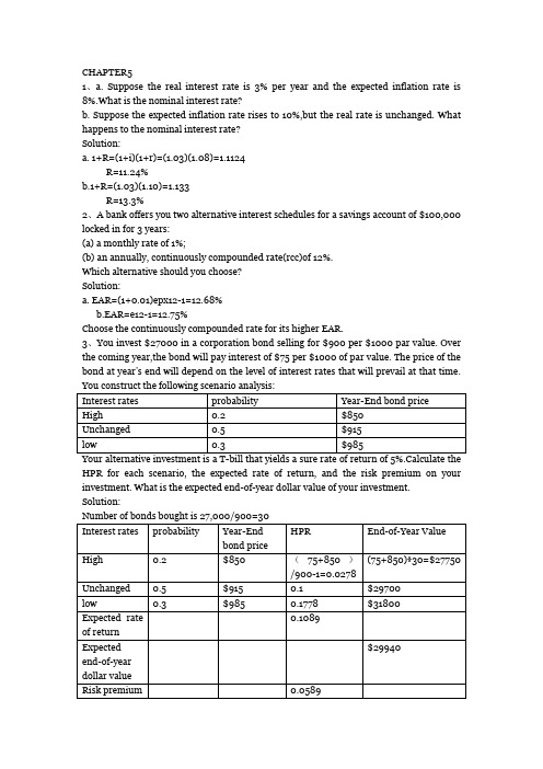
CHAPTER51、a. Suppose the real interest rate is 3% per year and the expected inflation rate is 8%.What is the nominal interest rate?b. Suppose the expected inflation rate rises to 10%,but the real rate is unchanged. What happens to the nominal interest rate?Solution:a. 1+R=(1+i)(1+r)=(1.03)(1.08)=1.1124R=11.24%b.1+R=(1.03)(1.10)=1.133R=13.3%2、A bank offers you two alternative interest schedules for a savings account of $100,000 locked in for 3 years:(a) a monthly rate of 1%;(b) an annually, continuously compounded rate(rcc)of 12%.Which alternative should you choose?Solution:a. EAR=(1+0.01)epx12-1=12.68%b.EAR=e12-1=12.75%Choose the continuously compounded rate for its higher EAR.3、You invest $27000 in a corporation bond selling for $900 per $1000 par value. Over the coming year,the bond will pay interest of $75 per $1000 of par value. The price of the bond at year’s end will depend on the level of interest rates that will prevail at that time.HPR for each scenario, the expected rate of return, and the risk premium on your investment. What is the expected end-of-year dollar value of your investment. Solution:4、Using the annual returns for year 2003-2005 in Spreadsheet5.2,a. Compute the arithmetic average return.b. Compute the geometric average return.c. Compute the standard deviation of returns.d. compute the Sharpe ratio assuming the risk-free rate was 6% per year.Solution:a. Arithmetic return=(1/3)(0.2869)+ (1/3)(0.1088)+ (1/3)(0.0491)=14.83%;b. Geometric return= 3 0.2869*0.1088*0.0491-1=14.39%;c. Standard deviation=12.37%;d. Sharpe ratio=(14.83-6.0)/12.37=0.71;5、What is the probability that the return on the index in Example 5.10 will be below -15%?Solution:The probability of a more extreme bad month, with return below -15%,is much lower: NORMDIST(-15,1,6,TRUE)=0.00383.Alternatively,we can note that -15% is 16/6 standard deviations below the mean return, and the standard normal function to compute NORMSDIST(-16/6)=0.003836、Estimate the skew and kurtosis of the five rates in Spreadsheet 5.2.Solution:If the probability in Spreadsheet 5.2 represented the true return distribution, we would obtain:Skew=E[r(s)-E(r)]3/σ3=0.0931,Kurtosis=E[r(s)-E(r)]4/σ4-3=-1.2081Chapter61 Assume that dollar-denominated T-bills in the United States and pound-denominated bills in the United Kingdom offer equal yields to maturity. Both are short-term assets, and both are free of default risk. Neither offers investors a risk premium. However, a U.S. investor who holds U.K. bills is subject to exchange rate risk, because the pounds earned on the U.K. bills eventually will be exchanged for dollars at the future exchange rate. Is the U.S. investor engaging in speculation or gambling?The investor is taking on exchange rate risk by investing in a pound-denominated asset. If the exchange rate moves in the investor’s favor, the investor will benefit and will earn more from the U.K. bill than the U.S. bill. For example, if both the U.S. and U.K. interest rates are 5%, and the current exchange rate is $2 per pound, a $2 investment today can buy 1 pound, which can be invested in England at a certain rate of 5%, for a year-end value of 1.05 pounds. If the year-end exchange rate is $2.10 per pound, the 1.05 pounds can be exchanged for 1.05 ×$2.10 =$2.205for a rate of return in dollars of 1+r = $2.205/$2 = 1.1025, or r = 10.25%, more than is available from U.S. bills. Therefore, if the investor expects favorable exchange rate movements, the U.K. bill is a speculative investment. Otherwise, it is a gamble.2 A portfolio has an expected rate of return of 20% and standard deviation of 30%. T-bills offer a safe rate of return of 7%. Would an investor with risk-aversion parameter A=4 prefer to invest in T-bills or the risky portfolio? What if A =2?For the A =4 investor the utility of the risky portfolio isU = .20 -( ½×4× .32) =.02while the utility of bills isU = .07 - ( ½×4 ×0) = .07The investor will prefer bills to the risky portfolio. (Of course, a mixture of bills and the portfolio might be even better, but that is not a choice here.)Even for the A =2 investor, the utility of the risky portfolio isU =.20 - ( ½× 2 × .32) = .11while the utility of bills is again .07. The less risk-averse investor prefers the risky portfolio.3.a. How will the indifference curve of a less riskaverse investor compare to the indifference curve drawn in Figure 6.2?b. Draw both indifference curves passing through point P.The less risk-averse investor has a shallower indifference curve. An increase in risk requires less increase in expected return to restore utility to the original level.4What will be the dollar value of your position in equities (E), and its proportion in your overall portfolio, if you decide to hold 50% of your investment budget in Ready Asset? Holding 50% of your invested capital in Ready Assets means that your investment proportion inthe risky portfolio is reduced from 70% to 50%.Your risky portfolio is constructed to invest 54% in E and 46% in B. Thus the proportion of E in your overall portfolio is .5 ×54% = 27%, and the dollar value of your position in E is$300,000 × .27 =$81,000.5. Can the reward-to-volatility (Sharpe) ratio, S =[E(rC) _ rf]/δC , of any combination of the risky asset and the risk-free asset be different from the ratio for the risky asset taken alone,[E(rP) -rf]/δP , which in this case is .36?In the expected return–standard deviation plane all portfolios that are constructed from the same risky and risk-free funds (with various proportions) lie on a line from the risk-free rate through the risky fund. The slope of the CAL (capital allocation line) is the same everywhere; hence the reward-to-volatility ratio is the same for all of these portfolios. Formally, if you invest a proportion, y, in a risky fund with expected return E ( r P ) and standard deviation δP, and the remainder, 1 -y, in a risk-free asset with a sure rate r f , then the portfolio’s expected return andstandard deviation areE(rC) = rf +y[E(rP) - rf]δC = yδPVisit us and therefore the reward-to-volatility ratio of this portfolio isSC =﹙E(rC)- rf﹚/δC=y[E(rP)- rf]/yδP=﹙E(rP)- rf﹚/δPwhich is independent of the proportion y.6.Suppose that there is an upward shift in the expected rate of return on the risky asset, from 15% to 17%. If all other parameters remain unchanged, what will be the slope of the CAL fory ≤1 and y > 1?The lending and borrowing rates are unchanged at rf =7%, r fB =9%. The standard deviation of the risky portfolio is still 22%, but its expected rate of return shifts from 15% to 17%.The slope of the two-part CAL is﹙E(rP)- rf﹚/δP for the lending range﹙E(rP) - r fB﹚/δP for the borrowing rangeThus in both cases the slope increases: from 8/22 to 10/22 for the lending range, and from 6/22 to 8/22 for the borrowing range.7. a. If an investor’s coefficient of risk aversion i s A= 3, how does the optimal asset mix change? What are the new values of E(rC) and δC?b. Suppose that the borrowing rate, r f B =9% is greater than the lending rate, rf =7%. Show graphically how the optimal portfolio choice of some investors will be affected by the higher borrowing rate. Which investors will not be affected by the borrowing rate? a. The parameters are r f = .07, E ( r P ) =.15, δP = .22. An investor with a degree of risk aversionA will choose a proportion y in the risky portfolio ofy =﹙E(rP)-rf﹚/AδP²With the assumed parameters and with A = 3 we find thaty =﹙.15- .07﹚/﹙3 × .0484﹚=.55When the degree of risk aversion decreases from the original value of 4 to the new value of 3,investment in the risky portfolio increases from 41% to 55%. Accordingly, theexpected return and standard deviation of the optimal portfolio increase:E(rC) =.07 +(.55 × .08) = .114 (before: .1028)δC = .55 × .22 =.121 (before: .0902)b. All investors whose degree of risk aversion is such that they would hold the risky portfolio in a proportion equal to 100% or less ( y < 1.00) are lending rather than borrowing, and so are unaffected by the borrowing rate. The least risk-averse of these investors hold 100% in the risky portfolio ( y =1). We can solve for the degree of risk aversion of these “cut off” investors from the parameters of the investment opportunities: y =1 =﹙E(rP)- rf﹚/A P²=.08/.0484 Awhich impliesA =.08/.0484=1.65Any investor who is more risk tolerant (that is, A < 1.65) would borrow if the borrowing ratewere 7%. For borrowers,y =﹙E(rP) -r f B﹚/A P²Suppose, for example, an investor has an A of 1.1. When rf =r fB =7%, this investor chooses to invest in the risky portfolio:y =.08/﹙1.1×.0484﹚=1.50which means that the investor will borrow an amount equal to 50% of her own investment capital. Raise the borrowing rate, in this case to r fB =9%, and the investor will invest less in the risky asset. In that case:y= .06/﹙1.1× .0484﹚=1.13and “only” 13% of her investment capital will be borrowed. Graphically, the line from r f to the risky portfolio shows the CAL for lenders. The dashed part would be relevant if the borrowing rate equaled the lending rate. When the borrowing rate exceeds the lending rate, the CAL is kinked at the point corresponding to the risky portfolio.The following figure shows indifference curves of two investors. The steeper indifference curve portrays the more risk-averse investor, who chooses portfolio C 0 , which involves lending. This investor’s choice is unaffected by the borrowing rate. The more risk-tolerant investor is portrayed by the shallower-sloped indifference curves. If the lending rate equaled the borrowing rate, this investor would choose portfolio C 1 on the dashed part of the CAL. When the borrowing rate goes up, this investor chooses portfolio C 2 (in the borrowing range of the kinked CAL), which involves less borrowing than before. This investor is hurt by the increase in the borrowing rate.8. Suppose that expectations about the S&P 500 index and the T-bill rate are the same as they were in 2005, but you find that a greater proportion is invested in T-bills today than in 2005.What can you conclude about the change in risk tolerance over the years since 2005?If all the investment parameters remain unchanged, the only reason for an investor to decrease the investment proportion in the risky asset is an increase in the degree of risk aversion. If you think that this is unlikely, then you have to reconsider your faith in your assumptions. Perhaps the S&P 500 is not a good proxy for the optimal risky portfolio. Perhaps investors expect a higher real rate on T-bills.第七章concept checkPortfolio weight WD WEWD COV(rd,rd) COV(rd,re)WE COV(re.,rd) COV(re,re)用行列乘以对应因子,可得σp2=WD2COV(rd,rd)+WDWECOV(rd,re)+WEWD COV(re.,rd)+WE2 COV(re,re). 因为COV(rd,rd)= σDσDρDD,ρDD=1,所以COV(rd,rd)= σD2。
absolute risk aversion计算
absolute risk aversion计算Absolute risk aversion(绝对风险厌恶)是金融领域中的一个重要概念,用于衡量投资者对风险的厌恶程度。
它反映了投资者在面临收益和风险时,更倾向于选择稳定的收益,即使这意味着放弃潜在的高收益。
在本文中,我们将详细介绍如何计算绝对风险厌恶(Absolute risk aversion)。
1. 定义绝对风险厌恶(Absolute risk aversion)绝对风险厌恶是指投资者在面临两种投资选择时,更倾向于选择具有较低绝对风险的投资。
换句话说,投资者愿意放弃一定的预期收益以降低投资组合的波动性。
绝对风险厌恶可以通过以下公式计算:绝对风险厌恶(Absolute risk aversion)= (预期收益- 无风险资产收益) / 投资组合的波动性其中,预期收益是指投资者期望从投资中获得的收益,无风险资产收益是指投资者投资无风险资产(如国债)所获得的收益。
投资组合的波动性是指投资组合中资产价格波动的程度。
1. 计算步骤假设投资者正在考虑两种投资选择:投资A和投资B。
投资A的预期收益为10%,投资B的预期收益为12%。
同时,投资A的波动性为15%,投资B的波动性为20%。
无风险资产的收益为4%。
首先,我们需要计算投资A和投资B的绝对风险厌恶:投资A的绝对风险厌恶= (10% - 4%) / 15% = 0.2投资B的绝对风险厌恶= (12% - 4%) / 20% = 0.3由此可见,投资B的绝对风险厌恶值更高,说明投资者对投资B的风险更敏感。
因此,在面临投资选择时,投资者可能会选择投资A,因为它具有较低的绝对风险厌恶。
1. 应用绝对风险厌恶(Absolute risk aversion)绝对风险厌恶可以帮助投资者在面临投资选择时,更好地了解自己的风险偏好。
通过计算不同投资的绝对风险厌恶值,投资者可以找到具有较低风险的投资选择,从而实现投资组合的优化。
经典资产定价理论综述
Financial View | 金融视线MODERN BUSINESS现代商业156经典资产定价理论综述肖琨小 中央财经大学金融学院 北京 100081摘要:本文从威廉·夏普提出的CAPM模型出发,指出其在理论与实证中的不足,从而从三个不同发展方向出发,全面梳理资产定价深化研究,逐步引入CAPM模型的各种拓展模型,从而较为全面的介绍经典的资本资产定价相关理论。
关键词:资本资产定价;APT模型;CCAPM模型;行为金融理论一、引言资本资产的定价问题一直深受金融市场领域乃至整个金融领域的关注。
研究最早起源于20世界50年代,随着经济、金融的不断发展,如今,如何有效的确定金融资产的价格仍是很多经济学家所面临的重大问题。
马科威茨通过把收益、风险分别定义为均值和方差,第一次从数量上解决了收益与风险的关系问题,资本资产定价模型就是在这一理论的基础之上提出的。
1970年,威廉·夏普率先提出资本资产定价模型:CAPM模型,成为资本资产定价的基础。
它的结论非常简单:投资的收益只与风险有关。
虽然,CAPM模型的提出非常成功,但还是存在着很多理论上、实践上的局限性。
首先,C A P M 的假设前提难以实现;其次,CAPM中的β值难以确定;最后,与之相关的实证结果令人失望。
因此,金融市场学家不断探求比CAPM更为有效的资本市场理论。
经济学家们大致从三个方面进行了改进:第一、将单因素CAPM拓展为多因素模型,如APT套利定价理论,Fama-French 三因素模型(提出SMB和 HML因素);第二、提出基于消费的CCAPM模型,将资产回报率与宏观经济变量联系起来;第三,由行为金融学理论对资产定价问题进行解释。
二、资本资产定价的多因素模型(一)套利定价理论APT该模型由斯蒂芬·罗斯于1976年提出,与CAMP模型相比,其最大的特点是利用套利概念定义均衡,并且该模型的假设更加合理。
套利定价理论的基本机制是:在均衡市场中,两种相同的商品必定以相同价格出售。
人格类型、任务特征对风险决策行为的影响
摘要人们在日常生活中,到处都面临着各种各样的决策,人生就是一个不断决策的过程。
风险决策作为决策的一个类别,已经成为众多学科研究的热点。
本研究首先按照决策理论发展过程中一些经典悖论的提出和解释为脉络,对当今的风险决策理论进行简要的回顾。
然后分析影响风险决策的主要因素,其中包括任务特征因素和个体因素。
任务特征因素包括任务框架、风险情境和概率水平三种。
本研究重点想探究个体因素中的人格对风险决策行为的影响。
以MBTl人格理论为框架,采用实验法和测验法相结合的方法进行研究。
研究结果表明:(1)人格作为个体因素对风险决策有影响。
对人格维度得分和风险决策行为进行分析时,不同人格维度对决策的影响不一致。
其中感觉直觉维度得分高的被试偏向于保守选择。
(2)决策任务特征中的任务框架,概率水平,和风险情境的主效应作用均显著。
在正框架,投资盈利情境中,被试多表现出对保守的偏爱:在负框架,投资损失和煤矿爆炸涉及抢救生命的问题时,被试对冒险的偏好达到非常显著的水平。
概率水平与框架和风险情境之间的交互作用也显著。
(3)当对不同人格维度被试在冒险和保守选择的频次进行分析时。
人格维度中的内外倾维度,感觉直觉维度,和思考情感维度与任务特征中的正负框架之间的交互作用显著,内外倾维度与思考情感维度都与风险情境和框架之间存在交互作用,思考情感维度与任务特征的三因素交互作用显著。
关键词:人格类型;风险决策;船TI;框架;风险情境;概率水平AbstractIn o u r dai ly life,people a r e ar e faced with a w ide range of decis ion.m aking everywhere.and life is a continuous process of decision.making.As a typ e of decision.making,risk d ecision—making has be c o me a hotspot and foCUS a c r o s s man y subjects.At frist of this s tudy,we u s e th e classic para d ox’S pr op os e and interpret as a c o n te x t t o expound the deve lop men t of t he t heory of decisi on.making.And th en we clarified two charaeteristic factors influencing risk decision—making.One is c ha rac te rs of d ec i s io n-m a k in g task and th e o the r is i ndi vidu al factors.The charact er of decision.making ta sk inclu des risk situation,task fr am e and pro bab ilit y le vel.th e focus of01117study want to explore the i nfl uen ces of person ality types o n de cisio n—m aking behavi or.in the framework of MBTI personality theory,using the c o mb in a ti o n of experimental method and th e m easureme nt method.The results of the re se arc h in di ca t es that:(1)Personality a s o n e of ind ivi dua l risk factors affect the decision-making.whenwe analysis the s c o r e s o n the personality di mens ion and risk decision-making behavior.Different pers onal ity di me ns io ns h as a in con si ste nt impac t o ndecision-making.Those w h o has a hi曲scores o nSensing.iNtuition dimensio n tend to choose the conservative optio n.(2)TlH.ee ta sk c h ar a ct er i st i es a r e all h av e main e侬ct.in p osi tiv e framework and,the test showed m or e pref erence o n a conservatism;in negative f r am e wo rk,i nv e s t me n t in a losses situation and mine explosion involving the issueof ’s avi ng lives,the prefer o f risk—taking get a very significantle ve l.P ro ba b il i ty levels and risk si tu a ti on s significantly influenc e risk deci sion.making ininteractive efreet.(3)Whe n we a nal ys is t he frequency of the personality d im en si on of differentsubjects in the risk-ta king and conser vative choice,the External.Internald ime n s io n s、S e n si n g.i n t u it i o n d ime nsi on and Thinki ng.Feeling di me nsi onare all ha ve a interactive effect with the framework.the External.Internaldi me n si o ns and T hi n k in g-F ee l i n g d ime nsi on ha ve a interactive effect with framework and risk situatio ns.Thinking.Feeling di men sio n have ainteractive effect wit h all o f the t hree tas k characteristics.K e y words:Personality type;Risk decision-making;MBTI,Frame;Risk situations;Probabi lity levelⅡ独创性声明本人郑重声明:所提交的学位论文是本人在导师指导下独立进行研究工作所取得的成果。
前景理论——精选推荐
前景理论的数学模型前景理论⽬录[ 隐藏 ]1简介2理论的产⽣3理论内涵4数学模型4.1举例5引申的四个基本结论6实例7缺陷 前景理论(英⽂:prospect theory,也作展望理论、预期理论),是⼀个⾏为经济学的理论,为⼼理学教授丹尼尔·卡内曼(Daniel Kahneman)和阿摩司·特沃斯基(Amos Tversky)提出的。
这个理论的假设之⼀是,每个⼈基于初始状况(参考点位置)的不同,对风险会有不同的态度。
它与锚定效应、泰勒的“⼼理账户”原理共同构成⾏为经济学的三⼤基⽯;与后悔理论(Regret Theory)、过度反应理论(Overreaction Theory)及过度⾃信理论(Overconfidence Theory)被誉为⾦融学的四⼤研究成果。
它的作者之⼀丹尼尔·卡内曼因此获得2002年的诺贝尔经济学奖。
编辑本段简介 前景理论是描述性范式的⼀个决策模型,它假设风险决策过程分为编辑和评价两个过程。
在编辑阶段,个体凭借“框架”(frame)、参照点(reference point)等采集和处理信息,在评价阶段依赖价值函数(value function)和(主观概率)的权重函数(weighting function)对信息予以判断。
在价值函数是经验型的,它有三个特征,⼀是⼤多数⼈在⾯临获得时是风险规避的;⼆是⼤多数⼈在⾯临损失时是风险偏爱的;三是⼈们对损失⽐对获得更敏感。
因此,⼈们在⾯临获得时往往是⼩⼼翼翼,不愿冒风险;⽽在⾯对失去时会很不⽢⼼,容易冒险。
⼈们对损失和获得的敏感程度是不同的,损失时的痛苦感要⼤⼤超过获得时的快乐感。
此理论是⾏为经济学的重⼤成果之⼀。
1970年代,卡内曼和特沃斯基系统地研究这⼀领域。
长久以来,主流经济学都假设每个⼈作决定时都是“理性”的,然⽽现实情况并不如此;⽽前景理论加⼊了⼈们对赚蚀、发⽣机率⾼低等条件的不对称⼼理效⽤,成功解释了许多看来不理性的现象。
- 1、下载文档前请自行甄别文档内容的完整性,平台不提供额外的编辑、内容补充、找答案等附加服务。
- 2、"仅部分预览"的文档,不可在线预览部分如存在完整性等问题,可反馈申请退款(可完整预览的文档不适用该条件!)。
- 3、如文档侵犯您的权益,请联系客服反馈,我们会尽快为您处理(人工客服工作时间:9:00-18:30)。
Risk A version and Expected-Utility Theory:A Calibration TheoremMatthew RabinDepartment of EconomicsUniversity of California–BerkeleyFirst draft distributed:October13,1997Current draft:May29,1999AbstractWithin the expected-utility framework,the only explanation for risk aversion is thatthe utility function for wealth is concave:A person has lower marginal utility for addi-tional wealth when she is wealthy than when she is poor.This paper provides a theoremshowing that expected-utility theory is an utterly implausible explanation for apprecia-ble risk aversion over modest stakes:Within expected-utility theory,for any concaveutility function,even very little risk aversion over modest stakes implies an absurddegree of risk aversion over large stakes.Illustrative calibrations are provided.Keywords:Diminishing Marginal Utility,Expected Utility,Risk A versionJEL Classifications:B49,D11,D81Acknowledgments:Many people,including David Bowman,Colin Camerer,Eddie Dekel,Larry Epstein,Erik Eyster,Mitch Polin-sky,Drazen Prelec,Richard Thaler,and Roberto W eber,as well as Andy Postlewaite and two anonymous referees,have provided useful feedback on this paper.I thank Jimmy Chan,Erik Eyster,Roberto W eber,and especially Steven Blatt for research assistance, and the Russell Sage,MacArthur,National Science(A ward9709485),and Sloan Foundations for financial support.I also thank the Center for Advanced Studies in Behavioral Sciences,supported by NSF Grant SBR-960123,where an earlier draft of the paper was written.Mail:549Evans Hall#3880/Department of Economics/University of California,Berkeley/Berkeley,CA94720-3880.E-mail: rabin@.CB Handle:‘‘Game Boy’’.W eb Page:/~rabin/index.html1.IntroductionUsing expected-utility theory,economists model risk aversion as arising solely because the utility function over wealth is concave.This diminishing-marginal-utility-of-wealth theory of risk aver-sion is psychologically intuitive,and surely helps explain some of our aversion to large-scale risk: W e dislike vast uncertainty in lifetime wealth because a dollar that helps us avoid poverty is more valuable than a dollar that helps us become very rich.Y et this theory also implies that people are approximately risk neutral when stakes are small. Arrow(1971,p.100)shows that an expected-utility maximizer with a differentiable utility function will always want to take a sufficiently small stake in any positive-expected-value bet.That is, expected-utility maximizers are(almost everywhere)arbitrarily close to risk neutral when stakes are arbitrarily small.While most economists understand this formal limit result,fewer appreciate that the approximate risk-neutrality prediction holds not just for negligible stakes,but for quite sizable and economically important stakes.Economists often invoke expected-utility theory to explain substantial(observed or posited)risk aversion over stakes where the theory actually predicts virtual risk neutrality.While not broadly appreciated,the inability of expected-utility theory to provide a plausible account of risk aversion over modest stakes has become oral tradition among some subsets of re-searchers,and has been illustrated in writing in a variety of different contexts using standard utility functions.1In this paper,I reinforce this previous research by presenting a theorem which cali-brates a relationship between risk attitudes over small and large stakes.The theorem shows that, within the expected-utility model,anything but virtual risk neutrality over modest stakes implies manifestly unrealistic risk aversion over large stakes.The theorem is entirely‘‘non-parametric’’, assuming nothing about the utility function except concavity.In the next section I illustrate implications of the theorem with examples of the form‘‘If an expected-utility maximizer always turns down modest-stakes gamble X,she will always turn down large-stakes gamble Y.’’Suppose that,from any initial wealth level,a person turns down gambles where she loses$100or gains$110,each with50%probability.Then she will turn down50-50bets"See Epstein(1992),Epstein and Zin(1990),Hansson(1988),Kandel and Stambaugh(1991),Loomes and Segal (1994),and Segal and Spivak(1990).Hansson’s(1988)discussion is most similar to the themes raised in this paper. He illustrates how a person who for all initial wealth levels is exactly indifferent between gaining$7for sure and a 50-50gamble of gaining either$0or$21prefers a sure gain of$7to any lottery where the chance of gaining positive amounts of money is less than40%–no matter how large the potential gain is.of losing$1,000or gaining any sum of money.A person who would always turn down50-50lose $1,000/gain$1,050bets would always turn down50-50bets of losing$20,000or gaining any sum. These are implausible degrees of risk aversion.The theorem not only yields implications if we know somebody will turn down a bet for all initial wealth levels.Suppose we knew a risk-averse person turns down50-50lose$100/gain$105bets for any lifetime wealth level less than$350,000, but knew nothing about the degree of her risk aversion for wealth levels above$350,000.Then we know that from an initial wealth level of$340,000the person will turn down a50-50bet of losing $4,000and gaining$635,670.The intuition for such examples,and for the theorem itself,is that within the expected-utility framework turning down a modest-stakes gamble means that the marginal utility of money must diminish very quickly for small changes in wealth.For instance,if you reject a50-50lose$10/gain $11gamble because of diminishing marginal utility,it must be that you value the11th dollar above your current wealth by at most fas much as you valued the10| -to-last-dollar of your current wealth.2Iterating this observation,if you have the same aversion to the lose$10/gain$11bet ifyou were$21wealthier,you value the32?_dollar above your current wealth by at most ffDS as much as your10| -to-last dollar.Y ou will value your220th dollar by at most2fas muchas your last dollar,and your880| dollar by at most2c fffof your last dollar.This is an absurd rate for the value of money to deteriorate—and the theorem shows the rate of deterioration implied by expected-utility theory is actually quicker than this.Indeed,the theorem is really just an algebraic articulation of how implausible it is that the consumption value of a dollar changes significantly as a function of whether your lifetime wealth is$10,$100,or even$1,000higher or lower.From such observations we should conclude that aversion to modest-stakes risk has nothing to do with the diminishing marginal utility of wealth.Expected-utility theory seems to be a useful and adequate model of risk aversion for many pur-poses,and it is especially attractive in lieu of an equally tractable alternative model.‘‘Extremely-concave expected utility’’may even be useful as a parsimonious tool for modeling aversion to modest-scale risk.But this and previous papers make clear that expected-utility theory is mani-#My wording here,as in the opening paragraph and elsewhere,gives a psychological interpretation to the concavity of the utility function.Y et a referee has reminded me that a common perspective among economists studying choice under uncertainty has been that the concavity of the utility function need be given no psychological interpretation.I add such psychological interpretation throughout the paper as an aid to those readers who,like me,find this approach to be the natural way to think about utility theory,but of course the mathematical results and behavioral analysis in this paper hold without such interpretations.festly not close to the right explanation of risk attitudes over modest stakes.Moreover,when the specific structure of expected-utility theory is used to analyze situations involving modest stakes —such as in research that assumes that large-stake and modest-stake risk attitudes derive from the same utility-for-wealth function —it can be very misleading.In the concluding section,I discuss a few examples of such research where the expected-utility hypothesis is detrimentally maintained,and speculate very briefly on what set of ingredients may be needed to provide a better account of risk attitudes.In the next section,I discuss the theorem and illustrate its implications.2.Some Calibrations Based on a TheoremConsider an expected-utility maximizer over wealth, ,with V on Neumann-Morgenstern prefer-ences L E .Assume that the person likes money and is risk-averse:For all ,L E is (strictly)increasing and (weakly)concave.Suppose further that,for some range of initial wealth levels and for some }:,:f ,she will reject bets losing $,or gaining $},each with 50%chance.3From the assumption that these bets will be rejected,the theorem presented in this paper places an upper bound on the rate at which utility increases above a given wealth level,and a lower bound on the rate at which utility decreases below that wealth level.Its proof is a short series of algebraic ma-nipulations;both the theorem and proof are in the appendix.Its basic intuition is straightforward,as described briefly in the introduction.The theorem handles cases where we know a person to be averse to a gamble only for some ranges of initial wealth.A simpler corollary,also in the appendix,holds when we know a lower bound on risk aversion for all wealth levels.T able 1illustrates some of the corollary’s implications:Consider an individual who is known to reject,for all initial wealth levels,50-50,lose $100/gain }bets,for }'m f ,m fD ,m f ,and m 2D .The table presents implications of the form ‘‘the person will turn down 50-50gambles of losing u and gaining C ,’’where each u is a row in the table and the highest C (using the bounds established by the corollary)making the statement true is the entry $The assumption that :is concave is not implied by the fact that an agent always turns down a given better-than-fair bet;if you know that a person always turns down 50-50lose $10/gain $11bets,you don’t know that her utility function is concave everywhere –it could be convex over small ranges.(For instance,let :+z ,@4 "# z for z @#+4<3>533,,but X +z ,@4 45 4<.k 45 4< "# #!l +z 4<,#for z #+4<3>533,.)Concavity is an additional assumption,but I am confident that results hold approximately if we allow such small and silly non-convexities.in the table 4All entries are rounded down to an even dollar amount.jO$101$105$110$125$4004004205501,250$600600730990"$8008001,0502,090"$1,0001,0101,570""$2,0002,320"""$4,0005,750"""$6,00011,810"""$8,00034,940"""$10,000""""$20,000""""Wdeoh4If averse to50-50lose$100/gain j bets for all wealth levels,will turn down50-50lose O/gain J bets;J’s entered in table.So,for instance,if a person always turns down a50-50lose m ff/gain m f gamble,she will always turn down a50-50lose$800/gain$2,090gamble.Entries of"are literal:Somebody who always turns down50-50lose$100/gain$125gambles will turn down any gamble with a50% chance of losing$600.This is because the fact that the bound on risk aversion holds everywhere implies that L E is bounded above.The theorem and corollary are homogenous of degree1:If we know that turning down50-50 lose,/gain}gambles implies you will turn down50-50lose u/gain C,then for all%:f,turning down50-50lose%,/gain%}gambles implies you will turn down50-50lose%u/gain%C.Hence the u'm f c fff,}'m f entry in T able1tells us that turning down50-50lose m f/gain$10.10 gambles implies you will turn down50-50lose$1,000/gain"gambles.The reader may worry that the extreme risk aversion shown in T able1relies heavily on the assumption that the person will turn down the given gamble for all initial wealth levels.It doesn’t. While without knowing a global lower bound on a person’s modest-stakes risk aversion we cannot assert that she’ll turn down gambles with infinite expected return,T able2indicates that the lack of a lower bound does not salvage the plausibility of expected-utility theory.T able2shows calibrations if we know the person will turn down50-50lose$100/gain}gambles for initial wealth levels %The theorem provides a lower bound on the concavity of the utility function,and its proof indicates an obvious way to obtain a stronger(but uglier)result.Also,while the theorem and applications focus on‘‘50-50bets’’,the point is applicable to more general bets.For instance,if an expected-utility maximizer dislikes a bet with a25%chance of losing$100an a75%chance of winning$100,then she would turn down50-50lose$100/gain$300bets,and we could apply the theorem from there.less than$300,000,indicating which gambles she’ll turn down starting from initial wealth level of $2bf c rge entries are approximate.jO$101$105$110$125$4004004205501,250$60060073099036,000,000,000$8008001,0502,09090,000,000,000$1,0001,0101,570718,190160,000,000,000$2,0002,32069,93012,210,880850,000,000,000$4,0005,750635,67060,528,9309,400,000,000,000$6,00011,5101,557,360180,000,00089,000,000,000,000$8,00019,2903,058,540510,000,000830,000,000,000,000$10,00027,7805,503,7901,300,000,0007,700,000,000,000,000$20,00085,75071,799,110160,000,000,000540,000,000,000,000,000,000Wdeoh5T able1replicated,for initial wealth level$290,000,wheno@j behavior is only known to hold for z $!!>!!!.If we only know that a person turns down50-50lose$100/gain$125bets when her lifetime wealth is below$300,000,we also know she will turn down a50-50lose$600/gain$36billion bet beginning from lifetime$290,000.5The intuition is that the extreme concavity of the utility function between$290,000and$300,000assures that the marginal utility at$300,000is tiny compared to the marginal utility at wealth levels below$290,000;hence,even if the marginal utility does not diminish at all above$300,000,a person won’t care nearly as much about money above$300,000 as she does about amounts below$290,000.The choice of$290,000and$300,000as the two focal wealth levels is arbitrary;all that matters is that they are$10,000apart.As with T able1,T able2 is homogenous of degree1,where the wedge between the two wealth levels must be multiplied by the same factor as the other entries.Hence—multiplying T able2by10—if an expected-utility maximizer would turn down a50-50lose$1,000/gain$1,050gamble whenever her lifetime wealth is below$300,000,then from an initial wealth level of$200,000she will turn down a50-50lose $40,000/gain$6,356,700gamble.While these‘‘non-parametric’’calibrations are less conducive to analyzing more complex ques-tions,T able3provides similar calibrations for decisions that resemble real-world investment choices &Careful examination of T ables1and2show that most entries that are not"in T able1show up exactly the same in T able2.The two exceptions are those entries that are above$10,000—since T able2implicitly makes no assumptions about concavity for gains of more than$10,000,it yields lower numbers.by assuming conventional functional forms of utility functions.It shows what aversion to various gambles implies for the maximum amount of money a person with a constant-absolute-risk-aversion (CARA)utility function would be willing to keep invested in the stock market,for reasonable as-sumptions about the distribution of returns for stocks and bonds.o@j [$100/$101.0000990$14,899$100/$105.0004760$3,099$100/$110.0009084$1,639$100/$125.0019917$741$100/$150.0032886$449$1,000/$1,050.0000476$30,987$1,000/$1,100.0000908$16,389$1,000/$1,200.0001662$8,886$1,000/$1,500.0003288$4,497$1,000/$2,000.0004812$3,067$10,000/$11,000.0000090$163,889$10,000/$12,000.0000166$88,855$10,000/$15,000.0000328$44,970$10,000/$20,000.0000481$30,665Wdeoh6If a person has CARA utility function and is averse to&!@&!lose$o/gain$j bets for all wealth levels,then 1)she has coefficient of absolute risk aversion no smaller than and2)invests$[in the stock market when stock yields are normally distributed with mean real return'=% and standard deviation#! >andbonds yield a riskless return of!=& .Hence,an expected-utility maximizer with CARA preferences who turns down50/50lose$1,000/gain $1,200gambles will only be willing to keep$8,875of her portfolio in the stock market,no matter how large her total investments in stocks and bonds.If she turns down a50/50lose$100/gain$110 bet,she will be willing to keep only$1,600of her portfolio in the stock market—keeping the rest in bonds(which average6%lower annual return).While it is widely believed that investors are too cautious in their investment behavior,no one believes they are this risk averse.3.Discussion and ConclusionExpected-utility theory may well be a useful model of the taste for very-large-scale insurance.6 Despite its usefulness,however,there are reasons why it is important for economists to recognize 9While there is also much evidence for some limits of its applicability for large-scale risks,and the results of this paper suggest an important flaw with the expected-utility model,the specific results do not of course demonstrate that the model is unuseful in all domains.how miscalibrated expected-utility theory is as an explanation of modest-scale risk aversion.For instance,some research methods economists currently employ should be abandoned because they rely crucially on the expected-utility interpretation of modest-scale risk aversion.One example arises in experimental economics.In recent years,there has been extensive laboratory research in economics in which subjects interact to generate outcomes with payoffs on the order of$10to$20. Researchers are often interested in inferring subjects’beliefs from their behavior.Doing so often requires knowing the relative value subjects hold for different money prizes;if a person chooses$5 in event A over$10in event B,we know that she believes A is at least twice as likely as B only if we can assume the person likes$10at least twice as much as$5.Y et economic theory tells us that, because of diminishing marginal utility of wealth,we should not assume people like$10exactly twice as much as$5.Experimentalists(e.g.,Davis and Holt(1993,pp.472-6))have developed a clever scheme to avoid this problem:Instead of prizes of$10and$5,subjects are given prizes such as10%chance of winning$100vs.5%chance of winning$100.Expected-utility theory tells us that,irrespective of the utility function,a subject values the10%chance of a prize exactly twice as much as the5%chance of winning the same prize.The problem with this lottery procedure is that it is known to be sufficient only when we main-tain the expected-utility hypothesis.But then it is not necessary—since expected-utility theory tells us that people will be virtually risk neutral in decisions on the scale of laboratory stakes.If expected-utility theory is right,these procedures are at best redundant,and are probably harmful.7 On the other hand,if we think that subjects in experiments are risk averse,then we know they are not expected-utility maximizers.Hence the lottery procedure,which is motivated solely by expected-utility theory’s assumptions that preferences are linear in probabilities and that risk atti-tudes come only from the curvature of the utility-of-wealth function,has little presumptive value in‘‘neutralizing’’risk aversion.Perhaps there are theories of risk attitudes such that the lottery:If expected-utility theory explained behavior,these procedures would surely not be worth the extra expense,nor the loss in reliability of the data from making experiments more complicated.Nor should experimentalists who believe in expected utility theory ever be cautious about inferences made from existing experiments that don’t use the lottery methods out of fear that the results are confounded by the subjects’risk attitudes.procedure is useful for neutralizing risk aversion—but expected-utility theory isn’t one of them.8A second example of problematic research methods relates to the logic underlying the theorem: Expected-utility theory makes wrong predictions about the relationship between risk aversion over modest stakes and risk aversion over large stakes.Hence,when measuring risk attitudes main-taining the expected-utility hypothesis,differences in estimates of risk attitudes may come from differences in the scale of risk comprising data sets,rather than from differences in risk attitudes of the people being studied.9Data sets dominated by modest-risk investment opportunities are likely to yield much higher estimates of risk aversion than data sets dominated by larger-scale investment opportunities.So not only are standard measures of risk aversion somewhat hard to interpret given that people are not expected-utility maximizers,but even attempts to compare risk attitudes so as to compare across groups will be misleading unless economists pay due attention to the theory’s calibrational problems.The problems with assuming that risk attitudes over modest and large stakes derive from the same utility-of-wealth function relates to a long-standing debate in economics.Expected-utility theory makes a powerful prediction that economic actors don’t see an amalgamation of independent gambles as significant insurance against the risk of those gambles;they are either barely less willing or barely more willing to accept risks when clumped together than when apart.This observation was introduced in a famous article by Samuelson(1963),who showed that expected-utility theory implies that if(for some sufficiently wide range of initial wealth levels)a person turns down a particular gamble,then she should also turn down an offer to play?:Q of those gambles.Hence, in his example,if Samuelson’s colleague is unwilling to accept a50-50lose$100/gain$200gamble, then he should be unwilling to accept100of those gambles taken together.Though Samuelson’s theorem is‘‘weaker’’than the one in this paper,it makes manifest the fact that expected-utility ;Indeed,the observation that diminishing marginal utility of wealth is irrelevant in laboratory experiments raises questions about interpreting experimental tests of the adequacy of expected-utility theory.For instance,while show-ing that existing alternative models better fit experimental data than does expected-utility theory,Harless and Camerer (1994)show that expected-utility theory better fits experimental data than does‘‘expected-value theory’’—risk-neutral expected-utility theory.But because expected-utility implies that laboratory subjects should be risk neutral,such evi-dence that expected-utility theory explains behavior better than expected-value theory is evidence against expected-utility theory.<Indeed,Kandel and Stambaugh(1991,pp.68-69)discuss how the plausibility of estimates for the coefficient of relative risk aversion may be very sensitive to the scale of risk being examined.Assuming constant risk aversion, they illustrate how a coefficient of relative risk aversion needed to avoid predicting absurdly large aversion to a50/50 lose$25,000/gain$25,000gamble generates absurdly little aversion to a50/50lose$400/gain$400gamble.They summarize such examples as saying that‘‘Inferences about[the coefficient of relative risk aversion]are perhaps most elusive when pursued in the introspective context of thought experiments.’’But precisely the same problem makes inferences from real data elusive.theory predicts that adding together a lot of independent risks should not appreciably alter attitudes towards those risks.Y et virtually everybody would find the aggregated gamble of10050-50lose$100/gain$200chance bets attractive.It has an expected yield of$5,000,with negligible risk:There is only a.ffof losing any money and merely achance of losing more than$1,000.10While nobody would2D?fffturn down this gamble,many people,such as Samuelson’s colleague,might reject the single50-50 lose$100/gain$200bet.11Hence,using expected-utility theory to make inferences about the risk attitudes towards the amalgamated bet from the reaction to the one bet—or vice versa—would be misleading.What does explain risk aversion over modest stakes?While this paper provides a‘‘proof by cal-ibration’’that expected-utility theory does not help explain some risk attitudes,there are of course more direct tests showing that alternative models better capture risk attitudes.There is a large liter-ature(see Machina(1987)and Camerer(1992)for reviews)of formal models of such alternatives. Many of these models seem to provide a more plausible account of modest-scale risk attitudes, allowing both substantial risk aversion over modest stakes and non-ridiculous risk aversion over large stakes,and researchers(e.g.,Segal and Spivak(1990),Loomes and Segal(1994),Epstein and Zin(1990))have explicitly addressed how non-expected-utility theory can help account for small-stake risk aversion.Indeed,what is empirically the most firmly established feature of risk preferences,loss aver-sion,is a departure from expected-utility theory that provides a direct explanation for modest-scale risk aversion.Loss aversion says that people are significantly more averse to losses relative to the status quo than they are attracted by gains,and more generally that people’s utilities are deter-mined by changes in wealth rather than absolute levels.12Preferences incorporating loss aversion can reconcile significant small-scale risk aversion with reasonable degrees of large-scale risk aver-43The theorem in this paper predicts that,under exactly the same assumptions invoked by Samuelson,turning down a50-50lose$100/gain$200gamble implies the person turns down a50-50lose$200/gain$20,000gamble.This has an expected return of$9,900–with zero chance of losing more than$200.44As Samuelson noted,the strong statement that somebody should turn down the many bets if and only if she turns down the one is not strictly true if a person’s risk attitudes change at different wealth levels.Indeed,many researchers (e.g.,Hellwig(1995)and Pratt and Zeckhauser(1987))have explored features of the utility function such that an expected-utility maximizer might take a multiple of a favorable bet that they would turn down in isolation.But charac-terizing such instances isn’t relevant to examples of the sort discussed by Samuelson.W e know from the unwillingness to accept a50/50lose$100/gain$200gamble that Samuelson’s colleague was not an expected-utility maximizer.45Loss aversion was introduced by Kahneman and Tversky(1979)as part of the more general‘‘prospect theory’’,and is reviewed in Kahneman,Knetch,and Thaler(1991).Tversky and Kahneman(1991)and others have estimated the loss-aversion-to-gain-attraction ratio to be about2:1.sion.13A loss-averse person will,for instance,be likely to turn down the one50/50lose$100/gain $200gamble Samuelson’s colleague turned down,but will surely accept one hundred such gambles pooled together.V ariants of this or other models of risk attitudes can provide useful alternatives to expected-utility theory that can reconcile plausible risk attitudes over large stakes with non-trivial risk aversion over modest stakes.14Appendix:The Theorem and a CorollaryTheorem:Suppose that for all ,L E is strictly increasing and weakly concave.Suppose that there exists : ,}:,:f such that for all #d c o, D L E , n D L E n} L E . Then for all #d c o,for all%:f c1)If} 2,then L E L E %;A A A ?A A A =9E%5'},!Qo E if n2, % 2, 29E ! n2,5Q},!Qo En d% E n, o},&9- ! n2,o E if% n2,2)L E n% L E;A A?A A= 99-%5'f,}o E if% 99-5'f,}o E n d% o,}&99-o E if%where,letting ?|E+ denotes the smallest integer less than or equal to+,&9E% ?|%,, 99E?|%}n,and o E L E L E , .Proof of Part1of Theorem:For notational ease and without loss of generality,let o E L E L E , ' .Then clearly L E , L E 2, ,by the concavity of L E .Also,since "$While most formal definitions of loss aversion have not made explicit the assumption that people are substantially risk averse even for very small risks(but see Bowman,Minehart,and Rabin(1999)for an explicit treatment of this issue),most examples and calibrations of loss aversion imply such small-scale risk aversion."%But Kahneman and Lovallo(1993),Benartzi and Thaler(1995),and Read,Loewenstein,and Rabin(1998)argue that an additional departure from standard assumptions is implicated in many risk attitudes is that people tend to isolate different risky choices from each other in ways that lead to different behavior than would ensue if these risks were considered jointly.Samuelson’s colleague,for instance,might reject each50/50lose$100/gain$200gamble if on each of100days he were offered one such gamble,whereas he might accept all of these gambles if they were offered to him at once.Benartzi and Thaler(1995)argue that a related type of myopia is an explanation for the‘‘equity premium puzzle’’—the mystery about the curiously large premium on returns that investors seem to demand to compensate for riskiness associated with investing in stocks.Such risk aversion can be explained with plausible(loss-averse)preferences—if investors are assumed to assess gains and losses over a short-run(yearly)horizon rather than the longer-term horizon for which they are actually investing.。