Computing transverse t-designs

合集下载

Simplifiedwavemodelling

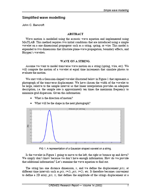
Simplified wave modellingJohn C. BancroftABSTRACTWave motion is modelled using the acoustic wave equation and implemented using MATLAB. This method requires two initial conditions that are introduced using a simple wavelet on a one dimensional propagator such as a string, spring, or wire. This model is expanded to two dimensions that illustrate plane-wave propagation, boundary effects, and Huygen’s wavelets.WAVE ON A STRING.Assume we want to model transverse wave motion on a string (spring, wire, etc). We will compute the motion of a wavelet at equal time increments that simulate photos to evaluate the motion.We start with a Gaussian-shaped wavelet illustrated below in Figure 1 that represents a photograph of the transverse displacement. We have chosen the width of the wavelet to be large, relative to the sample interval so that linear interpolation provides an adequate description, i.e. the sample rate is approximately ten times the maximum frequency to minimize grid dispersion. Given this information:•What is the direction of motion?•What will be the shape in the next photograph?FIG 1: A representation of a Gaussian shaped wavelet on a string.Is the wavelet in Figure 1 going to move to the left, the right or bounce up and down? We simply don’t know because we don’t have enough information. How do we provide that additional information? Let’s examine the wave equation to find out.The string has one distance dimension, x, and we define the displacement p(x), at different time intervals such as p(x, t=1), p(x, t=2), etc. It therefore becomes convenient to define a 2D array, p(x, t), that defines the amplitude of the strings displacement at agiven location, x , and time, t . The movement of energy on the string is governed by the one dimensional acoustic wave-equation()()22222,,1p x t p x t x v t∂∂=∂∂. (1) We will use the finite difference method to approximate the wave-equation. A second derivative of a function, f(x), is approximated in a discrete form of f at position, n , i.e. f n , and is approximated by()211222n n n f x f f f x x δ−+∂−+=∂, (2) where the increments of f n are d x . The finite difference equation for the wave equation becomes: 1,,1,,1,,1222221i j i j i j i j i j i j p p p p p p x v tδδ−+−+−+−+=. (3) This equation can be represented in graphical form in the following figure, with the increment, i , representing distance to the left, and j , the time increment that increases vertically.FIG 2: Finite difference model of full wave-equation.We wish to compute the position of the string at a new time, given some initial condition. We will choose p i, j+1 as the unknown value in the finite-difference equation because it is a single value at a new time, giving()22,1,,11,,1,222i j i j i j i j i j i j v t p p p p p p x δδ+−−+=−−+. (4) According to this equation, we need to know the position of the string at the two previous times, j , and j-1; .i.e. the two initial conditions of the string. Shown below is thefinite-difference operator positioned at the at i th spatial location to calculate the amplitude on the string for the third time, at j=3.i-1 i+1iFIG 3: The first two initial conditions at j =1 and 2 to compute the first line of samples at j=3. If we desire to model a wave travelling down the string, then we need to start with a wavelet on the string at time j=1, and the same wavelet repeated on the string at time j=2 but moved to a new spatial location. The location on the j=2 string is critical and must have a spatial increment defined by the wave velocity, v , and the time increment, d t . These two initial conditions would also match any two sequential photos of the wave moving down the string. They are shown above, along with the finite-difference operator, illustrating the computation of the amplitudes on the string at time, j=3. (The above figure has used a very large d x on the operator for the purposes of illustration only).Computer simulations are illustrated in Figure 4, with (a) showing the amplitude of a Gaussian wavelet on the string at the first two times and the resulting calculation of the wavelet at the third time, k=3. The amplitudes at succeeding times may be calculated from the previous two times as illustrated in (b) that shows the wavelet at a time increment, k=50. The initial two wavelets are also shown to demonstrate how well the amplitude and shape of the wavelet has been preserved after 48 iterations.The complete MATLAB code for producing Figures 4 and 5 is listed in Appendix A. The part of the code that propagates the wavefield is six lines that are encircled to illustrate the simplicity. The coding method is similar to FORTRAN and does not take advantage of vector math that is available to a programmer.a)b)FIG 4: The first two initial conditions and the computation of a) the next third time increment, and b) at 50 time increments later. Note the preservation of the shape and amplitude.The full set of iterations are shown below in a three-dimensional view that shows the amplitude of the wavelet at the incremental times. This is a trivial task in MATLAB that simply displays 2D array, p(t, x), in Figure 5 with the call, “figure (3); mesh(p);”, highlighted in the program listing in appendix A. This figure has zoom androtation features that allow the programmer to view the image from any position. Thesimple coding of this program, along with the powerful MATLAB graphics, provide anexcellent analysis tool.FIG 5: A full set of time images of the displacementTo illustrate the importance of the initial conditions, various configurations of the first two wavelets are shown in the following figures. Note the effect on the subsequent propagations.•Figure 6a and b show the first two wavelets at the same amplitude and location at the centre of the string. The result is two wavelets moving away from eachother. (These two images demonstrate two different perspective views of thesame figure).•Figure 6c shows the two initiating wavelets at the same location, but the second is twice the amplitude, producing an interesting deformation of thestring. A similar type of deformation is obtained by zeroing the amplitude ofthe second wavelet as viewed in Figure 6d.We refer to the setting of the two initial conditions or the defining the deformation ofthe string at the first two time intervals as “exciting” the string.a) b)c) d) FIG 6: Various wave propagations that result when the initial conditions are varied, a) when the location and amplitude are the same, b) the same as (a) but a different view, c) with the same location but the amplitude of the second initial condition has twice the amplitude, and d) when the second initial condition is zero.2D WAVE PROPAGATIONThe propagation of energy on a 2D plane is also quite simple to program by extending the concepts of the 1D program. The two-dimensional wave equation,()()()2222222,,,,,,1p x z t p x z t p x z t x z v t∂∂∂+=∂∂∂, (5) becomes the finite difference equation, 1,,,,1,,,1,,,,1,,,1,,,,122222221i j k i j k i j k i j k i j k i j k i j k i j k i j k p p p p p p p p p x z v t δδδ−+−+−+−+−+−++=. (6) Solving for the single time sample at k+1 we get:1,,,,1,,,1,,,,1,22,,1,,,,122222i j k i j k i j k i j k i j k i j k i j k i j k i j k p p p p p p p p p v t x z δδδ−+−++−−+−+ =−++. (7) This difference equation is illustrated in Figure 7. A plane through the central points represents time at the k th level and the one sample point below this plane is a sample on the previous time layer at k-1. The single point to be computed (the circle) lies on the upper plane at time k+1.FIG 7: Schematic representation of the three-dimensional (x, z, t ) operator.We therefore need two planes of the wavefield (at k-1, and k ) to start the propagation. As in the 1D case, it is critical that the first two planes represent the desired initial conditions. In Figure 8a below, the initial wavefield starts at the centre of the plane and then, after 80 time iteration of computing the wavefield, we get the wavefield shifted to the left as evident in part (b). Note that the amplitude and shape of the wave field has been preserved.a) b) FIG 8: A plane wave designed to propagate to the left, a) at time zero, and b) at after 80 time increments.Figure 9a show the an initialization of a plane-wave that only extend part way across the surface. The resulting wavefield after 80 time iterations is shown in various perspectiveviews in panels b), c), and d). Note the unusual effect of this result as energy has propagated opposite to the direction to the main part of the wavefront.a) b)c) d)FIG 9: A portion of a plane-wave is propagated 40 time increments with: a) the initial location with a rounded edge, b) a perspective view after 40 time lags, c) side view, and d) a plan view.Figure 10 contains two images that result from a 3-D Gaussian-shaped wavelet that is circular in (x, z) as displayed in Figure 11a. The circular wavefront in part (a) in Figure 10 was excited by keeping the two excitation wavelets at the same location, while part (b) was excited by moving the second wavelet to the left with the propagation velocity. Note that even though the wavelet was initially propagated to the left, some energy also moves in the opposite direction.Figure 11 displays three additional wavelets in (b), (c), and (d) that are truncated to widths of five, three, and one sample. The intent of these wavelets is to represent some form of decomposition of a plane wave: i.e. part (d) is just one slice from the wavefront. This slice is definitely aliased in the direction parallel to the wavefront and we should expect some form of dispersion during propagation.Each wavelet is propagated in the direction of the wavefront and creates the circular images on the left side of the corresponding parts of Figure 12. These circular imagesrepresent some form of Huygen’s wavelets that are used to propagate wavefronts. The right side of these figures are the wavefront that are reconstructed from the Huygen’s wavelets. This was achieved by assuming source points were positioned at the original location of the wavefront (i.e. a continuous line of samples) and the resulting Huygen’s wavelets summed.a) b) FIG 10: Two wavefront responses from a Gaussian shaped wavelet at the centre with different initial conditions; with a) the initial wavelets at the same location, and b) when the second initial wavelet is shifted to the left with the medium’s velocity.a) b) c) d) FIG 11: Wavelet sources with a) the full circular wavelet, b) truncated to five points wide, c) three points wide and d) one point wide.a)b)c)d)FIG 12: Huygen’s wavefronts on the left side of each image when the source wavelet is: a) circular; b) 5 points wide; c) 3 points wide; and d) 1 sample wide. The right side is the corresponding reconstruction of the wavefront from an array of source points.FIG 13: Reconstructed wavefront and Huygen’s wavelet approximation when a single sample spike is propagated as part of a wavefront.The results of using a single sample for excitation is illustrated in Figure 13. Aliasing in the direction of wavefield propagation causes excessive dispersion of the energy.The non-aliased circular/Gaussian wavelet of Figure 11a was used to demonstrate the formation of the Huygen’s wavelet. This is illustrated in Figure 14, which shows the propagating wavefields at time intervals of 5, 10, 20, 30, 40, 50, 60, and 80. Note the formation of the phase-shift as the amplitudes become negative, and that some energy is propagated in the reverse direction.The Huygen’s wavelet energy lies on a circular path that extends in all directions around the excitation point. The amplitude tapers to zero in the direction opposite the excitation direction, and then to a maximum in the direction of excitation or propagation. Figure 15 is a side view of the Huygen’s wavelet that shows the peak amplitude has a linear slope that rises in the direction of propagation. This amplitude is described in theory as 1+cosine(q), where q is the angle from the direction of propagation. Also note that the phase-shift appears to be 45 degrees.COMMENTSThe images in Figure 10 illustrate the difference in the energy radiated from an isotropic point source and that of an element on a wavefront.The small portion of MATLAB code that propagates the 2D energy is included asAppendix B.FIG 14: Formation of a Huygen’s wavelet at 5,10, 20, 30, 40, 50, 60, 80 time units.FIG 15: Side view of Huygen’s wavelet displaying the amplitude.CONCLUSIONSWave propagation can be illustrated using simple programs written and displayed in MATLAB.ACKNOWLEDGEMENTSWe acknowledge NSERC and the CREWES sponsors for their continued support.APPENDIX AMATLAB code for modelling 2D data. The two parts encircled contain the wave propagation code and the function call to plot the view of the full movement of the waveform.% Wave on stringclearv = 1000.0; % Velocitydx = 1.0; % x incrementdt = 0.001; % time incrementnx = 100; %Number of x samplesnt = 100; %Number of z samplesp = zeros(nt,nx); % Matrix for strings1 = zeros(nx); % String at time 1s2 = zeros(nx); % String at time 2s40= zeros(nx); % String at time 50xary=zeros(nx); % Plot axis% Define the position of the string at the first two times for ix = -10:10p(1, ix+20 ) = 100*exp(-(ix^2 )/16.0 );p(2, ix+21 ) = 100*exp(-(ix^2 )/16.0 );end% Loop for each time increment: limit time to prevent distortion due to boundary reflectionfor it = 3: nt-55for ix = 2:99p(it,ix) = 2*p(it-1,ix) - p( it-2, ix) +((v*dt/dx)^2)*(p(it-1,ix-1)-2*p(it-1,ix)+p(it-1,ix+1)); endend% Get singel copies of the two excitation arrays and one latter array.for ix = 1:nxxary(ix)=ix;s1(ix) = p(1, ix);s2(ix) = p(2, ix);s40(ix) = p(40, ix);end% Plot the datafigure (1); plot(xary,s2,'r--',xary,s1,'b','LineWidth',3); xlabel('x','FontSize',20), ylabel('Amp','FontSize',20)title(' \it{ Wave on string}', 'FontSize',20)figure (2); plot(xary,s40,'g:',xary,s2,'r--',xary,s1,'b','LineWidth',3);xlabel('x','FontSize',20), ylabel('Amp','FontSize',20)title(' \it{ Wave on string}', 'FontSize',20)figure(3); mesh( p);xlabel('x','FontSize',20), ylabel('t','FontSize',20),zlabel('Amp','FontSize',20)title(' \it{ Wave on string}', 'FontSize',20)a) b)c)FIG A1: MATLAB windows with results of the 1D modelling code showing: a) the initial conditions on a string; b) initial conditions on a string and the wave after 40 time increments; and c) all 40 time increments on the string.APPENDIX BPortion of MATLAB code for modelling 3D data that propagates the wave.%********************************************************* % Compute each time layerfor it = 3:ntdit% Compute each x tracefor ix = 2:nx-1%Compute each sample in tracefor iz = 2:nz-1p = vol(ix, iz, it-1);ptm1 = vol(ix, iz, it-2);pzm1 = vol(ix, iz-1, it-1);pzp1 = vol(ix, iz+1, it-1);pxm1 = vol(ix-1, iz, it-1);pxp1 = vol(ix+1, iz, it-1);%solve wave-equationptp1 = 2.0*p - ptm1 + V^2*dt^2*( (pxm1 -2*p+pxp1)/dx^2 + (pzm1 -2*p + pzp1)/dz^2 );vol(ix, iz, it) = vol(ix, iz, it) + ptp1;endend%********************************************************。

医疗器械英文缩写对照

A Absolute Temperature 绝对温度A Acceleration 加速度A Ammeter 安培计，电流表A Ampere 安培，电流，SI基本单位A Amplifier 放大器，扩大器A Amplitude 振幅，幅度A Angstrom 埃，10-10mA Anode 阳极A Antenna 天线A Atom 原子A atto 阿(托)10-18A-D-T Admission-discharge-transfer System 入院-出院-转院系统A-H Atrio-His Bundle 房室束A-P Ausculation and Percussion 听诊与叩诊A-VO2 Arteriovenous Oxygen Difference 动静脉氧分压差A/A Analysis of Accounts 计数分析A/B Acid-base Ratio 酸碱比A/DV Arteriao/Deep Venous 动脉/深静脉A/G Albumin /Globulion (Ratio) 白蛋白/球蛋白(比)A/SV Arterio/Superficial Venous 动脉/浅静脉A/T Action Time 作用时间A/W Actual Weight 实际重量AA Acrylic Amide 丙烯酰胺AA Activation Analysis 自动分析AA Adaptive Amplifier 自适应放大器AA Amino-acid Analyzer 氨基酸分析仪AA Atomic Absorption 原子吸收AA Audiometric Assistant 电测听辅助装置AA Auto-alarm 自动报警AA Automatic Absorption 自动吸收aaa Amalgam 汞合金AAA Atomic Absorption Analysis 原子吸收分析AAAS American Association for the Advancement of Science 美国科学发展协会AAC Acoustical Absorption Coefficient 吸音系数AAC Acoustical Attenuation Constant 声衰减常数AAC Amplitude Absorption Coefficient 振幅吸收系数AAC Atomic Absorption Coefficient 原子吸收系数AAC Automatic Absorption Coefficient 自动吸收指数AAC Automatic Amplitude Control 自动幅度控制AAFS Atomic Absorption Flame Spectrometer 原子吸收火焰光度计AAL Acoustical Absorption Loss 声吸收损耗AAMI Association for the Advancement of Medical Instrumentation (美国)医疗器械促进协AAPD Alveolar Arterial Pressure Difference 肺泡动脉压差AAS Atomic Absorption Spectrometer 原子吸收光谱仪AAS Atomic Absorption Spectrometry 原子吸收光谱测定AAS Automatic Addressing System 自动寻址系统AAT Accelerated Aging Test 加速老化试验AAU Automatic Addressing Unit 自动寻址装置AB Air Break 空气断路器AB Audio Bandwidth 声频带宽ABA Acid-base Analyzer 血液酸碱分析仪ABB Air-blood Barrier 气血屏障ABBI Advanced Breast Biopsy Instrumentation 先进乳腺活检器械ABC Acid Base Calculator 血气酸碱计算器ABC Actual Bicarbonate Radical 实际碳酸氢根ABC Automatic Bandwidth Control 自动带宽控制ABC Automatic Beam Control 自动波束控制，自动射束控制ABC Automatic B-gain Contrl 自动B增益控制ABC Automatic Brake Control 自动制动控制ABC Automatic Brightness Control 自动亮度控制ABCC Automatic Brightness Contrast Control 自动亮度反差调整ABCE American Board of Clinical Engineering 美国临床工程委员会ABD Automated Border Detection 内心膜自动边缘检测ABD Average Body Dose 平均全身剂量ABDC Automatic Baseline Drift Correction 自动基线漂移校正ABE Actual Base Excess 实际碱过剩ABER Auditory Nerve and Brainstem Electric Response 听神经脑干电反应ABEST Asymmetric Blipped Echoplanar Single Pulse Technique ABF Aortic Blood Flow 主动脉血流量ABF Audio Band Pass Filter 音频带通滤波器ABG Air Bone Gap 气骨导间距，气骨隙ABG Arterial Blood Gas 动脉血气ABI Aorta Balloon Inflate 主动脉气囊充气ABL Automatic Brightness Limit 自动亮度限制电路ABM Alarm Box Module 报警信号传送器(盒)ABM Anesthesia and Brain Monitor 麻醉与脑功能监测仪ABMD Area Bone Mineral Density 面骨密度ABP Absolute Boiling Point 绝对沸点ABP Arterial Blood Pressure 动脉血压ABP Artificial Brainstem Perfusion 人工脑干灌注ABPM Ambulatory Blood Pressure Monitoring 动态血压监测ABR Acrylonitrile-butadiene Rubber 丁腈橡胶ABR Auditory Brain Response 听力脑干响应Abs Absorbent 吸收剂，吸光度Abs Absorption 吸收(作用)ABS Acrylonitrile-butadiene-styrene Copolymer 丙烯腈-丁二烯-苯乙烯共聚物ABS Automatic Brightness Stabilization 自动辉度稳定ABT Automatic Bur-translator 自动电源转换器AC Accelerator 加速剂，加速器Ac Accumulator 累加器，蓄电池，贮存器Ac Actinium 锕AC Activated Charcoal 活性炭AC Adaptive Control 自适应控制AC Air Condenser 空气冷凝器，空气电容器AC Air Conduction 空气传导AC Alternating Current 交流电AC Analogue Computer 模拟计算机AC Attenuation Correction 衰减校正AC Automatic Computer 自动计算机ACA Automatic Chemical Analyzer 自动化学分析器ACA Automatic Clinical Analyzer 自动临床分析仪ACAC Albumin Collodion Activated Charcoal 白蛋白-火棉胶活性炭ACAC Automatic Circuit Analyzer and Verifier 自动电路分析器和检测器Acc Accommodation 视觉调焦Accel Accelerator 加速器Access Accessory 零件ACCESS Automatic Computer Controlled Electronic Scanning SystemACD Annihilation Coincidence Detection 湮没符合探测ACD Anode-cathode Distance 极距，阴阳极距离ACD Anterior Chest Diameter 前胸胸径计ACE Antenatal Cell Extractor 胎儿细胞提ACE Automatic Calling Equipmnt 自动呼叫装置ACE Automatic Checkout Equipment 自动检测设备ACE Automatic Computing Equipment 自动计算装置ACES Automatic Checkout and Evaluation System 自动检测和鉴定系统ACF Auto-correlation Function 自相关函数ACFG Automatic Continuous Function Generation 自动连续函数生成ACG Angiocardiograph 心血管造影装置ACG Angiocardiography 心血管造影术ACG Apexcardiogram 心尖搏动图ACG Autocorrelogram 自相关图Ach Achromatic Objective 消色差透镜ACH Autocorrelation Histogram 自相关直方图ACI Allowable Concentration Index 容许浓度指数ACI Atrial Contraction Index 心房收缩指数Acld Air Cooled 气冷式ACLS Advanced Cardiac Life Support 高级心脏生命支持ACM Automatic Cardioflow Measurement 自动心脏血流测量Acn Acrylonitrile 丙烯腈ACOE Automatic Check-out Equipment 自动检测设备ACOM Automatic Coding Machine 自动编码机ACP Anodal Closing Picture 阳极通电图像ACP Automatic Catholic Protector 自动阴极防护器ACPD Ambulant Continuous Peritoneal Dialysis 非卧床持续性腹膜透析ACQSIM Acro-quality Similator 高品质模拟定位器ACR American College of Radiology 美国放射协会ACR Automatic Controller 自动控制器ACS Audio Communication System 声频通信系统ACS Automatic Control System 自动控制系统ACSF Artificial Cerebrospinal Fluid 人工脑脊液ACT Activated Clotting Time 激活凝血时间ACT Adaptive Current Tomography 自适应电流激励体层成像ACT Anticoagulation Therapy 抗凝结治疗ACT Atrial Contraction Time 心房收缩时间ACT Automatic Calibration Technique 自动校正技术ACTAS Automatic Computerized Transverse Axial Scanner 计算机横断层轴向自动扫描器ACTER Active Filter 有源滤波器ACTS Acoustic Control and Telemetry System 声控和遥测系统ACU Arithmetic and Control Unit 运算和控制装置ACU Automatic Calling Unit 自动呼叫装置ACV Automatic Control Valve 自动控制阀Acw Anticlockwise 逆时针AD Absorbed Dose 吸收剂量AD Accidental Death 事故死亡，意外死亡AD Acquisition Densitometry 声学密度定量技术Ad Adapter 接头，拾音器AD Admitting Diagnosis 入院诊断AD Advanced Development 试制样机，试制样品Ad Afterdischarge 后放电AD Alternate Display 备用显示器Ad Analog-digital 模拟-数字AD Assistive Device 辅助装置AD Automatic Detection 自动检测，自动探测AD Average Deviation 平均偏差ADA Action Data Automation 自动数据处理系统ADAC Analog-digital-analog Converter 模拟-数字-模拟转换器ADAPS Automatic Display and Plotting System 自动显示和标图系统ADAS Automatic Data Acquisition System 自动数据获取系统ADAS Auxiliary Data Annotation Sets 辅助数据解读装置ADAT Automatic Data Accumulator and Transfer 自动数据储存和传输装置ADC Analogue-to-digital Converter 模数变换器ADC Apparent Diffusion Coefficient 表观弥散系数ADC Automatic Drift Control 自动漂移控制ADD Analog Data Digitizer 模拟数据数字读出器ADES Automatic Digital Encoding System 自动(数字)编码系统Adh Adhesive 粘合剂ADHS Automatic Data Handling System 自动数据处理系统ADI Acceptable Daily Intake 日容许摄入量ADIOS Automatic Digital Input-output System 自动数字输入输出系统ADIS Automatic Data Interchange System 自动数据互换系统ADIT Analog Digital Integrating Translator 模拟数字综合转换器Adj Adjustment 调整，调节，校准，对准ADL Amplitude Difference Limen 幅度辨别阈ADL Analog Delay Line 模拟延迟线ADM Air Detector Module (透析液内)空气检测单元ADMIS Automated Data Management Information System 自动数据管理信息系统ADP Advanced Data Processing 先进的数据处理ADP Air Drive Pump 气动泵ADP Automatic Data Processing 自动数据处理ADPE Automatic Data Processing Equipment 自动数据处理装置ADPP Automatic Data Perfection Process 自动数据典型处理ADPS Automatic Data Processing System 自动数据处理系统Adr Adder 加法器ADR Automatic Dose Rate 自动计量率ADRA Automatic Dynamic Response Analyzer 自动动态响应分析器ADRS Analog-to-digital Recording System 模拟数字记录系统ADTU Automatic Data Test Unit 自动数据测试系统ADX Automatic Data Exchanger 自动数据交换系统AE Absolute Error 绝对误差AE Accuracy Error 精确误差AE Acoustic Emission 声发射AE Atrial Electrogram 心房电图AEA Averaged Electroencephalic Audiometry 平均脑电测听法AEBSR Auditory Evoked Brain Stem Response 听诱发脑干反应AEC Automatic Exposure Control 自动曝光控制AECD Automatic External Cadioverter Defibrillator 体外自动复律除颤器AECG Abdominal Electrocardiograph 腹部心电图机AECG Active Electrocardiography 动态心电图AED Acceptable Emergency Dose 应急容许剂量AED Auditory Evoked Magnetic Field 听觉诱发磁场AED Automated External Defibrillator 体外自动除颤器AEEG Active EEG 动态脑电图AEF Auditory Evoked Field 听觉诱发野AEG Air Encephalography 气脑造影术AEI Atrial Emptying Index 心房排空指数AELS Advanced Emergency Life Support 高级急救生命支持AEM Analytical Electron Microscope 分析电子显微镜AEM Anodic Electrophoretic Mobility 阴极电泳泳动度AEMB Alliance for Engineering in Medicine and Biology 医学与生物工程联合会AEP Acoustially Evoked Potential 声诱发电位AEP Auditory Evoked Potential 听觉诱发电位AEP Average Evoked Potential 平均诱发电位AER Acoustic Evoked Response 声诱发反应AER Anion Exchange Resin 阴离子交换树脂AER Auditory Evoked Response 听觉诱发反应AER Average Electroencephalic Response 平均脑电反应AER Average Evoked Response 平均诱发反应AERP Atrial Effective Refractory Period 心房有效不应期AES Auger Electron Spectroscopy 俄歇电子光谱AET Absorption Equivalent Thickness 吸收当量厚度AET Approximate Exposure Time 近似曝光时间AF Aortic Flow 主动脉血流(量)AF Arithmetic formula 运算公式，算术公式AF Atomic Fluorescence 原子荧光AF Atrial Fibrillation 心房纤维颤动AF Audio Frequency 声频，音频AF Auto Fluorescence 自发荧光，自体荧光AF Automatic Focus 自动聚焦AF Automatic Following 自动跟踪AF Axis Field 轴射野AFA Audio Frequency Amplifier 声频放大器AFAQ Association Francaise pour l'Assurance de la qualite=French Association for Quality Assurance 法国质量保证协会AFC Audio Frequency Choke 音频扼流圈AFC Automatic Frequency Control 自动频率控制AFD Alkali Flame Detector 碱性火焰检测器AFD Amplitude Frequency Distortion 幅频失真AFDR Automatic Frequency Drift Rejector 自动频率漂移抑制器aFECG Abdominal Fetal Electrocardiogram 腹部胎儿心电图AFG Analog Function Generator 模拟函数发生器AFHT Antepartum Fetal Heart Rate Testing 产前胎儿心率检测AFI Atrial Filling Index 心房充盈指数AFM Atomic Force Microscope 原子力显微镜AFP Adiabatic Fast Passage 绝热快速通道AFP Alpha Fetoprotein 甲胎蛋白AFPC Automatic Frequency and Phase Control 自动频率和相位控制AFR Acceptable Failure Rate 容许故障率AFT Audio Frequency Transformer 音频变压器AFT Automatic Fine Tuning 自动微调AFT Automatic Frequency Tuner 自动频率调谐器AFTAAS Advanced Fast Time Acoustic Analysis System 高级快速声学分析系统AG Air Gap 空气隙AG Arteriography 动脉造影术AG Available Gain 可用增益Ag Silver 银AGC Automatic Gain Control 自动增益控制AGC Automatic Gauge Controller 自动测量调整装置AGE Angle of Greatest Extension 最大牵伸角度AGF Angle of Greatest Flexion 最大屈曲角度AGS Alternating Gradient Synchrotron 交变磁场梯度同步加速器AGS American Gastroscopic Society 美国胃镜学会AGSS Anesthesia Gas Scavenging System 麻醉气体清除系统AH Amplitude Histogram 振幅直方图，振幅度数分布AH Arterial Hypertention 动脉高血压AHD After Hemodialysis 血液透析后AHD Atherosclerotic Heart Disease 动脉粥样硬化性心脏病AHE Adaptive Histogram Equalization 适应直方图均衡AHI Apnea Hyponea Index 呼吸紊乱指数AHIS Automated Hospital Information System 自动化医院信息系统AHP Artificial Heart Pump 人工心脏泵AHVC Automatic High-voltage Control 自动高压控制AI Aortic Insufficiency 主动脉瓣闭锁不全AI Artificial Intelligence 人工智能AI Automatic Input 自动输入AI Automatic Inspection 自动检查，自动检验AICD Automatic Implantable Cardioverter Defibrillator 植入式自动心脏复律除颤器AID Argon Ionization Device 氩离子检查器AID Automatic Implantable Defibrillator 植入式自动除颤器AIEC Advanced Ion Exchange Cellulose 高级离子交换纤维素AII Average Image Intensity 图像平均强度AIM Artificial Intelligence in Medicine 医学人工智能，医学智能模拟AIM Automated Information Management 自动信息管理AIMD Active Implantable Medical Devices 有源植入医疗器械AIMDD Active Implantable Medical Device Directive 有源植入医疗器械指令(欧共体)AIOP Analog Input/Output Package 模拟输入/输出组件AIP Average Intravascular Pressure 平均血管内压AIRS Automatic Image Retrieval System 自动影像检索系统AIS Abbreviated Injury Scale 简略创伤分度法，简略创伤定级标准AIT Artificial Intelligence Technique 人工智能技术AIUM American Institute of Ultrasound in Medicine 美国医用超声学会AJ Antijamming 抗干扰AJD Antijamming Display 抗干扰显示器AL Adaptation Level 适应电平，适应响度级Al Aluminium 铝ALC Adaptive Logic Circuit 自适应逻辑电路ALC Automatic Light Compensation 自动光量补偿ALC Automatic Load Control 自动负荷控制ALC Automatic Light Control 自动亮度调整ALC Analytical Liquid Chromatography 分析用液相色谱仪ALCr Cr Aluminium Crown 铝冠(齿科) ALE Average Life Expectency 平均期望工作寿命，平均寿命预期值AlEq Aluminium Equivalent 铝过滤当量AlgoL Algorithmic Language 算法语言ALK Alkyd-resin 聚酯树脂，醇酸树脂ALK Automated Lamellar Keratoplasty 角膜层屈光性手术，自动角膜板层磨镶术Alm Alarm 报警器ALP Argon Laser Photocoagulation 氩激光凝固，氩激光光灼止血ALR Automatic Load Regulator 自动负载调节器ALS Advanced Life Support 高级生命支持ALVAD Abdominal Left Ventricular Assist Device 腹部左心室辅助装置ALVR Artificial Lung Ventilation Regime 人工肺通气方案AM Aeromedical Monitor 航空医学监测器AM Agile Manufacturing 敏捷制造术Am Americium 镅Am Amperemeter 安培计AM Amplitude Modulation 调幅AM-LCD Active Matrix Liquid Crystal Display 有源矩阵液晶显示器Amalg Amalgam 汞合金Amb Ambulance 救护车，救护船，救护飞机AMD Analog Memory Device 模拟存储器AME Average Magnitude of Error 误差平均值AMH Automated Medical History 自动问诊AMHS Automatic Message Handling System 自动信息处理系统AMHTS Automated Multiphasic Health Testing System 自动多项健康检查系统AML Automated Multitest Laboratory 自动多项检查实验室AMP Ampere 安培AMP Amplifier 放大器，扩大器AMP Amplitude 振幅，幅度AMPA Adaptive Multibeam Phased Array 自适应多波束相控阵AMRS Automated Medical Record System 自动化医学档案系统AMS Acoustic Measurement System 声学测量系统，音响测量系统AMS Automicrobic System 微生物自动诊检仪AMT Advanced Manufacturing Technology 先进制造技术AMV Assisted Mechanical Ventilation 机械辅助通气AN Anacrotic Notch 颈动脉搏动图(升支切迹)An Normal Atemosphere 常压，标准大气压ANACOM Analog Computer 模拟计算机Anesth Anesthetic 麻醉剂Ang Angiogram 血管造影照片Ang Angiography 血管造影术Ang Angle 角，角度ANL Automatic Noise Limiter 自动噪声限制器ANN Artificial Neural Network 人工神经网络ANS Automatic Noise Suppressor 自动噪声抑制器ANSI American National Standards Institute 美国国家标准协会AO Acridine Orange 丫啶橙Ao Aortogram 主动脉造影照片，主动脉照片AOC Automatic Output Control 自动输出功率控制AOC Automatic Overload Control 自动过载控制AOD Acridine-orange Diagnosis 丫啶橙诊断AoD Aortic Diastolic Pressure 主动脉舒张压AoD Aortic Dimension 主动脉内径AOG Auditory Electrooculomotogram 听觉性眼球运动电流图AoI Area-of-interest 感兴趣区域AOM Add One to Memory 加1存储器AOP Anode Opening Picture 阳极断电图AoP Aortic Pressure 主动脉压AOS Acquisition of Signal 信号探测，信号获取AoS Aortic Systolic Pressure 主动脉收缩压AOTF Acousto-optic Turnable Filter 声光可调滤光器AOV Automatically Operated Valve 自动阀AP Action Potential 动作电位AP Aortic Pressure 主动脉压AP Arithmetic Progression 算术级数AP Artificial Pacemaker 心脏起搏器AP Artificial Pancreas 人工胰腺AP Automatic Programming 自动程序设计AP Atmospheric Pressure 大气压AP Attached Processor 附加处理器APA Action Potential Amplitude 动作电位振幅APA Annular Phased Array 对称环形相控阵技术APADAS Automatic Phase and Amplitude Data Acquisition System 自动相位和振幅数据获取系统APADS Automatic Programmer and Data System 自动程序设计器和数据系统APATS Automatic Programming and Test System 自动程序设计和试验系统APC Automatic Phase Control 自动相位控制APC Automatic Power Control 自动功率控制APD Action Potential Duration 动作电位时程APD Avalanche Photo Diode 雪崩光敏二极管APD Avalanche Photodetector 雪崩光电探测器APF All Pass Filter 全通滤波器APG Air Pressure Gauge 气压计APG Auricular Plethysmogram 耳垂容积图API Ambulatory Pump Infusion 携带式泵输注API Atmospheric Pressure Ionization 大气压电离作用APL Adjustable Pressure Limiting 可调限压APL Average Picture Level 平均图像电平APN Average Peak Noise 平均峰值噪声APO Apochromatic Objective 复消色差物镜APP Alternating Pressure Pad 变压垫App Appliance 矫正器App Approve 批准，同意APp Artificial Pneumoperitoneum 人工气腹APRV Airway Pressure Release Ventilation 气道压变化通气APS Accessory Power Supply 辅助电源APS Aperiodic Photic Stimulation 不定期光刺激APS Automatic Phase Synchronization 自动相位同步APT Appendant Potential Tomography 外加电位断层图像法APt Artificial Pneumothorax 人工气胸APT Automatic Picture Transmission 自动图像传输APTS Automatic Picture Transmission System 图像自动传输系统APTT Activated Partial Thromboplastin Time 激活部分血栓形成时间APU Auxiliary Power Unit 辅助电源APV Adaptive Pressure Ventilation 自适应压力调节呼吸AQ Acoustic Quantification 声定量化AQ Any Quantity 任意量AQL Acceptable Quality Level 容许质量标准，合格质量水平AR Acrylic Rubber 丙烯酸酯橡胶AR Analytical Reagent 分析试剂Ar Argon 氩AR Artificial Respiration 人工呼吸AR Autorefractor 自动屈光计ARC Automatic Remote Control 自动遥控ARCET Automatic Recording Crystal Electric Tonometer 自动记录晶体电眼压计ARD Average Relative Deviation 平均相对偏差ARG Aorticrheogram 主动脉血流图ARG Autoradiograph 放射自显影ARG Autoradiography 放射自显影术ARI Acute Respiratory Infection 急性呼吸道感染ARI Radio Isotopic Arteriograph 放射性同位素动脉造影术ARL Average Remaining Lifetime 平均剩余寿命ARP Absolute Refractory Period 绝对不应期Arrhy Arrhythmia 心律失常，心律不齐ART Acoustic Response Technique 声学响应技术ART Algebraic Reconstruction Technique 代数重建技术AS Active Sleep 主动睡眠As Arsenic 砷AS Automatic Sprinkler 自动洒水器AS Automatic Synchronizer 自动同步器ASA American Standards Association 美国标准协会ASA Australian Standards Association 澳大利亚标准协会ASAIO American Society for Artificial Internal Organs 美国人工内脏学会ASC Automatic Selectivity Control 自动选择性控制ASC Automatic Sensibility Control 自动灵敏度控制ASCU Automatic Scanning Control Unit 自动扫描控制装置ASD Atrial Septal Defect 心房间隔缺损ASD Automatic Synchronizing Device 自动同步装置ASE Automatic Stabilization Equipment ASN Average Sample Number 平均采样数AST Automatic Starter 自动启动器ASTM American Society for Testing Materials 美国材料试验学会ASTM American Standard of Testing Materials 美国试验材料标准ASTM American Standard Testing Manual 美国标准试验手册ASV Acceleration Switching Valve 快速开关阀ASV Adaptive Support Ventilation 自适应辅助通气ASV Automatic Shuttle Valve 自动关闭阀AT Applanation Tonometry 压平眼压测量法At Astatine 砹AT Atrial Tachycardia 房性心动过速AT Axillary Temperature 腋下温度at.vol Atomic Volume 原子体积at.wt Atomic Weight 原子量AtA Atmosphere Absolute 绝对大气压ATC Amplitude to Time Converter 幅度-时间变换器ATC Analogue to Time Converter 模拟-时间变换器ATC Automatic Temperature Controller 自动温度控制器ATC Automatic Timing Corrector 自动记时校正器ATD Average Temperature Difference 平均温差ATE Automatic Test Equipment 自动测试设备ATK Annular Thermokeratoplasty 环状热角膜成形术ATL Automatic Telling 自动报警ATLS Advanced Trauma Life Support 先进创伤生命支持ATM Asynchronous Transfer Mode 异步转移模式ATR Attenuate Total Reflection 衰减全反射Atr Fib Atrial Fibrillation 心房纤颤性颤动ATRC Automatic Temperature Recorder Controller 自动温度计录控制器ATS Automatic Test System 自动测试系统ATS Automatic Tuning System 自动调谐系统AU Absorbance Unit 吸光度单位AU Alarm Unit 报警装置Au Gold 金AUC Area Under the Curve 曲线下面积AUDRI Automated Drug Identification System 自动化药物鉴定系统AULL Augmented Unipolar Limb Lead 加压单极肢体导联AUS Auxiliary Switch 辅助开关AV Actual Velocity 实际速度AV Arteriovenous 动静脉的AV Artificial Ventilation 人工通气AV Atrioventricular 房室的AV Average value 平均值AVB Auriculo-ventricular Block 房室传导阻滞AVC Automatic Volume Control 自动强度控制，自动音量控制AVD Arteriovenous Difference in Oxygen 动静脉氧分压差AVDO2 Arteriovenous Oxygen Difference 动静脉氧分压差ave Average 平均，平均值AVF Azimmthally Varying Field 方位变频场AVI Aortic Valve Index 主动脉瓣指数AVI Atrioventricular Insufficiency 房室瓣闭锁不全AVID Antiarrhythmics Versus Implantable Difibrillation 抗心律失常药物与埋藏式除颤器avl Average Length 平均长度AVM Arteriovenous Malformation 动静脉畸形AVP Ambulatory Venous Pressure 非卧床静脉压AVPD Atrioventricular Plane Displacement 房室平面位移AVR Aortic Valve Replacement 主动脉瓣置换AVR Automatic Voltage Regulation 自动电压调整AVR Automatic Voltage Regulator 自动稳压器AVSV Aortic Valve Stroke Volume 主动脉瓣排血量AVU Assisted Ventilation Unit 辅助通气装置avw Average Width 平均宽度AW Atomic Weight 原子量AZ Automatic Zero 自动零位调整，自动调零AZM Azotometer 氮素计B Base of Prism 棱镜底B Bicuspid 二尖瓣B Blood 血B Boron 硼B Brightness 亮度B.P Boiling Point 沸点B.wt Body Weight 体重B/S Balance Sheet 平衡表B/S Bits Per Second 比特/秒，位/秒B/U Backup 备用设备，备件，备用的，辅助的B/W Black/White 黑白(信号，图像，照片，影片，电视等)Ba Barium 钡BA Best Amplitude 最佳振幅BA Bioassay 生物测定BA Breathing Apparatus 呼吸器BA Buffer Amplifier 缓冲放大器BAC Bacteria 细菌BAC Biomedical Application of Computers 计算机的生物医学应用BAEP Brainstem Auditory Evoked Potential 脑干听觉诱发电位BAER Brainstem Auditory Evoked Response 脑干听觉诱发反应BAG Bronchial Arteriography 支气管动脉造影术BAIT Bacterial Automatic Identification Technique 细菌自动鉴定技术BAL Balance 平衡，对称，天平BAL Basic Assembler Language 基本汇编语言BAM Basic Access Method 基本存取法BAP Brachial Artery Pressure 肱动脉压BAPG Biauricle Plethysmography 双侧心房体积描记法BAR Barometer 气压计Bar Barometer 气压计BAS Balloon Atrial Septostomy 球囊房间隔造孔术BASIC Beginners All Purpose Symbolic Instruction Code 初学者的通用符号指令码(计算机的一种会话语言)BAV Bicuspid Aortic Valve 双叶式主动脉瓣BB Baseband 基本频带BB Black Body 黑体BB Blood Buffer 血液缓冲剂BB Body Burden 体内(放射性)积存量BB Buffer Base 缓冲碱BB-meter Babies Bilirubin Meter 新生儿胆红素测定仪BBB Blood-brain Barrier 血脑屏障BBBB Bilateral Bundle Branch Block 双侧束支传导阻滞BBR Black Body Radiator 黑体辐射器BBT Basal Body Temperature 基础体温BC Biocompatibility 生物相容性BC Board of Control 控制板，控制盘BC Bone Conduction 骨传导BC Bradycardia 心搏徐缓BC Breathing Capacity 呼吸量BCF Bioconcentration Factor 生物浓度指数BCG Ballistocardiogram 心冲击图BCLS Basic Cardiac Life Support 基本心脏生命支持BCN Bone Conduction Noise 骨导噪声BCR Biological Cleaning Room 生物洁净室BD Beam Divider 分束器BD Brains Death 脑死亡BD Bronchodilator 支气管扩张器BDI Behavioral Disturbance Index 行为障碍指数BDI Below Detectable Limit 低于检出限BDN Blood Deficit Nomogram 血量不足列线图BDP Beginning Diastole Pressure 初始舒张压BDR Biological Decay Rate 生物衰亡率BDU Basic Display Unit 主显示器BDV Blood Dilution value 血液稀释值BDV Breakdown Voltage 击穿电压，破坏电压BE Base Excess 碱过量Be Beryllium 铍BE Biological Engineering 生物工程学BE Bottom Echo 底部回声，底反响BEA Background Equivalent Activity 本底当量放射性，背景等效放射性BEAM Brain Electrical Activity Mapping 脑电地形图BEAR Biological Effects of Atomic Radiation 原子辐射生物效应BEB British Electrotechnical Bureau 英国家用电器局颁发安全质量认证标志BEC Background Equivalent Concentration 本底等效浓度BEC Bio-electrochemistry 生物电化学BEEE Basal Energy Expenditure Equation 基础能量消耗方程式BEF Best Excitatory Frequency 最佳兴奋频率BEI Backscattered Electron Imaging 背散射电子显像BEIR Biological Effect of Ionizing Radiation 电离辐射生物效应BEMF Back Electromotive Force 反电动势BEP Bioelectric Polyurethane 生物电聚氨基甲酸酯BEP Brainstem Evoked Potential 脑干诱发电位BER Basic Electrical Rhythm 基础电节律BER Biologic Effect Ratio 生物效应比BER Brainstem Electric Response 脑干电反应BER Brainstem Evoked Response 脑干诱发反应BERA Brainstem Electric Response Audiometry 脑干电反应测听法BERA Brainstem Evoked Response Audiometry 脑干诱发反应测听法BES Bioluminescence Emission Spectrum 生物发光发射谱BEST Blipped Echoplanar Single Pulse Technique (MRI)回波平面成像序列之一BEV Beam?s Eye View 射野平面BeV Billion Electron Volts 十亿电子伏特BF Band Filter 带通滤波器BF Best Frequency 最佳频率BF Biofeedback 生物反馈BF Blood Filterability 血液滤过性，血液滤过力BF Blood Filtrate 血滤液BF Blood Flow 血流，血流量BF-ERG Bright-flash Electroretinogram 闪光视网膜电(流)图BfArM Bundesinstitut fur Arzneimittel und Medizinprodukte=Federal Institute for Drugs and Medical Devices (Germany) 联邦药品和医疗器械研究所(德国)BFAST Blood Flow Artifact Suppression Technique 血流伪像抑制技术BFHR Baseline Fetal Heart Rate 胎心率基线BFM Blood Flowmeter 血流量计BFM Body Fat Mass 机体脂肪量BFO Beat Frequency Oscillator 拍频振荡器BFP Biologically False Positivity 生物学假阳性BFR Blood Flow Rate 血流速度BFR Bone formation Rate 成骨速度BFS Bronchofiborscope 纤维支气管镜BFT Biofeedback Training 生物反馈训练BG Background 本底，背景BG Blood Glucose 血糖BGA Bundesgesundheitsamt=Federal Health Office (Germany) BGC Bowel Gas Correction 体内气体校正BGO Bi4Ge3O12??Crystal 锗酸铋，闪烁晶体BHC Beam Hardening Correction 声束硬化修正BHDF Bedside Hemodialysis Filtration 床旁血液透析滤过BHDU Bedside Hemodialysis Ultra-filtration 床旁血液透析超滤BHF Bedside Hemo-filtration 床旁血液滤过BHP Bedside Hemoperfusion 床旁血流灌注BHP Blood Hydrostatic Pressure 血液流体静压BHU Bedside Hemo-ultrafiltration 床旁血液超滤Bi Bismuth 铋BIBS Build-in Breathing System 内装式呼吸系统BIL Basic Impulse Level 基本脉冲电平BIMA Bistable Magnetic Core 双稳态磁心BIONICS Biological Electronics 生物电子学，生物电子仪BIOSEM Biological Scanning Electron Microscope 生物扫描电镜BiPAP Bi-level Positive Airway Pressure 双水平气道正压BIPAP Biphasic Positive Airway Pressure 双相气道正压通气BK Below-knee Prothesis 膝下假肢Bk Berkelium 锫BL Base Line 基准线，基线BL Bio-luminescence 生物发光BLN Balloon 气球，气囊，球囊BloDi Block Diagram 方框图BLR Base Line RestorerBLS Basic Life Support 基本生命支持BLT Bio-luminescence Test 生物发光试验BLT Blood-clot Lysis Time 血块溶解时间BLV Base Line value 基准值BM Balance Master System 平衡检测系统BM Basal Metabolism 基础代谢BM Biomarker 生物标记BM Body Mass 体重BM Brightness Modulation 辉度调制BMC Biomedical Computer 生物医学计算机BMD Bone Mineral Density 骨密度，骨无机密度BME Band of Multiple Echoes 多回波带BME Biomedical Engineering 生物医学工程BME Blood Micro Equipment 血液微量(分析)设备BMES Biomedical Engineering Society 生物医学工程学会BMHR Basal Metabolism Heart Rate 基础代谢心率BMR Basal Metabolic Rate 基础代谢率BMS Biomedical Mass Spectrometry 生物医学质谱测定法BMS Blood Micro System 血液微量(分析)系统BMUE Biomedical Ultrasonic Engineering 生物医学超声工程BNCT Boron Neutron Capture Therapy 硼中子俘获治疗BND Band 频带，波段，光谱带，传送带BNR Beam Non-uniformity Ratio 射束非均匀率BO Bubble Oxygenator 气泡氧合器BOA Behavioral Observation Audiometry 行为测听法BOA Blood Oxygen Affinity 血氧亲和力BOD Biochemical Oxygen Demand 生化需氧量BOD Biological Oxygen Demand 生物需氧量BOLD Blood Oxygen Level Dependent 血氧水平依赖性，血氧合度依赖性BOM Biological Oxygen Monitor 生物耗氧监测器BOS Basic Operation System 主操作系统BP Back Pressure 回压，反压BP Bandpass 带通，传送带BP Barrier Pressure 屏障压BP Base Point 基点BP Bichromatic Photometry 双色光度测定法bp Biological Parameter 生物学参数BP Bioprothesis 生物假体BP Biotic Potential 生物电位BP Bipolar 两极的，双相的BP Blood Pool 血池Bp Blood Pressure 血压BP Blueprin 蓝图BP Body Plethysmography 身体体积描记法bp Boiling Point 沸点BP British Patent 英国专利BP Bypass 旁路，支路BP Mean Systematic Blood Pressure 平均全身血压BPC Blood Platelets Count 血小板计数BPD Biparietal Diameter 顶骨间径，双顶径BPEC Bipolar Electrocoagulation 双极电灼止血BPF Band Pass Filter 带通滤波器BPH Benign Prostatic Hypertrophy 良性前列腺肥大BpH Blood pH 血液pH值BPI Bits Per Inch 比特/英寸，位/英寸BPL Band-pass Limiter 带通限幅器BPM Beats Per Minute 每分钟搏动次数(心脏)BPM Blood Pump Module 血泵单元BPM Breaths Per Minute 每分钟呼吸次数BPM Blood Pressure Measuring System 血压测量系统BPO Buffered Physiological Solution 缓冲生理溶液BPS Bits Per Second 比特/秒bpt Base Point 基点BPT Bronchial Provocation Test 支气管激发试验Bq Becquerel 贝克(勒尔)，放射性活度，具有专门名称的SI导出单位BR Background Radiation 背景辐射BR Basic Requirements 基本要求BR Bed Rest 卧床休息BR Biological Reagent 生物学试剂BR Biological Response 生物反应BR Birth Rate 出生率Br Breath 呼吸BR Breathing Reserve 换气储备Br Bridge 桥(齿科用语)Br Bromine 溴BR Buffer Register 缓冲寄存器BRCT Brain Resuscitation Clinical Trial 脑复苏临床试验BRD Bilateral Retinal Detachment 双侧视网膜脱离BRIL Brilliance 亮度BRM Barometer 气压计BRM Biological Response Modifier 生物反应调节剂BRO Bronchoscopy 支气管镜检查BRP Brain Retraction Pressure 脑回缩压BRR Baroreceptor Reflex Response 压力感受器反射反应BRS Body Reference System 物体参考系统，物体基准系统Brth Breath 呼吸BRU Bone Reconstructive Unit 骨重建单位BrW Brain Weight 脑重量BS Beam Splitter 射束分裂器BS Blood Sugar 血糖BS Bone Scan 骨扫描BS Bone Scintigraphy 骨闪烁照相术BS Brain Scan 脑扫描BS Brain Stem 脑干BS Breaking Strength 断裂强度BS Breath Sounds 呼吸音BS British Standard 英国标准BS Buffered Saline 缓冲盐水BS Button Switch 按钮开关BSA Body Surface Area 体表面积BSA Burned Surface Area 烧伤体表面积BSAEP Brainstem Audiotory Evoked Potential 脑干听觉诱发电位BSB Baseband 基带，基本频带BSC Back Scatter Coefficient 背散射系数，背散离系数BSC Bone Scintigraphy 骨闪烁照相术BSE Breast Self-examination 乳房自我检查BSEA Brain Stem Evoked Audiometry 脑干诱发测听法BSEM Body Surface Electrocardiographic Map 体表心电标测图BSEP Brain Stem Evoked Potential 脑干诱发电位BSER Brain Stem Audiotory Electric Response 脑干听觉电反应BSER Brain Stem Evoked Response 脑干诱发反应BSERA Brain Stem Electric Response Audiometry 脑干电反应测听法BSF Back Scatter Factor 背散射因素BSG British Standard Guage 英国线规BSI British Standards Institution 英国标准研究所BSLBT Biaural Simultaneous Loudness Balance Test 双耳同时响度平衡试验BSM Body Surface Isopotential Map 体表等电位标测图BSP Brain-stem Potential 脑干电位BSPM Body Surface Potential Mapping 体表电位检测BSPM Body Surface Potential Map 体表电位标测图BSR Basal Skin Resistance 基础皮肤电阻BSR Brain-stem Response 脑干反应BSU British Standard Unit 英国标准单位BT Balance Test 平衡试验BT Basal Temperature 基础温度BT Bidirectional Tachycardia 双向心动过速BT Biotachometer 生物学流速计Bt Biotachometer 呼吸速率计BT Bleeding Time 出血时间BT Blood Type 血型BT Body Temperature 体温BT Bolus Tracking 造影剂跟踪术BT Breath Test 呼吸试验BTA Better Than Average 高于平均水平BTC Basket-tipped Catheter 篮状探头导管BTE Behind-the-ear Aid 耳背式助听器，耳后助听器BTLS Basic Trauma Life Support 基础创伤生命支持BTS Blood Transfusion Service 输血设施BTT Brainstem Transmission Time 脑干传导时间BU Buffer Unit 缓冲器，缓冲装置BUA Broadband Ultrasonic Attenuation 宽带超声衰减BUN Blood Urea Nitrogen 血液尿素氮BUT Button 按钮，旋钮BUV Back Up Ventilation 备用气道BUV Backscatter Ultraviolet Spectrometer 背散射紫外线光谱仪BV Back View 背视图BV Balance Voltage 平衡电压BV Ball Valve 球阀BV Bleed Valve 放气阀BV Blood Vessel 血管BV Blood Viscosity 血液粘度BV Breakdown Voltage 击穿电压BVAD Biventricular Assisted Device 双心室辅助装置BW Band Width 带宽，通带宽度BW Birth Weight 出生体重BW Bone Width 骨宽度BW Brain Wave 脑(电)波BWR Bandwidth Ratio 带宽系数BWS Brain Wave Synchronizer 脑波同步仪BX Biopsy 活组织检查Byp Bypass 旁路，分流术，旁路的，并联的BZ Buzzer 蜂鸣器C Calculus 结石C Capacity 电容C Carbohydrate 水化合物，糖类C Carbon 碳C Carrier 载体C Cathode 阴极C Celsius 摄氏C Centigrade 摄氏度，温度，具有专门名称的SI导出单位c centi 厘，10-2 ，SI词头C Cerebrospinal Fluid 脑脊液C Cervical 颈的C Chemotherapy 化学疗法，化疗C Chest Lead 胸导联C Clearance 清除率，廓清率，间隙C Closure 关闭，闭合，封闭，咬合，缝合。

PTB-1.1MNm扭矩标准-1

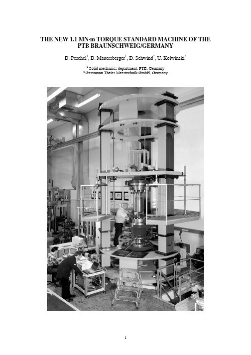
THE NEW 1.1 MN·m TORQUE STANDARD MACHINE OF THE PTB BRAUNSCHWEIG/GERMANYD. Peschel1, D. Mauersberger1, D. Schwind2, U. Kolwinski21 Solid mechanics department, PTB, Germany2 Gassmann Theiss Messtechnik GmbH, GermanyABSTRACTUntil 2003 it was impossible to perform traceable calibrations for torque measuring systems above applied torque values of 200 kN·m anywhere in the world. Up to this figure such calibrations are possible at LNE/Paris. This is despite the fact that a number of applications with considerably larger torque values are known (energy generation, shipbuilding etc.). In addition there are requests for calibrations above the largest measuring range so far available at the PTB (20 kN·m), as realised with a deadweight torque standard machine (20 kN·m TSM) acting on a double-sided lever arm supported in an air bearing.In 2002/2003, a new torque standard machine with a capacity of 1.1 MN·m was constructed and manufactured by GTM Gassmann Theiss Messtechnik GmbH in co-operation with the torque laboratory of the PTB. In 2004, initial evaluations and the analysis of the measurement uncertainty were concluded. First calibrations were already performed in May/June 2004.The machine has a vertical test axis and the effective torque is determined by means of force transducers acting on a double-sided lever arm. Parasitic bending moments and transverse forces, which cannot be entirely avoided, at the locations of the force transducers are measured by strain-gauged bending joints. These disturbances are partly controlled by additional drives and partly electronically processed to correct the measuring signal. This allows to abandon the principle so far applied – i.e. the reduction of parasitic quantities by use of metallic multiple disk couplings which are torsionally stiff and flexible in bending – and to rigidly couple the object to be calibrated. Measurement of the mechanical parasitic quantities during loading and reducing them to a negligible amount with respect to the measurement uncertainty allows the system to be used as national standard with sufficiently small uncertainty of measurement. The aim is to achieve a value of 0.1 % (k = 2) in the measuring range from 5 kN·m to 1100 kN·m.There are further requirements which call for a reduction of the measurement uncertainty in the measurement range up to 100 kN·m which will be dealt with in future.The paper gives an overview of the design, construction and first results of the investigations into the measurement uncertainty.1. INTRODUCTIONMeasurements of torque are required in many different areas of industry, research, safety engineering, technical monitoring, medical technology, handicraft and others. In order to achieve the necessary measuring uncertainty calibrations which are traceable to national standards are required. It is the duty of the national institutes of metrology to provide these standards. However, limits are frequently reached due to the fact that the measuring ranges demanded by industry cannot be covered because of a lack of financial and personnel capacity. Therefore the torque laboratory of the PTB has spent over 10 years on development and procurement of measurement equipment, so that more than 90% of the user requirements could be performed in the past.Frequent enquiries for calibrations at torque levels of 50 kN·m and more as well as 1 N·m and down to a few mN·m resulted in the necessity to complete the torque scale by adding standards for these measuring ranges. A direct loading machine with air-supported lever-mass system and a nominal torque of 1 N·m is at present being commissioned.In 2004 the other end of the torque scale was completed by the installation of a standard machine with a capacity of 220 kN·m in the measuring range 1 and 1100 kN·m in the range 2. The design uses strain controlled elastic hinges [1] for the transmission of force on the measuring lever. This method was developed by GTM and has been used more than 15 times already for force and torque calibration machines, more than half of which are standard machines of national institutes.2 DESIGN OF THE 1.1 MN·m TORQUE STANDARD MACHINETo reach the highest possible accuracy two conditions were invariably considered to be state of the art for torque calibration equipment:• Force generation by acting of discrete load masses in the local gravity field (taking into account air buoyancy) in connection with a lever arm of calibrated length supported in low-friction bearings.• Reduction of the various mechanically disturbing quantities (transverse forces, bending moments) by use of metallic multiple disk couplings which are torsionally stiff and flexible in bending for the mounting of the device under test in the measuring axis [2].Both conditions could not be satisfied in the MN·m measuring range. Force generation by direct mass loading would increase both cost and size of such a machine beyond economic and practical limits. Elastic couplings which can withstand the stresses caused by the desired torque range from 5 kN·m up to 1100 kN·m are difficult to realise in practise and would require different sizes for different capacities and transducer designs, with correspondingly difficult mounting operations.Figure 1: Top of the 1.1 MN·m TSM with force transducer sets acting on the measuring lever arm (computerdesign)Figure 2: Base of the 1.1 MN·m TSM with actuating lever and electrical drives (computer design)The design of the 1.1 MN·m TSM is based on a vertical measuring axis. The machine frame consists of three columns located at 120 degrees around the central test space. At the bottom of the frame is the drive unit, consisting of a double-sided lever arm with two servo-electric spindles. This lever is arranged in a free-floating matter, i.e. the electrical drives and support points are designed as cardanic joints to achieve a statically determined system (no over-constraining) in the operating condition.At the other end of the frame the measuring lever is located. This is also a double-sided arm which resolves the measured torque into a couple of equal forces and transfers them into the frame by means of two multi-component strain controlled hinges. At the same time these forces are measured by the force transducer located between these hinges and the frame.The lower crosshead supports the actuating lever, and the upper crosshead links the columns of the frame. Both are fixed and are clamped to the columns, the latter being of I-section, see Figs.1 and 2. A third movable crosshead carries the double-sided measuring lever. It can be adjusted in height to accommodate test pieces of up to 4 m length. Once set correctly it is also clamped to the three vertical I-beam columns. Both the actuating and the measuring lever carry adapter plates with annularT-grooves of the diameters 500 mm, 700 mm and 900 mm. The corresponding thread size is M36.The established solutions of torque measurement by means of a force couple acting on an unsupported lever all suffer from influences such as deviations of the force direction and unavoidable parasitic components due to elastic deformations at or near the point of load application. A reliable determination of the measuring uncertainty budget was not possible in such cases.The concept of the new torque calibration machine at the PTB permits the generation of the torque with quantifiable measuring uncertainty contributions. Thereby it is possible to achieve a best measurement capability (bmc) for k=2 of 0,1%. In order to arrive at this low bmc value it is essential that the transverse forces and bending moments which are superimposed to the measured forces are known. Fig. 3 shows such a measuring element. It consists of two compression force transducers arranged in series and pre-loaded with 50% of the nominal force. This yields very low remanence effects upon load reversals, since each of the transducers is loaded from 0% to 100% in one direction only (compression) even though the assembly experiences a load reversal from tension to compression due to changing load directions (clockwise or anticlockwise torque). Both force measuring systems onFigure 3: Force-transducer sets for 220 kN·m (small) and 1.1 MN·m (large) and elastic hinge element to measure the parasitic mechanical components in the contact area between force transducer and lever armthe ends of the lever arm are orientated in the same direction. Thus one set is loaded in tension the complementary set is loaded in compression. The main contribution of typical non-linear characteristics of the force transducer sets are compensated in this way. The coupling of the force transducer sets to the measuring lever is made by the multi-component strain controlled hinges. Their strain-gauge bridges provide signals for both bending moments and both transverse forces which are used to generate the control signals for their compensation.The principle of this new machine practically reverses the approach taken by the PTB with respect to parasitic influences: So far the machine designs were based on minimising these effects to negligible amounts by using certain principles of lever support and elastic de-coupling. However, in these designs the actual magnitudes of the effects were not measured during a calibration. The new approach does not rely on minimising the parasitic contributions, but on their accurate measurement and subsequent reduction by adjusting the load levers as well as electronic correction of the readings.During a calibration, an existing or developed parasitic component will be reduced to a negligible amount by moving the actuating lever. Towards this end the actuating lever ismovable in three axes according to the indication of the strain controlled hinges. Three electrical drives are used: With the two main drives the torque is applied and transverse forces at right angle to the longitudinal axis of the measurement lever are eliminated. With the third auxiliary drive transverse forces in the direction of the longitudinal axis of the lever can be minimised. A fourth manual drive supports the actuating lever in the vertical direction, so that the axial force along the measurement axis can be reduced.The auxiliary drive on the actuating lever as well as the two main drives permit to compensate the parasitic components and/or to adjust their symmetry, so that their sum reaches zero. Existing bending moments on the device under test can be minimised by operating both main drives in the same direction: Instead of a torque introduction a side movement results.Flexible couplings in the torque measuring line are no longer necessary. The various disturbances are compensated or at least controlled so as to be symmetric so that their effects are negligible. The applied torque can then be calculated with sufficient accuracy from the measurements of the force couple acting on the lever as measured by the transducer sets.In order to keep the relatively high weight of the measuring lever away from the measuring system and the device under test it is suspended from three wires attached to the movable crosshead. This arrangement is extremely weak in torsion and the existing torque shunt and its small elastic deformations are not relevant for the measurement uncertainty.On the strength of past experiences with the strain controlled hinges in various force and torque standard machines the applied torque of the 1.1 MN·m TSM is calculated from the force couple as measured by the force transducers, taking into account bending moments about the vertical axis as measured by the strain controlled hinges.In parallel with the development of the new standard machine reference torque transducers for the two measuring ranges of the machine have been developed together with HBM, which are based on the type TB2. They are used as an alternative measuring system. The 1100 kN·m reference torque transducer is already in use, and the "small" one for the measuring range 220 kN·m is under development. Due to the design this type is relatively insensitive to various mechanic parasitic components. Using this type of reference system these components must be minimised only with respect to the device under test during the calibration. At the same time the reference measuring system offers the important advantage of being able to monitor the long-term stability between the re-calibrations of the force transducer sets. Continuous monitoring of the measuring system with respect to stability is planned and would thereby give the possibility of introducing flexible re-calibration cycles for the force transducer sets (4 transducer sets in tension and compression force up to 120 kN and 500 kN, respectively).Figure 4: Device under test (700 kN·m) in line with the reference transducer (1.1 MN·m)3. CONDITIONS OF TESTINGExtensive work was necessary for the evaluation and calibration of the force transducer sets.The creep characteristics were determined. With approximately 0.003 % over 30 minutes thecreep is negligible, relative to the best measurement capability of 0.1 %. Non-linearity andhysteresis are to be considered for the interconnection of the two working force transducer sets.The interconnection causes a reduction, by cancellation, of the non-linearity when compared tothat of the single transducers.Remaining parasitic components are minimised to values of about 10 N·m (bending moments)and 50 N (transverse forces) at an applied load of 500000 N·m. From this it is clear that byusing strain controlled hinges better conditions for the device under test are achieved than withmetallic multiple disk couplings which are stiff in torsion and flexible in bending.Figure 5: Typical loading diagram for 200 kN·m stepFig. 5 shows a typical torque-time-diagram with the manual control. Each nominal torque up to1.1 MN·m can be performed within 120 s.With the achieved results of very small parasitic components in connection with the verticalmounting position of the device under test it may be possible in future to reduce the differentmounting adaptations to only one. Corresponding investigations are carried out at present.For a measuring sensor of 700 kN·m capacity the relationship between preparation time and realmeasuring time was determined. Mounting, bolt-up and removal of the measuring sensor tookfour times longer than the actual time required for the pure measurements. In addition duringassembly and disassembly at least two technicians are needed, whereas the calibration itself is aone-man-operation and could be semi-automated in future.4. DIMENSIONS AND TECHNICAL DATAMaximum torque 1,100 kN·mMeasuring range 1: 5 kN·m to 220 kN·mMeasuring range 2: 30 kN·m to 1,100 kN·mBest relative measuring uncertainty (k=2): 0,1% Diameter x height: 4.5 m x 7.3 mMounting space: width x depth x height: 1.2 m x 1.9 m x 4.1 mMaximum permissible weight of the transducers incl. adaptation: 2500 kg5. SUMMARYThe world‘s largest torque standard machine allows calibrations at up to 1.1 MN·m with a measuring uncertainty of 0.1 %. Beyond that calibrations of partial ranges of transducers with extreme capacities can be carried out since the generous mounting space offers ample reserves compared to the dimensions of common transducers. However, the limits of the 1.1 MN·m TSM are reached relatively quickly when actual components are to be mounted since these are often much larger. In these cases the user can only obtain calibrated special reference transducers, corresponding to the main torque range of a national laboratory, which are then used within his own loading devices, and coupled in series with these components. This applies, for example, to drive shafts for ships.The concept of a force introduction without parasitic quantities into a double-sided floating lever on the measuring side as realised here allows a reliable estimation of the uncertainty contributions and will enable to further reduce the currently achieved value of 0.1 % in future. REFERENCES[1] Gassmann, H., Allgeier, T., Kolwinski, U., A new design of torque standard machines, Proceedingsof the 16th IMEKO World Conference, Wien 2000, pp. 40.[2] Peschel, D., Proposal for the design of torque calibration machines using the principle of acomponent system, Proceedings of the 15th IMEKO TC3 International Conference, Madrid 1996, pp. 251-254.Address of the Author:Diedert Peschel, Solid mechanics department, Physikalisch-Technische Bundesanstalt, Bundesallee 100, 38116 Braunschweig, Germany. diedert.peschel@ptb.de。

基于剖面渗透率估算全岩心孔喉半径

第44卷第3期物探化探计算技术Vol.44No.3 2022年5月COMPUTING TECHNIQUES FOR GEOPHYSIC A L AND GEOCHEMIC A L EXPLORATION May2022文章编号：1001-1749(2022)03-0322-07基于剖面渗透率估算全岩心孔喉半径廖万平a b王兴建a b李卿武a,王崇名a,张俊杰a（成都理工大学 a.地球物理学院，b.油气藏地质及开发工程国家重点实验室，成都610059）摘要：岩石孔隙喉道是流体流动的通道，是决定储层储渗性能的关键因素。

为克服传统方法操作复杂、费用高昂、测量周期长且存在安全隐患等因素。

本研究提出一种基于岩心剖面渗透率反距离加权插值法估算全岩心孔喉半径的方法，以油藏岩心和非油藏岩心为实验样品，分别对岩心进行了CT扫描法、扫描电镜法、渗透率插值法求取岩心孔喉半径。

经分析验证，此方法计算出的岩心孔喉半径分布规律与CT扫描法和扫描电镜结果相关性达98%，因此可为全岩心孔喉半径测量提供一种新的方法。

关键词：剖面渗透率；孔喉半径；反距离加权插值法；CT扫描法；扫描电镜法中图分类号：P631.4文献标志码：A DOI：10.3969力.issn.1001-1749.2022.03.070引言在储层评价和油层保护中，岩石孔喉半径是十分重要的参数，应用也很广泛［1—2］。

其主要研究方法大体分为四类：①毛细管压力曲线法；②图像分析法；③三维孔隙结构模拟法；④测井方法等。

然而传统孔喉半径研究的方法存在诸多局限性，毛细管压力曲线法，是通过岩石孔隙的毛细管压力和岩石湿相（或非湿相）饱和度关系曲线定量确定孔喉半径特征［］。

其主要方法有半渗透隔板法、压汞法和离心机法等。

其中半渗透隔板法测试所需时间过长，且半渗透隔板承受压力有限，因此在测低渗岩样时，得到的压力曲线不完整；压汞法虽测定速度快但需要有毒汞做介质，对人体有害，且岩样不能重复使用，加大浪费和成本［4—5］；离心机法所需费用高昂不能满足工业生产需要。

电热耦合

J Comput Electron(2012)11:93–105DOI10.1007/s10825-012-0387-xCoupled electro-thermal simulation of MOSFETs Chunjian Ni·Zlatan Aksamija·Jayathi Y.Murthy·Umberto RavaioliPublished online:31January2012©Springer Science+Business Media LLC2012Abstract Thermal transport in metal-oxide-semiconductor ﬁeld effect transistors(MOSFETs)due to electron-phonon scattering is simulated using phonon generation rates ob-tained from an electron Monte Carlo deviceThe device simulation accounts for a full band descrip-tion of both electrons and phonons considering22types of electron-phonon scattering events.Detailed proﬁles of phonon emission/absorption rates in the physical and mo-mentum spaces are generated and are used in a MOS-FET thermal transport simulation with a recently-developed anisotropic relaxation time model based on the Boltzmann transport equation(BTE).Comparisons with a Fourier con-duction model reveal that the anisotropic heat conduction model predicts higher maximum temperatures because it ac-counts for the bottlenecks in phonon scattering pathways. Heatﬂuxes leaving the boundaries associated with differ-ent phonon polarizations and frequencies are also exam-ined to reveal the main modes responsible for transport.It is found that though the majority of the heat generation is in the optical modes,the heat generated in the acoustic modes C.Ni( )·J.Y.MurthySchool of Mechanical Engineering,Purdue University,West Lafayette,IN47907,USAe-mail:charlesni2006@J.Y.Murthye-mail:jmurthy@Z.AksamijaElectrical and Computer Engineering Department,University of Wisconsin-Madison,Madison,WI53706,USAe-mail:aksamija@U.RavaioliSchool of Electrical and Computer Engineering,University of Illinois,Urbana Champaign,IL61820,USAe-mail:ravaioli@ is not negligible.The modes primarily responsible for the transport of heat are found to be medium-to-high frequency acoustic phonon modes.Keywords Semiconductors·Dielectrics·Phonons·Boltzmann transport equation·Electron Monte Carlo device simulation·Coupled electro-thermal simulation·Micro/nanoscale heat transfer1IntroductionCoupled electro-thermal simulation of sub-micron electron device is of great interest to both academia and industry,due to the fact that self-heating may cause device performance degradation in submicron regime.Sadi et al.[1,2],used a 2-D electron Monte Carlo simulation(MC)coupled with a 2-D solution of the heat diffusion equation(HDE)to study the electrothermal phenomena in Silicon-On-Insulator(SOI) and Silicon-Germanium-on-Insulator(SGOI)metal-oxide ﬁeld-effect transistors(MOSFET).Although they got in-teresting results on device thermal effects and performance degradation,there is a fundamentalﬂaw in their thermal so-lution of the heat diffusion equation,which is well known not valid in submicron regime[3].Raleva,Vasileska et al.[4,5],coupled electron Monte Carlo simulation with the equations for the optical and acoustic energy transfer derived from the phonon Boltzmann Transport Equation(BTE)[6].They used this methodology to study electrothermal effects in the Silicon-On-Insulator (SOI)MOSFET.They showed that the device current de-grades due to heating effects,while pronounced velocity overshoot in the nano-scale device structure(at gate length in the order of20nm)minimizes the current degradation due to lattice heating.Although they solved the equationsFig.1Phonon dispersion for bulk silicon in the X[100]direction. Phonons of the f and g type are marked on the graph[7]for the optical and acoustic energy transfer derived from phonon BTE,their thermal transfer model is a simpliﬁed model which might not be able to capture detailed physics of phonon transport in the submicron devices.To better model thermal transport in submicron devices, it is necessary to correctly resolve the granularity of phonon transport.Figure1shows phonon dispersion curves for sili-con in the[100]direction.Electron-phonon scattering scat-ters energy selectively to high-frequency optical and longi-tudinal phonon modes at the Brillouin zone edge[8–10], which then transfer energy through phonon-phonon scatter-ing processes to other phonon groups.The thermal proﬁle in the MOSFET is thus governed by which phonon groups receive energy from electrons,how fast they scatter to other phonons,and the group velocity of these phonons.If scatter-ing from slow-moving high-frequency optical and acoustic phonons to faster-moving phonon groups is a bottle-neck, high device temperatures would occur;alternatively,if fast-moving phonons are able to move energy quickly to the de-vice boundaries,low device temperatures would result.Cap-turing these detailed physics requires a resolution not only of the electron-phonon scattering rates in both the physical and momentum spaces,but also of phonon scattering and transport mechanisms.A number of published studies have sought to simulate phonon transport at the sub-micron scale. Early studies employed a“gray”description of phonons and employed the Boltzmann transport equation(BTE)in the re-laxation time approximation[3,11].Here,all phonons are grouped into a single mode characterized by a single group velocity and relaxation time.One of the parameters,typi-cally the group velocity,is chosen to reﬂect that of the dom-inant phonon group responsible for transport at the device temperature,such as longitudinal acoustic(LA)phonons;the relaxation time is then computed from the bulk ther-mal conductivity.However,this type of model does not ad-equately capture the large variations in group velocity,spe-ciﬁc heat and scattering rates in MOSFET simulations.Sverdrup[12]and Ju[13]developed and improved a two-ﬂuid or semi-gray BTE model for heat conduction in silicon-on-insulator(SOI)devices.In the two-ﬂuid BTE model,there are two phonon modes:the reservoir mode and the propagation mode.The longitudinal acoustic phonons are lumped into the propagation mode,while the transverse acoustic and optical phonons are lumped into the reservoir mode.Heat generation due to electron-phonon interaction in MOSFET is incorporated into the reservoir mode via a source term,while the heat transport is accomplished by the propagation mode,characterized by a single group velocity. The two modes are coupled by a scattering term character-ized by a single relaxation time,again chosen to match bulk thermal conductivity.The device temperature predicted by this type of model depends strongly on the choice of the group velocity and relaxation time.If the group velocity is picked to be that of a dominant LA group,a too-long relax-ation time between reservoir and propagating modes results, leading to an unrealistically high device temperature.Because of the drawbacks of these approximate models, a number of recent efforts have sought to capture the de-tails of phonon transport,incorporating the details of phonon dispersion,polarization and scattering to different degrees. Narumanchi et al.[14,15]developed a BTE model incorpo-rating phonon dispersion effects to model MOSFET thermal transport.The phonon spectrum was resolved into bands, but only acoustic modes incorporated a ballistic term.The ballistic term was ignored for optical phonons because of their low group velocity,and a single equation for the opti-cal phonon energy was developed.The interactions among the different phonon groups were represented by frequency-dependent relaxation times,which were obtained from the perturbation theory[16].With most of the heat generation assigned to the optical phonon mode,their prediction of the hotspot temperature rise above ambient could be as high as 350%of that predicted by the Fourier diffusion model.This high number was thought to be a result of the zero group velocity assigned to the optical mode.Phonon BTE models incorporating detailed spectral reso-lution require the determination of detailed relaxation times, which can no longer be found simply by matching bulk ther-mal conductivity.Wang[17]developed a new BTE model which directly computes the scattering rate for three-phonon interactions from perturbation theory[16]without making the relaxation time approximation.All modes,including op-tical,are resolved using the BTE with ballistic terms in-cluded.Wang developed a search scheme to determine all three-phonon processes(normal(N)and Umklapp(U))con-tributing to scattering.Field effect transistor(FET)thermalmodeling using this BTE model showed that the optical phonon mode plays an important role in the prediction of the hotspot temperature,since optical phonon velocities are not negligible for intermediate wave-number values.One of the drawbacks of directly computing N and U in-teractions and enforcing conservation rules is that the com-putation of scattering rates becomes very expensive.There are many millions of N and U interactions,which must be evaluated every iteration in a typical computational process. Ni[18]developed an anisotropic relaxation time phonon BTE model based on Ref.[17].This BTE model employs a single-mode relaxation time idea,but the relaxation time is a function of the wave-vector.The model incorporates directional and dispersion behavior and the resulting three-phonon processes satisfy conservation putational expense is allayed by pre-computing single-mode relaxation times,resulting in order-of-magnitude reduction in compu-tational time over Ref.[17].A critical issue in the model development is the accounting for the role of three-phonon N scattering processes.Following Callaway[19],the over-all relaxation rate is modiﬁed to include the shift in the phonon distribution function due to N processes.The relax-ation times so obtained compare reasonably well with those extracted from equilibrium molecular dynamics simulation by Henry and Chen[20].In all the models described above,metal-oxide-semi-conductorﬁeld effect transistor(MOSFET)modeling was undertaken by prescribing an electron-phonon scattering source in the phonon BTE.Typically,a source term is in-cluded in the optical phonon equations,or a prescribed arbi-trary distribution in wave-vector space is used.However,to fully capture the granularity of thermal transport,it is nec-essary to describe phonon generation as a function of both phonon mode and frequency.Monte Carlo simulation has long been used to model electron transport in semiconduc-tor devices[21].Pop et al.[8–10]developed a Monte Carlo simulation(e-MC)scheme to calculate Joule heating in sili-con.In their scheme,they used analytic,non-parabolic elec-tron energy bands to model electron transport,while using an isotropic,analytic phonon dispersion model for electron-phonon scattering,distinguishing optical/acoustic and lon-gitudinal/transverse phonon branches.Their Monte Carlo simulation was used to examine the details of the phonon generation spectrum by electron-phonon interaction in sili-con.They found that a signiﬁcant portion of the generated phonons were optical phonons or acoustic phonons near the Brillouin zone edge.Their simulations did not focus on the details on phonon transport,however.Sinha et al.[22]developed a split-ﬂux form of the non-equilibrium phonon BTE model in which the phonon generation spectrum was taken from Monte Carlo simula-tion of electron-phonon scattering.They split the phonon departure-from-equilibrium function into two components:one that traces the evolution of the emitted phonons before they thermalize through scattering,and another that traces the diffusion of the thermalized phonons.The former was obtained by solving the ballistic BTE in a spatial region of the order of a mean free path.The thermalized component was assumed to correspond to the solution of the BTE in the limit of diffusive transport.Rowlette and Goodson[23]coupled the electron Monte Carlo(e-MC)model of Refs.[8–10]with the split-ﬂux model for phonon transport to perform a self-consistent sim-ulation of non-equilibrium transport in MOSFETs.Their coupled simulation begins with an isothermal e-MC simu-lation solved self-consistently with the Poisson equation in the device.The net phonon-generation rates as a function of position and phonon frequency are gathered and fed into the split-ﬂux phonon transport model,whose solution leads to an updated distribution of phonons as a function of position. The effective temperatures for the dominant optical f-and g-type phonons as well as for the LA and TA branches are then computed and passed back to the e-MC to adjust the electron-phonon scattering rates.They used this fully cou-pled electron-phonon model to study a1-D n+/n/n+sili-con device and found that near the hotspot the temperature is anomalously high,possibly as a result of ballistic trans-port.The e-MC solver developed by Pop et al.[8–10]as-sumes analytical,non-parabolic electron energy bands and analytic phonon dispersion curves.Recently,Aksamija[7] improved an existing full-band Monte Carlo simulation tool developed at University of Illinois at Urbana-Champaign [24]to provide phonon generation terms due to electron-phonon scattering.He employed a full-band description of electrons and phonons.The electron band structure was cal-culated using the empirical pseudo-potential model of Co-hen and Bergstresser[25].The electron scattering mecha-nisms considered in Monte Carlo simulation included intra-valley acoustic phonon scattering,X–X f and g type inter-valley phonon scattering,and X–L inter-valley phonon scat-tering.The Monte Carlo simulation was performed self-consistently with a solution of the Poisson equation to up-date the electricﬁeld during the simulation.The e-MC sim-ulation may be used to provide phonon generation rates to a phonon BTE simulation to accurately predict sub-micron thermal transport in MOSFETs.The goal of this paper is to couple the anisotropic re-laxation time phonon BTE simulation to a computation of the phonon generation spectrum calculated using the Monte Carlo simulator of Ref.[7].The Monte Carlo simulation[7] provides the phonon generation spectrum at different spa-tial positions and different positions in momentum space. The phonon generation spectrum so obtained is incorpo-rated in the anisotropic relaxation time phonon BTE model of Ref.[18]to predict more realistically the location andtemperature of a hotspot in the MOSFET device.The ap-proach taken in this paper not only improves the representa-tion of the electron-phonon scattering source to the phonon ﬁeld,but also resolves the details of phonon transport more completely than in previous studies.However,only one-way coupling is considered in that the predicted temperature ﬁeld does not affect electron-phonon scattering.Thus the electron mobility is not affected by the device self-heating and the drain current reduction due to self-heating is not captured.The device Monte Carlo simulation was done at ﬁxed tem-perature of 300K.The model is applied to the prediction of the temperature ﬁeld in a MOSFET and the detailed path-ways for energy transport are identiﬁed and discussed.2Phonon dispersion for siliconBulk silicon has six phonon dispersion branches:two trans-verse acoustic phonon branches (TA1and TA2),one longi-tudinal acoustic phonon branch (LA),two transverse opti-cal branches (TO1and TO2)and one longitudinal optical branch (LO).The dispersion curves for silicon used in this paper are calculated using the adiabatic bond charge model [26].A fully anisotropic Brillouin zone is taken into ac-count.3Anisotropic relaxation time modelA complete description of the anisotropic relaxation time model may be found in Ref.[18];a brief summary is given below.The phonon BTE in the energy form [18]under the single mode relaxation time assumption may be written as:∂e (r ,K ,t)∂t +∇·(e (r ,K ,t)v g )=(e 0−e(r ,K ,t))1τ3phonon +1τI +1τB+q vol (r ,K )(1a)with e (r ,K ,t)=lim3K →01(2π)1K3KωN(r ,K ,t)d 3K(1b)ande 0=lim3K →01(2π)313K3Kωexp ( ω/k B T lattice )−1d 3K(1c)Here q vol (r,K)is the volumetric heat generation term due to electron-phonon scattering.N(r ,K ,t)is the phonon oc-cupation number,and e (r ,K ,t)is the phonon energy den-sity for phonons of wave vector K at position r and time t .It denotes the phonon energy per unit physical volume per unit K-space volume at (r ,K ,t).e 0(ω)is the phonon en-ergy density corresponding to the Bose-Einstein distribution function evaluated at the lattice temperature T lattice .v g (K )is the phonon group velocity corresponding to the wave vec-tor K .It may be calculated from the phonon dispersion by v g =∇K ω(2)The adiabatic bond charge model [26]is used to com-pute the dispersion relation,as described in Ref.[18].The effective relaxation time τ(K )depends on the wave vector;a dependence on polarization is implied throughout.It con-tains the inﬂuence of three-phonon scattering,represented by a relaxation time τ3phonon and isotope scattering,repre-sented by τI ;Matthiesen’s rule [17]is applied to compute their combined inﬂuence.Boundary conditions on (1a )include the speciﬁcation of thermalizing boundaries,specular boundaries or partially specular/partially diffuse boundaries.Boundary scattering is computed by representing the appropriate boundaries of the MOSFET domain as either partially or fully diffusely re-ﬂecting.A detailed description of the treatment of boundary conditions may be found in Ref.[18].4Numerical methodEquation (1a )is discretized using the ﬁnite volume method and solved numerically.The phonon energy distribution function e (r ,K ,t)is discretized in both the spatial and wave vector domains.The spatial domain is discretized into control volumes or cells.The three-dimensional wave vec-tor space is discretized using spherical coordinates and con-sists of an angular space of 4πand a wave number space [0,K zone ],where K zone is the maximum K value in each di-rection,accounting for the shape of ﬁrst Brillouin zone [18].The angular space is discretized into N θ×N φcontrol an-gles,each of extent of i ,corresponding to direction i ;θand φare the polar and azimuthal angles.The wave num-ber space is discretized into N k bands,each of extent K j ,corresponding to band j .Each polarization is discretized inthis way.The discrete energy density e ijcorresponding to direction i and band j is stored at the cell centroids.The phonon BTE is integrated over the control volume,control angle and wave number band for each polarization,resulting in an energy balance for each spatial control vol-ume for direction i ,wave number band j and polarization.A third-order SMART scheme [27]is used to discretize the convective operators.A second-order discretization of the scattering terms is used.The phonon energy densities are solved sequentially and iteratively,cycling through each di-rection and band in turn.For each direction and band,the discrete equation set is solved using the line-by-line tri-diagonal matrix algorithm (TDMA).5Lattice temperatureOnce the discrete energy density at the cell centroids is computed,the lattice temperature is determined.In order to guarantee energy conservation,the summation of the source terms on the right hand side of (1a )over all directions and bands should be zero,if q vol (r ,K )=0.The following equa-tion must be satisﬁed:(e 0−e (r ,K ,t)) 1τ3phonon +1τI +1τB d 3K =0(3)The lattice temperature,T lattice ,is deﬁned so that (3)is sat-isﬁed,using the deﬁnition of e 0given in (1c ).6Phonon relaxation timesA key feature of the anisotropic relaxation time model is thedevelopment of single-mode relaxation rates based on a rig-orous computation of three-phonon interactions.Klemens et al.[16]developed three-phonon interaction rates based on perturbation theory.Based on these rates,Wang [17]de-veloped a full-scattering phonon BTE model which directly computes three-phonon scattering rates for N and U pro-cesses.Details may be found in Ref.[18];a brief overview is given here for completeness.Three-phonon interactions must satisfy energy and mo-mentum conservation rules,given by [16]ω+ω ↔ω (4)K +K ↔KN processesK +K ↔K +bU Processes(5)Here,ω,ω ,ω are three interacting phonons with corre-sponding wave vectors K ,K ,K ,and b is the recipro-cal lattice vector.Wang [17]developed a search techniqueto identify all possible three-phonon normal (N)and Umk-lapp (U)processes between interacting phonons.The pro-cess employs a discretization of the Brillouin zone in the manner described in this paper,and triads of interacting phonons (ij),(kl)and (mn)satisfying (4)and (5)are found.Here (i,j)denotes the direction i and wave number band j of an interacting phonon;(kl)and (mn)are interpreted in a similar fashion.Consideration of polarization in determin-ing these triads is implied.Given a such a triad,the scattering rate may be cal-culated from the perturbation theory derived by Klemens and co-workers [16,28].For an interaction of the type K +K ⇔K ,the scattering rate due to three-phonon pro-cesses is given by: dN dt 3-phonon = K2|C 3|2M ωω ωπδt (ω+ω −ω )×(NN (N +1)−(N +1)(N +1)N )(6)Here |C 3|2=(4γ23G )(M 22)(ωω ω )2,γis the Gruneisen con-stant,G is the number of atoms per unit cell,v is thesound velocity,and M is the atomic mass.N is the oc-cupation number of mode K ,while N and N are those corresponding to K and K .The summation is over all possible interactions undergone by a phonon of wave vec-tor K .The anisotropic relaxation time model employs a single-mode relaxation time approximation which signif-icantly cuts down on solution time while preserving the granularity of phonon-phonon interaction bottlenecks.Un-der this approximation,the three-phonon relaxation time τ3phonon in (1a )is computed by assuming that the only non-zero departure from equilibrium occur for the phonon mode K ,i.e.,the phonon mode for which the BTE is be-ing solved;the departure from equilibrium of phonons with wave vectors K and K are set to zero.Under this approx-imation,it is possible to show that for a single three-phonon interaction for phonon K ,the single mode relaxation time may be written as1τ3phonon (K )=2|C 3|2M ωω ωπδt (ω+ω −ω )(N 0−N0)(7)Details may be found in Ref.[18].The computational savings afforded by the anisotropic relaxation time model now become evident.To evaluate the scattering rate in (6),the non-equilibrium distribution func-tions N,N and N are necessary.These change iteration-to-iteration in a typical computational procedure.Since there may be many millions of N and U interactions,the scattering term update becomes computationally very ex-pensive even for coarse spatial meshes.On the other hand,τ3phonon in (7)depends only on the equilibrium distributions of the interacting phonons,and may be computed a priori and stored,greatly reducing the cost per iteration.In the present implementation,a list of all permitted three-phonon N and U processes is ﬁrst determined using the procedure described in Wang [17].Based on these per-mitted interactions,a single-mode relaxation time as a func-tion of discrete wave vector,polarization and temperature is computed and stored in a look-up table.Interpolations within this look-up table are used to compute the distribu-tions of relaxation time in physical and wave-number space in the MOSFET simulation.Incorporation of N processes is performed through the use of a shifted equilibrium distribu-tion,as described by Callaway [19].Details of the relaxation time computations as well as validation against experimen-tal measurements may be found in Ni [18].7Monte Carlo simulation including full phonon dispersionJoule heating or phonon generation in the device due to electron-phonon interaction may be obtained from Monte Carlo simulation.A three-dimensional ensemble Monte Carlo simulator with a self-consistent non-linear Poisson solver[29]is employed here;a quantum correction based on theﬁrst moment of the Wigner equation is used[7].The Monte Carlo simulator accounts for a full band structure for electrons which was implemented in[30].The6X valleys of the lowest electron conduction band at(±0.85×2π/a,0,0),(0,±0.85×2π/a,0),and (0,0,±0.85×2π/a)in the wave vector space(a is the lat-tice constant of bulk silicon[7]),and the next higher L val-leys in the conduction band,are considered.The transitions may be categorized into the following types:intra-valley transitions(within one X valley),inter-valley X–X f type transitions(between a valley and any of the four valleys closest to it),inter-valley X–X g type transitions(between a valley and its opposite valley),and inter-valley X–L transi-tions.Figure1shows the f and g type transitions graphically.A g-type transition,for example,involving electrons go-ing from(0.85×2π/a,0,0)to(−0.85×2π/a,0,0)would cause a phonon at(1.7×2π/a,0,0)to be generated.In the irreducible wedge of theﬁrst Brillouin zone,the correspond-ing K value would be(0.3×2π/a,0,0)[7].All the other g type transitions may be obtained exploiting the symmetry of the lattice.The energies of the phonons involved in each transition may be tabulated and used to simplify the scattering rate calculation in the Monte Carlo simulation.As mentioned above,four types of transitions,i.e.,intra-valley,X–X f type, X–X g type,and X–L inter-valley transitions,are consid-ered.For each type of transition,there are several phonon branches on which phonons may be emitted or absorbed.A total of22different kinds of scattering events resulting from these interactions are shown in Table1.The transition rates or probabilities are tabulated for these22scattering events in the Monte Carlo simulator.The scattering prob-abilities are also tabulated in the Monte Carlo simulator by the energy of the electron involved in the events listed in Ta-ble1.They are calculated by analytically integrating Fermi’s Golden Rule over all initial electron momenta k with a given energy and all the possibleﬁnal momenta k [7].Whenever a collision,resulting in either emission or ab-sorption,occurs,an average phonon energy corresponding to the chosen event type is either subtracted(for emission)or added(for absorption)to the current electron energy.These energies are listed in Table1.Theﬁnal energy of the elec-tron is then used to look up theﬁnal state of the electron after collision in a table of electron momenta sorted by energy in the irreducible wedge of theﬁrst Brillouin zone.Then the Table1Classiﬁcation of scattering events[7]Event Valley Sign Branch EnergyE avg(meV)1Acoustic Absorption TA/LA0to45meV 2Intra-valley Emission TA/LA0to45meV 3Absorption TA18.95824LA/LO47.39545X–X f TO59.02886TA12.06437LA18.52738X–X g TO/LO62.04499X–X f Emission TA18.958210LA/LO47.395411TO59.028812X–X g TA12.064313LA18.527314LO/TO62.044915X–L Absorption TO57.908516LO54.634017LA41.363218TA16.976219X–L Emission TO57.908520LO54.634021LA41.363222TA16.9762 actualﬁnal state in the complete3-D momentum space is chosen randomly by symmetry considerations,according to the speciﬁc type of scattering that occurred[31].For exam-ple,for X–X f type scattering,the largest component of the momentum in theﬁnal state must be made perpendicular to the largest component of the momentum in the initial state, while other types of scattering may have their signs and or-dering chosen at random[7].A full phonon dispersion relation,calculated from the adiabatic bond charge model[26]and tabulated for look-up, is included to ensure accuracy.An iterative algorithm intro-duced by Pop et al.[8]is adapted to ensure that all scatter-ing events conserve energy and momentum with the use of the full phonon dispersion relationship.As shown in Fig.2, this algorithm starts at each scattering event with an estimate of the phonon energy,E est,involved.This estimated energy is taken from those listed in Table1(E est=E avg).From the resulting electron energy E(k )=E(k)±E avg,theﬁnalstate k is looked up,and the phonon momentum K is de-termined by K=k±k .Its corresponding phonon energy E(K)is determined from the full phonon dispersion rela-tion and used as the next guess of the electronﬁnal energy E(k )=E(k)±E(K).Theﬁnal state k is again looked up and the procedure described above repeated until aﬁ-nal state satisfying both momentum and energy conserva-。

finFET

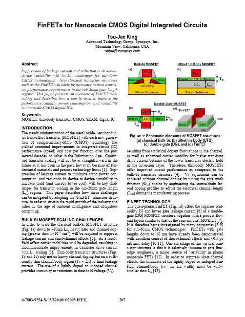
Optimization of Fin Orientation The transconductance of a FinFET is dependent on its layout orientation, due to carrier mobility anisotropy in crystalline Si [8]. The channel surfaces of a FinFET lie in the (110) crystallographic plane when the fin is oriented parallel or perpendicular to the wafer flat or notch of a standard (100) wafer. Hole mobility is enhanced, while electron mobility is degraded, for a (110) Si surface as compared with a (100) Si surface [15]. To simultaneously achieve maximum NMOS and PMOS drive currents, a (100) sidewall surface for NMOS and (110) sidewall surface for PMOS is desirable. This can be achieved by orienting the PMOS fins to be either perpendicular or parallel to the flat or notch of a (100) wafer and orienting the NMOS fins to be rotated at a 45o angle (Fig. 3). Non-Manhattan layout geometry may pose a yield issue for sub-wavelength lithography, however. An alternative approach is to use a (110) wafer to allow the optimal CMOS FinFET sidewall surface orientations to be achieved with Manhattan layouts.

在LS-Prepost 建立sph模型的详细过程

LS_Prepost关键操作1.模型建立立方体模型Part编号起始节点号：粒子密度圆柱体模型圆台/坐标2.坐标数据库IFOR M Outp utform果设置为3，单元有一个综合点，则三个结果将相同。

如果值超过3，则在单元中的第一个MAXINT 综合点将会被输出。

注意：如果单元拥有一系列综合点，而MAXINT 没有被设置成3，则你将无法获得中间表面结果值，详见下面的附注。

STRFLG Setto1todumpstraintensorsforsolid,shellandthickshellelementsforplottingbyLS-PREPOSTandA SCIIfileELOUT.Forshellandthickshellelementstwotensorsarewritten,oneattheinnermostandoneattheouter mostintegrationpoint.Forsolidelementsasinglestraintensoriswritten. SIGFLG FlagforincludingstresstensorintheshellLS-DYNAdatabase:EQ.1:include(default), EQ.2:exclude.EPSFLG FlagforincludingtheeffectiveplasticstrainsintheshellLS-DYNAdatabase:EQ.1:include(default),制结果EQ.2:exclude.RLTFLG FlagforincludingstressresultantsintheshellLS-DYNAdatabase:EQ.1:include(default),EQ.2:exclude.ENGFLG FlagforincludingshellinternalenergydensityandthicknessintheLSDYNAdatabase: EQ.1:include(default),EQ.2:exclude.CMPFLG Orthotropicandanisotropicmaterialstressandstrainoutputinlocalmaterialcoordinatesystemforsoli ds,shellsandthickshells.EQ.0:global,EQ.1:local.IEVERP Everyplotstatefor“d3plot”databaseiswrittentoa separatefile.Thisoptionwilllimitthedatabaseto1000states:BEAMIPmulation.DCOMPse.abase.SHGESTSSZN3THDTEQ.1:on(default)NINTSLD NumberofsolidelementintegrationpointswrittentotheLS-DYNAdatabase.Thedefaultvalueis1.Fo rsolidswithmultipleintegrationpointsNINTSLDmaybesetto8.Currently,noothervaluesforNINTSLDareallo wed.Forsolidswithmultipleintegrationpoints,anaveragevalueisoutputifNINTSLDissetto1.PKP_SEN Flagtooutputthepeakpressureandsurfaceenergycomputedbyeachcontactinterfaceintotheinterface forcedatabase.Toobtainthesurfaceenergy,FRCENG,mustbesentto1onthecontrolcontactcard.WhenPKP_SE N=1,itispossibletoidentifytheenergiesgeneratedontheupperandlowershellsurfaces,whichisimportantinmetal formingappli-cations.ThisdataismappedaftereachH-adaptiveremeshing.EQ.0:NodataiswrittenEQ.1:OutputthepeakpressuresandsurfaceenergybycontactinterfaceSCLP Ascalingparameterusedinthecomputationofthepeakpressure.Thisparameterisgenerallysettounity(thedefault),butitmustbegreaterthan0.MSSCL OutputnodalinformationrelatedtomassscalingintotheD3PLOTdatabase.Thisoptioncanbeactivatedi fandonlyifDT2MS<0.0,seecontrolcard*CONTROL_TIMESTEP.Thisoptionisavailablestartingwiththeseco ndreleaseofVersion971.EQ.0:NodataiswrittenEQ.1:OutputincrementalnodalmassEQ.2:OutputpercentageincreaseinnodalmassTHERM Outputofthermaldatatod3plot.Theuseofthisoption(THERM>0)maymakethedatabaseincompatible withother3rd partysoftware.EQ.0:(default)outputtemperatureEQ.1:outputtemperatureEQ.2:outputtemperatureandfluxdedtotheD3PLOTorD3PARTdatabasewheretheyaredisplayedasbeamelements(similartooption0).Inthisopti ontheelementresultantforceiswrittentoitsfirstdatabasepositionallowingbeamaxialforcesandspringresultantf orcestobeplottedatthesametime.Thiscanbeusefulduringsomepost-processingapplications.NPLTC DT=ENDTIME/NPLTCappliestoD3PLOTandD3PARTonly.ThisoverridestheDTspecifiedinthefir stfield.PSETID SET_PARTIDforD3PARTonly.IOOPT ThisoptionappliestotheD3PLOTfileonly.Flagtogovernbehavioroftheplotfre-quencyloadcurvedefin edbyLCDT:EQ.1:Atthetimeeachplotisgenerated,theloadcurvevalueisaddedtothecurrenttimetodeterminethenextp lottime(thisisthedefaultbehavior).EQ.2:Atthetimeeachplotisgenerated,thenextplottimeTiscomputedsothatT=thecurrenttimeplustheloa步长dcurvevalueattimeT.EQ.3:Aplotisgeneratedforeachabscissapointintheloadcurvedefinition.Theactualvalueoftheloadcurvei signored*CONTROL_SPHNCBS Numberofcyclesbetweenparticlesorting粒子分类搜索循环次数BOXID SPHapproximationsarecomputedinsideaspecifiedBOX.WhenaparticlehasgoneoutsidetheBOX,itis deactivated.Thiswillsavecomputationaltimebyeliminatingparticlesthatnolongerinteractwiththestructure. 指定BOX内的SPH粒子参与计算。

Calculation of transverse hydrodynamic coefficients using computational fluid dynamic approach

Technical noteCalculation of transverse hydrodynamic coefﬁcients using computationalﬂuid dynamic approachAmit Tyagi*,Debabrata SenDepartment of Ocean Engineering and Naval Architecture,Indian Institute of Technology,Kharagpur-721302,West Bengal,IndiaReceived23November2004;accepted30June2005Available online7October2005AbstractComputational Fluid Dynamic(CFD)based on Reynolds Averaged Navier–Stokes equation is used for determining the transverse hydrodynamic damping force and moment coefﬁcients that are needed in the maneuverability study of marine putations are performed for two geometrical shapes representing typical AUVs presently in use.Results are compared with available data on similar geometries and from some of the available semi-empirical relations.It is found that the CFD predictions compares reasonable well with these results.In particular,the CFD predictions of forces and moments are found to be nonlinear with respect to the transverse velocity,and therefore both linear and nonlinear coefﬁcients can be derived.A discussion on the sources of the component forces reveal that the total force and moment variations should in fact be nonlinear.q2005Elsevier Ltd.All rights reserved.Keywords:CFD;Linear coefﬁcient;Non-linear coefﬁcient;Sway force;Yaw moment1.IntroductionApplication of computationalﬂuid dynamic(CFD)to the maritime industry continues to grow as this advanced technology takes advantage of the increasing speed of computers. Numerical approaches have evolved to a level of accuracy,which allows them to be applied for practical ship resistance and propulsion computations by industry.In the recent *Corresponding author.Tel.:C919434138579;fax:C913222255303.E-mail address:amittyagi1979@(A.Tyagi).past,CFD is also being applied to determine some of the hydrodynamic coefﬁcients that are needed in evaluating maneuvering characteristics of marine vehicles.The hydrodynamic forces and moments on the body results from the distribution of pressure(p)and shear stress(t)over the surface.The resulting force R can be resolved into lift(L)and drag(D)forces perpendicular and parallel to the velocity,respectively.The longitudinal force X along the longitudinal axis and the transverse force Y normal to the longitudinal axis of the body are related to L and D as follows:X0Z C D cos a K C L sin a;Y0Z C D sin a C C L cos a(1) where X0,Y0,C D(drag coefﬁcient)and C L(lift coefﬁcient)are the non-dimensional form of X,Y,D and L,respectively,non-dimensionalisation byð1=2Þr L2V2.a here is angle of attack deﬁned as the angle between velocity and longitudinal axis of the body.The transverse force Y can then be determined once C D and C L are known.Computation of C D and C L can be performed in several ways.For attachedﬂow, pressure can be determined using inviscidﬂow theory.Skin friction in a viscousﬂuid can be determined from a boundary layer solution coupled with inviscidﬂow solution. However,boundary layer solution is not suitable whenﬂow separates,since the solution tend to“blow up”in the region ofﬂow separation.For the separatedﬂow,therefore,the complete solution is achieved by Navier–Stokes equation.The main objective of the present work is to determine the transverse velocity dependent force and moment coefﬁcients using Reynolds Averaged Navier–Stokes (RANS)solver.This is equivalent to determining variation of Y0and N0against a,where N0is the non-dimensional moment about some reference point on the body.Majority of the available empirical relation provide only the linear damping coefﬁcients,which are presumed to hold good for small value of a.However,the present computations show that the nature of these forces and moments are essentially nonlinear and therefore for adequate representation for these forces and moments a linear model is insufﬁcient even over a small-velocity range.To gain conﬁdence in CFD computed results,comparison with available data in literature based on computation and semi-empirical formulae for geometries of comparable shapes are also reproduced and results are discussed in detail.putational detailsTwo geometries have been used in this study.Theﬁrst model is axisymmetric with diameter D,a hemispherical nose and a sinusoidal stern with tail radius0.1D.The stern proﬁle is generated using the relation:r R Z sin q Z sinp x2L R(2)where,L R is the length of the rear section over which the stern is tapered,R Z D/2,x is the longitudinal coordinate measured from the aft perpendicular and r is radius of the stern section.This shape and proﬁle,ﬁrst used by Kempf(White,1977),is preferred over a pointed tail since most AUV shapes have aﬁnite diameter tail sectionA.Tyagi,D.Sen/Ocean Engineering33(2006)798–809799The second model has the same proﬁle but with an elliptic cross-section of major and minor axis 2b and 2c Z D,respectively.These two geometries are referred as Kempf model and BlueEyes model in the sequel.Figs.1–3show a schematic plot of the two geometries and stern shape.Computations for C D ,C L and C M are performed for both the geometries over a range of angle of attack a in deeply submerged condition using the commercially available CFD solver FLUENT.This code solves the Reynolds Averaged Navier–Stokes equation based on SIMPLAC (Ferziger and Peric,2002)algorithm using ﬁnite volume method.The realizable k K 3model (Shih et al.,1995),with an enhanced wall treatment,is used for modelling the Reynolds stresses.The length L of the vehicle is 1.5m with L R Z 2.5D and computations are performed at velocity V Z 2m/s (these numbers are typical to AUV’s).Using Eq.(1)the non dimensional transverse force Y 0can be calculated from the computed values of drag and lift coefﬁcients at various angles of attack.Note that the non-dimensional moment N 0is same as C M (all computation are performed with the body in horizontal plane XY ;the transverse force Y 0and moment N 0are then the sway force and yaw moment,respectively).To determine the hydrodynamic coefﬁcients for the computed force and moment,the following quadratic models are used:Y 0Z Y 0v ,v 0C Y 0vv ,v 0j v 0j(3)N 0Z N 0v ,v 0C N 0vv ,v 0j v 0j (4)where,v 0Z sin a .Unlike in many applications,no approximation related to the smallness of the angle of attack is used,therefore v 0can be reasonably large.By using appropriate curve-ﬁtting to the computed data,the coefﬁcients ðY 0v ;Y 0vv ;N 0v ;N 0vv Þcan easily be determined.Successful computations of turbulent ﬂows require some consideration during the mesh generation.Since turbulence (through the spatially varying effective viscosity)plays a dominant role in the transport of mean momentum and other parameters,one must ascertain that turbulence quantities in complex turbulent ﬂows are properly resolved if high accuracy is required.Due to the strong interaction of the mean ﬂow andturbulence,Fig.1.Proﬁle and midship section of KempfModel.Fig.2.Proﬁle and midship section of BlueEyes Model.A.Tyagi,D.Sen /Ocean Engineering 33(2006)798–809800the numerical results for turbulent ﬂows tend to be more susceptible to grid dependency than those for laminar ﬂows.To resolve the regions where the mean ﬂow changes rapidly and there are shear layers with a large mean rate of strain,one must generate sufﬁciently ﬁne mesh.Three of the parameters characterizing a computational grid are total number of grid points,location of outer computational boundaries,and minimum spacing (initial spacing normal to body surface).The minimum spacing is generally based on y C ,a dimensionless parameter representing a local Reynold’s number in the near-wall region.This parameter is deﬁned as (Schlichting,1966)y C Z yu Ãn (5)where,y Z distance from the wall surface,u ÃZ ﬃﬃﬃﬃﬃﬃﬃﬃﬃt w =r p ,t w Z shear stress at the wall,r Z density and n Z kinematic viscosity.Using ﬂat-plate boundary layer theory,this parameter can be derived asy C Z 0:172y LRe 0:9(6)where,Re Z Reynold’s number based on body length.An estimate of the minimum grid spacing can be determined by setting y C Z 1and solving for the value of y /L using Eq.(6).It should be noted here that the y C value from Eq.(5)is based on a turbulent boundary layer on a ﬂat plate.Therefore,it is used only as an estimate in cases where the geometry is not actually a ﬂat plate.The real y C is not constant but varies over the wall surface according to the ﬂow in the boundary layer.While no systematic grid-sensitivity study is reported here,computations are performed using sufﬁciently ﬁne structured mesh.A schematic of this arrangement is shown in Fig.4.Fig.4.Schematic of grid structured around the body (not to scale).A.Tyagi,D.Sen /Ocean Engineering 33(2006)798–8098013.Results and discussionThe variation of the force and moment against transverse velocity computed for the Kempf geometries with L /D Z 10(K1)&L /D Z 6(K2)and the BlueEyes (BE)geometry are displayed in Figs.5and 6.In order to have conﬁdence on the present CFD results,it is necessary to compare these values with available results.Unfortunately,available data on hydrodynamic coefﬁcients for submerged vehicles is extremely scarce in literature.Therefore,a direct comparison of the computed derivatives with available results is difﬁcult.As such,since even for same geometry,the coefﬁcient values obtained from different sources show large scatter (Roderick,1993),it can only be said that the estimated coefﬁcient values presently are at best accurate within some bound.Since the main objective of the present work is to show that the CFD results are within the acceptable range and more importantly to show that CFD results essentially predict the forces/moments as nonlinear variation of the velocity,comparison is made with the limited available results on axisymmetric bodies as well as with data determined from available semi-empirical regression based relations.Two of such relations used here are one given by Clarke based on a combination of slender body theory and regression analysis of ship data and the low aspect ratio wing theory of Jones,both of them are given in (Lewis,1989).Both these relations were developed for ship hull shapes.However,for comparable values of breadth-draft ratios,it is assumed here that these may also be applied within reasonable accuracy for submerged hulls.This is not unreasonable,since for a slow moving surface-piercing vehicle for which the free-surface effects are negligible,the ﬂow over a hull can be approximated within reasonable accuracy by a double hull in inﬁnite ﬂuid.In the present work,the CFD results are for a slow moving AUV-type conﬁguration and therefore comparison of results from these relations are expected to be at least indicative of the range and trend.A description of the different sources and the associated symbols is given in Table 1while Table 2shows the numerical values of the results from these differentsources.Fig.5.Non-dimensional transverse (sway)force for zero yaw rate.A.Tyagi,D.Sen /Ocean Engineering 33(2006)798–809802The transverse forces and moments can in general be divided in two parts:an inviscid (potential ﬂow)part,and a part arising from viscous or real ﬂuid effects.At small angle of attack,there is no boundary layer separation,and the ﬂow remains attached.In this situation,the body essentially behaves like a lifting surface and the forces/moments canbe Fig.6.Non-dimensional transverse (yaw)moment for zero yaw rate.Table 1SourcesSymbolsDescription K1Present computation using FLUENT for Kempf model with L /D Z 10K2Present computation using FLUENT for Kempf model with L /D Z 6BEPresent computation using FLUENT for BlueEyes model with 2b /c Z 2.8and L /2c Z 6A1Existing CFD results for an axixymmetric body of revolution (6degree polynomial (Lin et al.,2004))with L /D Z 10A2Existing CFD results for an axixymmetric body of revolution (6degree polynomial (Lin et al.,2004))with L /D Z 4SubExperimental results for a submarine (Sen,2000)EO1Experimental results for ESSO OSAKA model (Hydronautics Inc.(Post Test)(Roderick,1993))EO1AExperimental results for ESSO OSAKA model (Hydronautics Inc.(Pre-Test)(Roderick,1993))C(K1)Computation using empirical relation based on Clarke regression (Lewis,1989)for Kempf model with L /D Z 10(T Z D /2)C(K2)Computation using empirical relation based on Clarke regression (Lewis,1989)for Kempf model with L /D Z 6(T Z D /2)C(BE)Computation using empirical relation based on Clarke regression (Lewis,1989)for BlueEyes model with 2b /c Z 2.8L /2c Z 6(T Z c )WT(K1)Computation using empirical relation based on Jones low aspect ratio wing theory (Lewis,1989)for Kempf model with L /D Z 10(T Z D /2)WT(K2)Computation using empirical relation based on Jones low aspect ratio wing theory (Lewis,1989)for Kempf model with L /D Z 6(T Z D /2)WT(BE)Computation using empirical relation based on Jones low aspect ratio wing theory (Lewis,1989)for BlueEyes model with 2b /c Z 2.8and L /2c Z 6(T Z c )A.Tyagi,D.Sen /Ocean Engineering 33(2006)798–809803determined from inviscid ﬂow theory.These potential ﬂow forces have a linear relation with angle of attack.Thus it may be stated that the linear coefﬁcients Y 0v and N 0v in (3)and(4)represent the force/moments arising from the inviscid part of the ﬂow.At large angles of attack,however,there exists a cross-ﬂow separation which has a nonlinear relation with angle of attack.(This nonlinearity may be approximated by quadratic or cubic variation with angle of attack.)Therefore the nonlinear part of the forces/moments in (3)and (4),i.e.Y 0vv ,v j v j and N 0vv ,v j v j can be considered as forces/moments due to viscous effect of the ﬂow,which becomes increasingly important as the angle of attack increases.This therefore suggests that the total force,having a linear and nonlinear component as given by Table 2Transverse hydrodynamic coefﬁcientsSourceY 0v Y 0vv N 0v N 0vv K10.00730.03630.0102K 0.0031K20.00940.07670.0284K 0.0185BE0.01090.04540.0271K 0.0136A10.00210.0519A20.01480.1045Sub0.04560.07360.0138K 0.0199EO10.02050.03380.00790.0000EO1A0.01570.05800.0092K 0.0034C(K1)0.01070.0049C(K2)0.02760.0153C(BE)0.03790.0153WT(K1)0.00780.0039WT(K2)0.02180.0109WT(BE)0.02180.0109Fig.7.Linear component of non-dimensional transverse (sway)force for zero yaw rate:comparison with existing data.A.Tyagi,D.Sen /Ocean Engineering 33(2006)798–809804(3)and(4)have their origin from two different sources:the linear term representing the inviscid part of the force and the nonlinear term representing the viscous part.The former dominates at smaller angle of attack while reverse is the case at larger angles of attack. These two forces,i.e.the linear partðY0v,v;N0v,vÞand the nonlinear partðY0vv,v j v j;N0vv ,v j v jÞare shown separately in Figs.7–10.In order to discuss the magnitude and trend of the coefﬁcients as determined from CFD, consider the semi-empirical expression of Clarke for the sway-velocity derivatives:Y0v Z pTL21C0:40C BBT;N0v Z pTL212C2:4TL(7)The above indicates that for a given T/L,Y0v increases with B/T.In the present computations,both BE and K2models have same T/L but the former has a larger B/T, according to(7),Y0v for BE should be larger than for K2.This trend is seen in Fig.7. Similarly,comparing the models K1and K2,since K2has relatively larger T/L,Y0v for this should be larger.This characteristic is also reproduced in the computations.With regard to the nonlinear coefﬁcient Y0vv,if this is considered to be a result of viscous effect related to cross-ﬂow separation,than the magnitude of this should be larger for the model where the separation occurs relatively upstream(in the cross-sectional plane).The BE model with elliptic section clearly will have a separation point moved relatively further downstream compared to a circular cross-section,and therefore the cross-ﬂow drag for the circular cross-section is expected to be larger.This is what is found in Fig.9.Consider now the moment coefﬁcients.It is well known that any shape other than a sphere generates a moment when inclined in an inviscidﬂow while the force generated is zero(according to D-Alembert’s paradox).The Munk moment(Newman,1977)is always destabilizing as it tends to turn the vehicle perpendicular to theﬂow.On the other hand,for Fig.8.Linear component of non-dimensional transverse(yaw)moment for zero yaw rate:comparison with existing data.A.Tyagi,D.Sen/Ocean Engineering33(2006)798–809805viscous ﬂow over the body,a boundary layer is formed which eventually separates over a region near the trailing edge.In this region,a helical vortex forms and convects downstream.While this causes an additional drag,the nature of the resulting moment is generally stabilizing and thus opposite to the nature of the Munk moment.These two competing moments eventually decide the overall direction of the moment.As can be seenhere,the linear coefﬁcient N 0vand the nonlinear coefﬁcient N 0vv show opposite sign,and therefore support the conjecture that the former (the linear part)is the Munkmoment Fig.9.Non-linear component of non-dimensional transverse (sway)force for zero yaw rate:comparison with existingdata.Fig.10.Non-linear component of non-dimensional transverse (yaw)moment for zero yaw rate:comparison with existing data.A.Tyagi,D.Sen /Ocean Engineering 33(2006)798–809806A.Tyagi,D.Sen/Ocean Engineering33(2006)798–809807 arising from inviscidﬂow effect,and the nonlinear part represents the effect due toviscosity.The viscous effects are expected to be relatively less for the BE model for the samereason mentioned in connection to force:due to the fact that theﬂow separation occursrelatively further downstream in the cross plane.Thus,similar to the force case,absolutemagnitude of N0vv for BE should be less than that for K2(both having same T/L ratio).Thisis evident in Fig.10.With regard to the linear coefﬁcient,the empirical relation(7)indicates that this coefﬁcient depends only on T/L but not on B/T.This nature is clearlyreproduced by the present computations:both BE and K2models having same T/L butdifferent B/T show almost same value as shown in parative results for modelsK1and K2also show the trend according to(7):model K1with smaller T/L has a lowervalue.With respect to the magnitudes of the coefﬁcients,it is found that the coefﬁcients aregenerally of the same order of magnitudes as from other source(see Table2)except for thelinear transverse coefﬁcient Y0v,which is generally smaller in the present computations.The total forces compare fairly well,as can be seen from Figs.11and12where the totalforce and moments from all sources are plotted,although the transverse force in generalappear to be on the lower side and the moment appear to be on the higher side of theavailable results.To be more speciﬁc,the computed N0v=Y0v appears to be larger than the N0v=Y0v from the other sources.For example,the semi-empirical relations(Clarke and Jones) give this ratio as about0.5(i.e.a lever arm of0.5L,N Z0.5Y!L),while presentcomputations show this to be of the order of2–3L indicating that there can be nophysically possible lever arm.A possible explanation of this is as follows:at small anglesof attack where the inviscid nature of theﬂow dominates,the transverse force is generallysmall and the moment is predominantly Munk moment.This Munk moment is a purecouple,having no associated lever arm.In other words,there is aﬁnite moment,but thelargeassociated Y force is small(theoretically zero),and therefore N0v=Y0v can be large.At Array Fig.11.Non-dimensional transverse(sway)force for zero yaw rate:comparison with existing data.angle of attack,however,the viscous effects in both for forces and moment begin to dominate,and therefore the ratio of the two (the total N moment and the total Y force)should now reduce.This means,the linear coefﬁcient Y 0v ,which represents inviscid part of the transverse force and is the main contribution to total force at small angles of attack,is as such small and therefore the presently computed Y 0v are somewhat smaller than those from existing literature.However,present computations show a more dominating nonlinear part (and a somewhat greater nonlinear nature of the force)at higher angles of attack.4.Concluding remarksIn this note,a Reynolds Averaged Navier–Stokes equation based CFD solver is used to determine the linear and nonlinear sway-velocity derivatives for some typical submerged-vehicle geometries.Results are compared with available data for similar geometries.It is seen that the CFD computations are capable of producing the force and moment variations within reasonable accuracy.The magnitude and trend of the results appear to conform to the existing data.In particular,the results show that the force and moment variations are essentially nonlinear and therefore both linear and nonlinear coefﬁcients can be derived from them.This is particularly useful,as majority of the regression-based semi-empirical formula or formula derived from slender body or thin-wing theory only provide estimate for the linear coefﬁcients.It may also be noted that the experiments such as PMM from which both linear and nonlinear derivatives can be determined,are generally conducted covering a range of small angle of attack.From this point,the CFD computations can be performed even for a relatively wider range of angle of attack as no assumption with regards to the smallness of angle of attack need to be used here in getting the coefﬁcients.Some other advantage of CFD computation is that it can be applied fordeterminingFig.12.Non-dimensional transverse (yaw)moment for zero yaw rate:comparison with existing data.A.Tyagi,D.Sen /Ocean Engineering 33(2006)798–809808A.Tyagi,D.Sen/Ocean Engineering33(2006)798–809809 the coefﬁcients under different conditions such as in shallow water and in the vicinity of other boundaries like sidewalls.ReferencesFerziger,J.H.,Peric,M.,putational Method for Fluid Dynamic,3rd ed.Springer,Berlin.Lewis,E.V.,1989.Principles of Naval Architecture,Volume III:Motions in Waves and Controllability.The Society of Naval Architects and Marine Engineers,New York,USA.Lin,C.W.,Perival,S.,Gotimer,E.H.,2004.Viscous Drag Calculation for Ship Hull Geometry(Technical report), Design Evaluation Branch,David Taylor Model Basin,MD USA.Newman,J.N.,1977.Marine Hydrodynamic.MIT Press,Cambridge,Massachusetts,USA.Roderick Barr,A.,1993.Review and comparison of ship maneuvering simulation methods.SNAME Transaction 101,609–635.Schlichting,H.,1966.Boundary Layer Theory.McGraw-Hill,New York,NY.Sen,D.,2000.A study on sensitivity of maneuverability performance on the hydrodynamic coefﬁcients for submerged bodies.Journal of Ship Research44(3),186–196.Shih,T.H.,Liou,W.W.,Shabbir,A.,Yang,Z.,Zhu,J.,1995.A new—eddy-viscosity model for high reynolds number turbulentﬂows—model development and puters Fluids24(3),227–238.White,N.M.,1977.A Comparison Between a Single Drag Formula and Experimental Drag Data for Bodies of Revolution,DTNSRDC Report77-0028.。

医疗器械英文缩写对照

A Absolute Temperature 绝对温度A Acceleration 加速度A Ammeter 安培计，电流表A Ampere 安培，电流，SI基本单位A Amplifier 放大器，扩大器A Amplitude 振幅，幅度A Angstrom 埃，10-10mA Anode 阳极A Antenna 天线A Atom 原子A atto 阿(托)10-18A-D-T Admission-discharge-transfer System 入院-出院-转院系统A-H Atrio-His Bundle 房室束A-P Ausculation and Percussion 听诊与叩诊A-VO2 Arteriovenous Oxygen Difference 动静脉氧分压差A/A Analysis of Accounts 计数分析A/B Acid-base Ratio 酸碱比A/DV Arteriao/Deep Venous 动脉/深静脉A/G Albumin /Globulion (Ratio) 白蛋白/球蛋白(比)A/SV Arterio/Superficial Venous 动脉/浅静脉A/T Action Time 作用时间A/W Actual Weight 实际重量AA Acrylic Amide 丙烯酰胺AA Activation Analysis 自动分析AA Adaptive Amplifier 自适应放大器AA Amino-acid Analyzer 氨基酸分析仪AA Atomic Absorption 原子吸收AA Audiometric Assistant 电测听辅助装置AA Auto-alarm 自动报警AA Automatic Absorption 自动吸收aaa Amalgam 汞合金AAA Atomic Absorption Analysis 原子吸收分析AAAS American Association for the Advancement of Science 美国科学发展协会AAC Acoustical Absorption Coefficient 吸音系数AAC Acoustical Attenuation Constant 声衰减常数AAC Amplitude Absorption Coefficient 振幅吸收系数AAC Atomic Absorption Coefficient 原子吸收系数AAC Automatic Absorption Coefficient 自动吸收指数AAC Automatic Amplitude Control 自动幅度控制AAFS Atomic Absorption Flame Spectrometer 原子吸收火焰光度计AAL Acoustical Absorption Loss 声吸收损耗AAMI Association for the Advancement of Medical Instrumentation (美国)医疗器械促进协AAPD Alveolar Arterial Pressure Difference 肺泡动脉压差AAS Atomic Absorption Spectrometer 原子吸收光谱仪AAS Atomic Absorption Spectrometry 原子吸收光谱测定AAS Automatic Addressing System 自动寻址系统AAT Accelerated Aging Test 加速老化试验AAU Automatic Addressing Unit 自动寻址装置AB Air Break 空气断路器AB Audio Bandwidth 声频带宽ABA Acid-base Analyzer 血液酸碱分析仪ABB Air-blood Barrier 气血屏障ABBI Advanced Breast Biopsy Instrumentation 先进乳腺活检器械ABC Acid Base Calculator 血气酸碱计算器ABC Actual Bicarbonate Radical 实际碳酸氢根ABC Automatic Bandwidth Control 自动带宽控制ABC Automatic Beam Control 自动波束控制，自动射束控制ABC Automatic B-gain Contrl 自动B增益控制ABC Automatic Brake Control 自动制动控制ABC Automatic Brightness Control 自动亮度控制ABCC Automatic Brightness Contrast Control 自动亮度反差调整ABCE American Board of Clinical Engineering 美国临床工程委员会ABD Automated Border Detection 内心膜自动边缘检测ABD Average Body Dose 平均全身剂量ABDC Automatic Baseline Drift Correction 自动基线漂移校正ABE Actual Base Excess 实际碱过剩ABER Auditory Nerve and Brainstem Electric Response 听神经脑干电反应ABEST Asymmetric Blipped Echoplanar Single Pulse TechniqueABF Aortic Blood Flow 主动脉血流量ABF Audio Band Pass Filter 音频带通滤波器ABG Air Bone Gap 气骨导间距，气骨隙ABG Arterial Blood Gas 动脉血气ABI Aorta Balloon Inflate 主动脉气囊充气ABL Automatic Brightness Limit 自动亮度限制电路ABM Alarm Box Module 报警信号传送器(盒)ABM Anesthesia and Brain Monitor 麻醉与脑功能监测仪ABMD Area Bone Mineral Density 面骨密度ABP Absolute Boiling Point 绝对沸点ABP Arterial Blood Pressure 动脉血压ABP Artificial Brainstem Perfusion 人工脑干灌注ABPM Ambulatory Blood Pressure Monitoring 动态血压监测ABR Acrylonitrile-butadiene Rubber 丁腈橡胶ABR Auditory Brain Response 听力脑干响应Abs Absorbent 吸收剂，吸光度Abs Absorption 吸收(作用)ABS Acrylonitrile-butadiene-styrene Copolymer 丙烯腈-丁二烯-苯乙烯共聚物ABS Automatic Brightness Stabilization 自动辉度稳定ABT Automatic Bur-translator 自动电源转换器AC Accelerator 加速剂，加速器Ac Accumulator 累加器，蓄电池，贮存器Ac Actinium 锕AC Activated Charcoal 活性炭AC Adaptive Control 自适应控制AC Air Condenser 空气冷凝器，空气电容器AC Air Conduction 空气传导AC Alternating Current 交流电AC Analogue Computer 模拟计算机AC Attenuation Correction 衰减校正AC Automatic Computer 自动计算机ACA Automatic Chemical Analyzer 自动化学分析器ACA Automatic Clinical Analyzer 自动临床分析仪ACAC Albumin Collodion Activated Charcoal 白蛋白-火棉胶活性炭ACAC Automatic Circuit Analyzer and Verifier 自动电路分析器和检测器Acc Accommodation 视觉调焦Accel Accelerator 加速器Access Accessory 零件ACCESS Automatic Computer Controlled Electronic Scanning SystemACD Annihilation Coincidence Detection 湮没符合探测ACD Anode-cathode Distance 极距，阴阳极距离ACD Anterior Chest Diameter 前胸胸径计ACE Antenatal Cell Extractor 胎儿细胞提ACE Automatic Calling Equipmnt 自动呼叫装置ACE Automatic Checkout Equipment 自动检测设备ACE Automatic Computing Equipment 自动计算装置ACES Automatic Checkout and Evaluation System 自动检测和鉴定系统ACF Auto-correlation Function 自相关函数ACFG Automatic Continuous Function Generation 自动连续函数生成ACG Angiocardiograph 心血管造影装置ACG Angiocardiography 心血管造影术ACG Apexcardiogram 心尖搏动图ACG Autocorrelogram 自相关图Ach Achromatic Objective 消色差透镜ACH Autocorrelation Histogram 自相关直方图ACI Allowable Concentration Index 容许浓度指数ACI Atrial Contraction Index 心房收缩指数Acld Air Cooled 气冷式ACLS Advanced Cardiac Life Support 高级心脏生命支持ACM Automatic Cardioflow Measurement 自动心脏血流测量Acn Acrylonitrile 丙烯腈ACOE Automatic Check-out Equipment 自动检测设备ACOM Automatic Coding Machine 自动编码机ACP Anodal Closing Picture 阳极通电图像ACP Automatic Catholic Protector 自动阴极防护器ACPD Ambulant Continuous Peritoneal Dialysis 非卧床持续性腹膜透析ACQSIM Acro-quality Similator 高品质模拟定位器ACR American College of Radiology 美国放射协会ACR Automatic Controller 自动控制器ACS Audio Communication System 声频通信系统ACS Automatic Control System 自动控制系统ACSF Artificial Cerebrospinal Fluid 人工脑脊液ACT Activated Clotting Time 激活凝血时间ACT Adaptive Current Tomography 自适应电流激励体层成像ACT Anticoagulation Therapy 抗凝结治疗ACT Atrial Contraction Time 心房收缩时间ACT Automatic Calibration Technique 自动校正技术ACTAS Automatic Computerized Transverse Axial Scanner 计算机横断层轴向自动扫描器ACTER Active Filter 有源滤波器ACTS Acoustic Control and Telemetry System 声控和遥测系统ACU Arithmetic and Control Unit 运算和控制装置ACU Automatic Calling Unit 自动呼叫装置ACV Automatic Control Valve 自动控制阀Acw Anticlockwise 逆时针AD Absorbed Dose 吸收剂量AD Accidental Death 事故死亡，意外死亡AD Acquisition Densitometry 声学密度定量技术Ad Adapter 接头，拾音器AD Admitting Diagnosis 入院诊断AD Advanced Development 试制样机，试制样品Ad Afterdischarge 后放电AD Alternate Display 备用显示器Ad Analog-digital 模拟-数字AD Assistive Device 辅助装置AD Automatic Detection 自动检测，自动探测AD Average Deviation 平均偏差ADA Action Data Automation 自动数据处理系统ADAC Analog-digital-analog Converter 模拟-数字-模拟转换器ADAPS Automatic Display and Plotting System 自动显示和标图系统ADAS Automatic Data Acquisition System 自动数据获取系统ADAS Auxiliary Data Annotation Sets 辅助数据解读装置ADAT Automatic Data Accumulator and Transfer 自动数据储存和传输装置ADC Analogue-to-digital Converter 模数变换器ADC Apparent Diffusion Coefficient 表观弥散系数ADC Automatic Drift Control 自动漂移控制ADD Analog Data Digitizer 模拟数据数字读出器ADES Automatic Digital Encoding System 自动(数字)编码系统Adh Adhesive 粘合剂ADHS Automatic Data Handling System 自动数据处理系统ADI Acceptable Daily Intake 日容许摄入量ADIOS Automatic Digital Input-output System 自动数字输入输出系统ADIS Automatic Data Interchange System 自动数据互换系统ADIT Analog Digital Integrating Translator 模拟数字综合转换器Adj Adjustment 调整，调节，校准，对准ADL Amplitude Difference Limen 幅度辨别阈ADL Analog Delay Line 模拟延迟线ADM Air Detector Module (透析液内)空气检测单元ADMIS Automated Data Management Information System 自动数据管理信息系统ADP Advanced Data Processing 先进的数据处理ADP Air Drive Pump 气动泵ADP Automatic Data Processing 自动数据处理ADPE Automatic Data Processing Equipment 自动数据处理装置ADPP Automatic Data Perfection Process 自动数据典型处理ADPS Automatic Data Processing System 自动数据处理系统Adr Adder 加法器ADR Automatic Dose Rate 自动计量率ADRA Automatic Dynamic Response Analyzer 自动动态响应分析器ADRS Analog-to-digital Recording System 模拟数字记录系统ADTU Automatic Data Test Unit 自动数据测试系统ADX Automatic Data Exchanger 自动数据交换系统AE Absolute Error 绝对误差AE Accuracy Error 精确误差AE Acoustic Emission 声发射AE Atrial Electrogram 心房电图AEA Averaged Electroencephalic Audiometry 平均脑电测听法AEBSR Auditory Evoked Brain Stem Response 听诱发脑干反应AEC Automatic Exposure Control 自动曝光控制AECD Automatic External Cadioverter Defibrillator 体外自动复律除颤器AECG Abdominal Electrocardiograph 腹部心电图机AECG Active Electrocardiography 动态心电图AED Acceptable Emergency Dose 应急容许剂量AED Auditory Evoked Magnetic Field 听觉诱发磁场AED Automated External Defibrillator 体外自动除颤器AEEG Active EEG 动态脑电图AEF Auditory Evoked Field 听觉诱发野AEG Air Encephalography 气脑造影术AEI Atrial Emptying Index 心房排空指数AELS Advanced Emergency Life Support 高级急救生命支持AEM Analytical Electron Microscope 分析电子显微镜AEM Anodic Electrophoretic Mobility 阴极电泳泳动度AEMB Alliance for Engineering in Medicine and Biology 医学与生物工程联合会AEP Acoustially Evoked Potential 声诱发电位AEP Auditory Evoked Potential 听觉诱发电位AEP Average Evoked Potential 平均诱发电位AER Acoustic Evoked Response 声诱发反应AER Anion Exchange Resin 阴离子交换树脂AER Auditory Evoked Response 听觉诱发反应AER Average Electroencephalic Response 平均脑电反应AER Average Evoked Response 平均诱发反应AERP Atrial Effective Refractory Period 心房有效不应期AES Auger Electron Spectroscopy 俄歇电子光谱AET Absorption Equivalent Thickness 吸收当量厚度AET Approximate Exposure Time 近似曝光时间AF Aortic Flow 主动脉血流(量)AF Arithmetic formula 运算公式，算术公式AF Atomic Fluorescence 原子荧光AF Atrial Fibrillation 心房纤维颤动AF Audio Frequency 声频，音频AF Auto Fluorescence 自发荧光，自体荧光AF Automatic Focus 自动聚焦AF Automatic Following 自动跟踪AF Axis Field 轴射野AFA Audio Frequency Amplifier 声频放大器AFAQ Association Francaise pour l'Assurance de la qualite=French Association for Quality Assurance 法国质量保证协会AFC Audio Frequency Choke 音频扼流圈AFC Automatic Frequency Control 自动频率控制AFD Alkali Flame Detector 碱性火焰检测器AFD Amplitude Frequency Distortion 幅频失真AFDR Automatic Frequency Drift Rejector 自动频率漂移抑制器aFECG Abdominal Fetal Electrocardiogram 腹部胎儿心电图AFG Analog Function Generator 模拟函数发生器AFHT Antepartum Fetal Heart Rate Testing 产前胎儿心率检测AFI Atrial Filling Index 心房充盈指数AFM Atomic Force Microscope 原子力显微镜AFP Adiabatic Fast Passage 绝热快速通道AFP Alpha Fetoprotein 甲胎蛋白AFPC Automatic Frequency and Phase Control 自动频率和相位控制AFR Acceptable Failure Rate 容许故障率AFT Audio Frequency Transformer 音频变压器AFT Automatic Fine Tuning 自动微调AFT Automatic Frequency Tuner 自动频率调谐器AFTAAS Advanced Fast Time Acoustic Analysis System 高级快速声学分析系统AG Air Gap 空气隙AG Arteriography 动脉造影术AG Available Gain 可用增益Ag Silver 银AGC Automatic Gain Control 自动增益控制AGC Automatic Gauge Controller 自动测量调整装置AGE Angle of Greatest Extension 最大牵伸角度AGF Angle of Greatest Flexion 最大屈曲角度AGS Alternating Gradient Synchrotron 交变磁场梯度同步加速器AGS American Gastroscopic Society 美国胃镜学会AGSS Anesthesia Gas Scavenging System 麻醉气体清除系统AH Amplitude Histogram 振幅直方图，振幅度数分布AH Arterial Hypertention 动脉高血压AHD After Hemodialysis 血液透析后AHD Atherosclerotic Heart Disease 动脉粥样硬化性心脏病AHE Adaptive Histogram Equalization 适应直方图均衡AHI Apnea Hyponea Index 呼吸紊乱指数AHIS Automated Hospital Information System 自动化医院信息系统AHP Artificial Heart Pump 人工心脏泵AHVC Automatic High-voltage Control 自动高压控制AI Aortic Insufficiency 主动脉瓣闭锁不全AI Artificial Intelligence 人工智能AI Automatic Input 自动输入AI Automatic Inspection 自动检查，自动检验AICD Automatic Implantable Cardioverter Defibrillator 植入式自动心脏复律除颤器AID Argon Ionization Device 氩离子检查器AID Automatic Implantable Defibrillator 植入式自动除颤器AIEC Advanced Ion Exchange Cellulose 高级离子交换纤维素AII Average Image Intensity 图像平均强度AIM Artificial Intelligence in Medicine 医学人工智能，医学智能模拟AIM Automated Information Management 自动信息管理AIMD Active Implantable Medical Devices 有源植入医疗器械AIMDD Active Implantable Medical Device Directive 有源植入医疗器械指令(欧共体) AIOP Analog Input/Output Package 模拟输入/输出组件AIP Average Intravascular Pressure 平均血管内压AIRS Automatic Image Retrieval System 自动影像检索系统AIS Abbreviated Injury Scale 简略创伤分度法，简略创伤定级标准AIT Artificial Intelligence Technique 人工智能技术AIUM American Institute of Ultrasound in Medicine 美国医用超声学会AJ Antijamming 抗干扰AJD Antijamming Display 抗干扰显示器AL Adaptation Level 适应电平，适应响度级Al Aluminium 铝ALC Adaptive Logic Circuit 自适应逻辑电路ALC Automatic Light Compensation 自动光量补偿ALC Automatic Load Control 自动负荷控制ALC Automatic Light Control 自动亮度调整ALC Analytical Liquid Chromatography 分析用液相色谱仪ALCr Cr Aluminium Crown 铝冠(齿科) ALE Average Life Expectency 平均期望工作寿命，平均寿命预期值AlEq Aluminium Equivalent 铝过滤当量AlgoL Algorithmic Language 算法语言ALK Alkyd-resin 聚酯树脂，醇酸树脂ALK Automated Lamellar Keratoplasty 角膜层屈光性手术，自动角膜板层磨镶术Alm Alarm 报警器ALP Argon Laser Photocoagulation 氩激光凝固，氩激光光灼止血ALR Automatic Load Regulator 自动负载调节器ALS Advanced Life Support 高级生命支持ALVAD Abdominal Left Ventricular Assist Device 腹部左心室辅助装置ALVR Artificial Lung Ventilation Regime 人工肺通气方案AM Aeromedical Monitor 航空医学监测器AM Agile Manufacturing 敏捷制造术Am Americium 镅Am Amperemeter 安培计AM Amplitude Modulation 调幅AM-LCD Active Matrix Liquid Crystal Display 有源矩阵液晶显示器Amalg Amalgam 汞合金Amb Ambulance 救护车，救护船，救护飞机AMD Analog Memory Device 模拟存储器AME Average Magnitude of Error 误差平均值AMH Automated Medical History 自动问诊AMHS Automatic Message Handling System 自动信息处理系统AMHTS Automated Multiphasic Health Testing System 自动多项健康检查系统AML Automated Multitest Laboratory 自动多项检查实验室AMP Ampere 安培AMP Amplifier 放大器，扩大器AMP Amplitude 振幅，幅度AMPA Adaptive Multibeam Phased Array 自适应多波束相控阵AMRS Automated Medical Record System 自动化医学档案系统AMS Acoustic Measurement System 声学测量系统，音响测量系统AMS Automicrobic System 微生物自动诊检仪AMT Advanced Manufacturing Technology 先进制造技术AMV Assisted Mechanical Ventilation 机械辅助通气AN Anacrotic Notch 颈动脉搏动图(升支切迹)An Normal Atemosphere 常压，标准大气压ANACOM Analog Computer 模拟计算机Anesth Anesthetic 麻醉剂Ang Angiogram 血管造影照片Ang Angiography 血管造影术Ang Angle 角，角度ANL Automatic Noise Limiter 自动噪声限制器ANN Artificial Neural Network 人工神经网络ANS Automatic Noise Suppressor 自动噪声抑制器ANSI American National Standards Institute 美国国家标准协会AO Acridine Orange 丫啶橙Ao Aortogram 主动脉造影照片，主动脉照片AOC Automatic Output Control 自动输出功率控制AOC Automatic Overload Control 自动过载控制AOD Acridine-orange Diagnosis 丫啶橙诊断AoD Aortic Diastolic Pressure 主动脉舒张压AoD Aortic Dimension 主动脉内径AOG Auditory Electrooculomotogram 听觉性眼球运动电流图AoI Area-of-interest 感兴趣区域AOM Add One to Memory 加1存储器AOP Anode Opening Picture 阳极断电图AoP Aortic Pressure 主动脉压AOS Acquisition of Signal 信号探测，信号获取AoS Aortic Systolic Pressure 主动脉收缩压AOTF Acousto-optic Turnable Filter 声光可调滤光器AOV Automatically Operated Valve 自动阀AP Action Potential 动作电位AP Aortic Pressure 主动脉压AP Arithmetic Progression 算术级数AP Artificial Pacemaker 心脏起搏器AP Artificial Pancreas 人工胰腺AP Automatic Programming 自动程序设计AP Atmospheric Pressure 大气压AP Attached Processor 附加处理器APA Action Potential Amplitude 动作电位振幅APA Annular Phased Array 对称环形相控阵技术APADAS Automatic Phase and Amplitude Data Acquisition System 自动相位和振幅数据获取系统APADS Automatic Programmer and Data System 自动程序设计器和数据系统APATS Automatic Programming and Test System 自动程序设计和试验系统APC Automatic Phase Control 自动相位控制APC Automatic Power Control 自动功率控制APD Action Potential Duration 动作电位时程APD Avalanche Photo Diode 雪崩光敏二极管APD Avalanche Photodetector 雪崩光电探测器APF All Pass Filter 全通滤波器APG Air Pressure Gauge 气压计APG Auricular Plethysmogram 耳垂容积图API Ambulatory Pump Infusion 携带式泵输注API Atmospheric Pressure Ionization 大气压电离作用APL Adjustable Pressure Limiting 可调限压APL Average Picture Level 平均图像电平APN Average Peak Noise 平均峰值噪声APO Apochromatic Objective 复消色差物镜APP Alternating Pressure Pad 变压垫App Appliance 矫正器App Approve 批准，同意APp Artificial Pneumoperitoneum 人工气腹APRV Airway Pressure Release Ventilation 气道压变化通气APS Accessory Power Supply 辅助电源APS Aperiodic Photic Stimulation 不定期光刺激APS Automatic Phase Synchronization 自动相位同步APT Appendant Potential Tomography 外加电位断层图像法APt Artificial Pneumothorax 人工气胸APT Automatic Picture Transmission 自动图像传输APTS Automatic Picture Transmission System 图像自动传输系统APTT Activated Partial Thromboplastin Time 激活部分血栓形成时间APU Auxiliary Power Unit 辅助电源APV Adaptive Pressure Ventilation 自适应压力调节呼吸AQ Acoustic Quantification 声定量化AQ Any Quantity 任意量AQL Acceptable Quality Level 容许质量标准，合格质量水平AR Acrylic Rubber 丙烯酸酯橡胶AR Analytical Reagent 分析试剂Ar Argon 氩AR Artificial Respiration 人工呼吸AR Autorefractor 自动屈光计ARC Automatic Remote Control 自动遥控ARCET Automatic Recording Crystal Electric Tonometer 自动记录晶体电眼压计ARD Average Relative Deviation 平均相对偏差ARG Aorticrheogram 主动脉血流图ARG Autoradiograph 放射自显影ARG Autoradiography 放射自显影术ARI Acute Respiratory Infection 急性呼吸道感染ARI Radio Isotopic Arteriograph 放射性同位素动脉造影术ARL Average Remaining Lifetime 平均剩余寿命ARP Absolute Refractory Period 绝对不应期Arrhy Arrhythmia 心律失常，心律不齐ART Acoustic Response Technique 声学响应技术ART Algebraic Reconstruction Technique 代数重建技术AS Active Sleep 主动睡眠As Arsenic 砷AS Automatic Sprinkler 自动洒水器AS Automatic Synchronizer 自动同步器ASA American Standards Association 美国标准协会ASA Australian Standards Association 澳大利亚标准协会ASAIO American Society for Artificial Internal Organs 美国人工内脏学会ASC Automatic Selectivity Control 自动选择性控制ASC Automatic Sensibility Control 自动灵敏度控制ASCU Automatic Scanning Control Unit 自动扫描控制装置ASD Atrial Septal Defect 心房间隔缺损ASD Automatic Synchronizing Device 自动同步装置ASE Automatic Stabilization Equipment ASN Average Sample Number 平均采样数AST Automatic Starter 自动启动器ASTM American Society for Testing Materials 美国材料试验学会ASTM American Standard of Testing Materials 美国试验材料标准ASTM American Standard Testing Manual 美国标准试验手册ASV Acceleration Switching Valve 快速开关阀ASV Adaptive Support Ventilation 自适应辅助通气ASV Automatic Shuttle Valve 自动关闭阀AT Applanation Tonometry 压平眼压测量法At Astatine 砹AT Atrial Tachycardia 房性心动过速AT Axillary Temperature 腋下温度at.vol Atomic Volume 原子体积at.wt Atomic Weight 原子量AtA Atmosphere Absolute 绝对大气压ATC Amplitude to Time Converter 幅度-时间变换器ATC Analogue to Time Converter 模拟-时间变换器ATC Automatic Temperature Controller 自动温度控制器ATC Automatic Timing Corrector 自动记时校正器ATD Average Temperature Difference 平均温差ATE Automatic Test Equipment 自动测试设备ATK Annular Thermokeratoplasty 环状热角膜成形术ATL Automatic Telling 自动报警ATLS Advanced Trauma Life Support 先进创伤生命支持ATM Asynchronous Transfer Mode 异步转移模式ATR Attenuate Total Reflection 衰减全反射Atr Fib Atrial Fibrillation 心房纤颤性颤动ATRC Automatic Temperature Recorder Controller 自动温度计录控制器ATS Automatic Test System 自动测试系统ATS Automatic Tuning System 自动调谐系统AU Absorbance Unit 吸光度单位AU Alarm Unit 报警装置Au Gold 金AUC Area Under the Curve 曲线下面积AUDRI Automated Drug Identification System 自动化药物鉴定系统AULL Augmented Unipolar Limb Lead 加压单极肢体导联AUS Auxiliary Switch 辅助开关AV Actual Velocity 实际速度AV Arteriovenous 动静脉的AV Artificial Ventilation 人工通气AV Atrioventricular 房室的AV Average value 平均值AVB Auriculo-ventricular Block 房室传导阻滞AVC Automatic Volume Control 自动强度控制，自动音量控制AVD Arteriovenous Difference in Oxygen 动静脉氧分压差AVDO2 Arteriovenous Oxygen Difference 动静脉氧分压差ave Average 平均，平均值AVF Azimmthally Varying Field 方位变频场AVI Aortic Valve Index 主动脉瓣指数AVI Atrioventricular Insufficiency 房室瓣闭锁不全AVID Antiarrhythmics Versus Implantable Difibrillation 抗心律失常药物与埋藏式除颤器avl Average Length 平均长度AVM Arteriovenous Malformation 动静脉畸形AVP Ambulatory Venous Pressure 非卧床静脉压AVPD Atrioventricular Plane Displacement 房室平面位移AVR Aortic Valve Replacement 主动脉瓣置换AVR Automatic Voltage Regulation 自动电压调整AVR Automatic Voltage Regulator 自动稳压器AVSV Aortic Valve Stroke Volume 主动脉瓣排血量AVU Assisted Ventilation Unit 辅助通气装置avw Average Width 平均宽度AW Atomic Weight 原子量AZ Automatic Zero 自动零位调整，自动调零AZM Azotometer 氮素计B Base of Prism 棱镜底B Bicuspid 二尖瓣B Blood 血B Boron 硼B Brightness 亮度B.P Boiling Point 沸点B.wt Body Weight 体重B/S Balance Sheet 平衡表B/S Bits Per Second 比特/秒，位/秒B/U Backup 备用设备，备件，备用的，辅助的B/W Black/White 黑白(信号，图像，照片，影片，电视等)Ba Barium 钡BA Best Amplitude 最佳振幅BA Bioassay 生物测定BA Breathing Apparatus 呼吸器BA Buffer Amplifier 缓冲放大器BAC Bacteria 细菌BAC Biomedical Application of Computers 计算机的生物医学应用BAEP Brainstem Auditory Evoked Potential 脑干听觉诱发电位BAER Brainstem Auditory Evoked Response 脑干听觉诱发反应BAG Bronchial Arteriography 支气管动脉造影术BAIT Bacterial Automatic Identification Technique 细菌自动鉴定技术BAL Balance 平衡，对称，天平BAL Basic Assembler Language 基本汇编语言BAM Basic Access Method 基本存取法BAP Brachial Artery Pressure 肱动脉压BAPG Biauricle Plethysmography 双侧心房体积描记法BAR Barometer 气压计Bar Barometer 气压计BAS Balloon Atrial Septostomy 球囊房间隔造孔术BASIC Beginners All Purpose Symbolic Instruction Code 初学者的通用符号指令码(计算机的一种会话语言)BAV Bicuspid Aortic Valve 双叶式主动脉瓣BB Baseband 基本频带BB Black Body 黑体BB Blood Buffer 血液缓冲剂BB Body Burden 体内(放射性)积存量BB Buffer Base 缓冲碱BB-meter Babies Bilirubin Meter 新生儿胆红素测定仪BBB Blood-brain Barrier 血脑屏障BBBB Bilateral Bundle Branch Block 双侧束支传导阻滞BBR Black Body Radiator 黑体辐射器BBT Basal Body Temperature 基础体温BC Biocompatibility 生物相容性BC Board of Control 控制板，控制盘BC Bone Conduction 骨传导BC Bradycardia 心搏徐缓BC Breathing Capacity 呼吸量BCF Bioconcentration Factor 生物浓度指数BCG Ballistocardiogram 心冲击图BCLS Basic Cardiac Life Support 基本心脏生命支持BCN Bone Conduction Noise 骨导噪声BCR Biological Cleaning Room 生物洁净室BD Beam Divider 分束器BD Brains Death 脑死亡BD Bronchodilator 支气管扩张器BDI Behavioral Disturbance Index 行为障碍指数BDI Below Detectable Limit 低于检出限BDN Blood Deficit Nomogram 血量不足列线图BDP Beginning Diastole Pressure 初始舒张压BDR Biological Decay Rate 生物衰亡率BDU Basic Display Unit 主显示器BDV Blood Dilution value 血液稀释值BDV Breakdown Voltage 击穿电压，破坏电压BE Base Excess 碱过量Be Beryllium 铍BE Biological Engineering 生物工程学BE Bottom Echo 底部回声，底反响BEA Background Equivalent Activity 本底当量放射性，背景等效放射性BEAM Brain Electrical Activity Mapping 脑电地形图BEAR Biological Effects of Atomic Radiation 原子辐射生物效应BEB British Electrotechnical Bureau 英国家用电器局颁发安全质量认证标志BEC Background Equivalent Concentration 本底等效浓度BEC Bio-electrochemistry 生物电化学BEEE Basal Energy Expenditure Equation 基础能量消耗方程式BEF Best Excitatory Frequency 最佳兴奋频率BEI Backscattered Electron Imaging 背散射电子显像BEIR Biological Effect of Ionizing Radiation 电离辐射生物效应BEMF Back Electromotive Force 反电动势BEP Bioelectric Polyurethane 生物电聚氨基甲酸酯BEP Brainstem Evoked Potential 脑干诱发电位BER Basic Electrical Rhythm 基础电节律BER Biologic Effect Ratio 生物效应比BER Brainstem Electric Response 脑干电反应BER Brainstem Evoked Response 脑干诱发反应BERA Brainstem Electric Response Audiometry 脑干电反应测听法BERA Brainstem Evoked Response Audiometry 脑干诱发反应测听法BES Bioluminescence Emission Spectrum 生物发光发射谱BEST Blipped Echoplanar Single Pulse Technique (MRI)回波平面成像序列之一BEV Beam?s Eye View 射野平面BeV Billion Electron Volts 十亿电子伏特BF Band Filter 带通滤波器BF Best Frequency 最佳频率BF Biofeedback 生物反馈BF Blood Filterability 血液滤过性，血液滤过力BF Blood Filtrate 血滤液BF Blood Flow 血流，血流量BF-ERG Bright-flash Electroretinogram 闪光视网膜电(流)图BfArM Bundesinstitut fur Arzneimittel und Medizinprodukte=Federal Institute for Drugs and Medical Devices (Germany) 联邦药品和医疗器械研究所(德国)BFAST Blood Flow Artifact Suppression Technique 血流伪像抑制技术BFHR Baseline Fetal Heart Rate 胎心率基线BFM Blood Flowmeter 血流量计BFM Body Fat Mass 机体脂肪量BFO Beat Frequency Oscillator 拍频振荡器BFP Biologically False Positivity 生物学假阳性BFR Blood Flow Rate 血流速度BFR Bone formation Rate 成骨速度BFS Bronchofiborscope 纤维支气管镜BFT Biofeedback Training 生物反馈训练BG Background 本底，背景BG Blood Glucose 血糖BGA Bundesgesundheitsamt=Federal Health Office (Germany)BGC Bowel Gas Correction 体内气体校正BGO Bi4Ge3O12??Crystal 锗酸铋，闪烁晶体BHC Beam Hardening Correction 声束硬化修正BHDF Bedside Hemodialysis Filtration 床旁血液透析滤过BHDU Bedside Hemodialysis Ultra-filtration 床旁血液透析超滤BHF Bedside Hemo-filtration 床旁血液滤过BHP Bedside Hemoperfusion 床旁血流灌注BHP Blood Hydrostatic Pressure 血液流体静压BHU Bedside Hemo-ultrafiltration 床旁血液超滤Bi Bismuth 铋BIBS Build-in Breathing System 内装式呼吸系统BIL Basic Impulse Level 基本脉冲电平BIMA Bistable Magnetic Core 双稳态磁心BIONICS Biological Electronics 生物电子学，生物电子仪BIOSEM Biological Scanning Electron Microscope 生物扫描电镜BiPAP Bi-level Positive Airway Pressure 双水平气道正压BIPAP Biphasic Positive Airway Pressure 双相气道正压通气BK Below-knee Prothesis 膝下假肢Bk Berkelium 锫BL Base Line 基准线，基线BL Bio-luminescence 生物发光BLN Balloon 气球，气囊，球囊BloDi Block Diagram 方框图BLR Base Line RestorerBLS Basic Life Support 基本生命支持BLT Bio-luminescence Test 生物发光试验BLT Blood-clot Lysis Time 血块溶解时间BLV Base Line value 基准值BM Balance Master System 平衡检测系统BM Basal Metabolism 基础代谢BM Biomarker 生物标记BM Body Mass 体重BM Brightness Modulation 辉度调制BMC Biomedical Computer 生物医学计算机BMD Bone Mineral Density 骨密度，骨无机密度BME Band of Multiple Echoes 多回波带BME Biomedical Engineering 生物医学工程BME Blood Micro Equipment 血液微量(分析)设备BMES Biomedical Engineering Society 生物医学工程学会BMHR Basal Metabolism Heart Rate 基础代谢心率BMR Basal Metabolic Rate 基础代谢率BMS Biomedical Mass Spectrometry 生物医学质谱测定法BMS Blood Micro System 血液微量(分析)系统BMUE Biomedical Ultrasonic Engineering 生物医学超声工程BNCT Boron Neutron Capture Therapy 硼中子俘获治疗BND Band 频带，波段，光谱带，传送带BNR Beam Non-uniformity Ratio 射束非均匀率BO Bubble Oxygenator 气泡氧合器BOA Behavioral Observation Audiometry 行为测听法BOA Blood Oxygen Affinity 血氧亲和力BOD Biochemical Oxygen Demand 生化需氧量BOD Biological Oxygen Demand 生物需氧量BOLD Blood Oxygen Level Dependent 血氧水平依赖性，血氧合度依赖性BOM Biological Oxygen Monitor 生物耗氧监测器BOS Basic Operation System 主操作系统BP Back Pressure 回压，反压BP Bandpass 带通，传送带BP Barrier Pressure 屏障压BP Base Point 基点BP Bichromatic Photometry 双色光度测定法bp Biological Parameter 生物学参数BP Bioprothesis 生物假体BP Biotic Potential 生物电位BP Bipolar 两极的，双相的BP Blood Pool 血池Bp Blood Pressure 血压BP Blueprin 蓝图BP Body Plethysmography 身体体积描记法bp Boiling Point 沸点BP British Patent 英国专利BP Bypass 旁路，支路BP Mean Systematic Blood Pressure 平均全身血压BPC Blood Platelets Count 血小板计数BPD Biparietal Diameter 顶骨间径，双顶径BPEC Bipolar Electrocoagulation 双极电灼止血BPF Band Pass Filter 带通滤波器BPH Benign Prostatic Hypertrophy 良性前列腺肥大BpH Blood pH 血液pH值BPI Bits Per Inch 比特/英寸，位/英寸BPL Band-pass Limiter 带通限幅器BPM Beats Per Minute 每分钟搏动次数(心脏)BPM Blood Pump Module 血泵单元BPM Breaths Per Minute 每分钟呼吸次数BPM Blood Pressure Measuring System 血压测量系统BPO Buffered Physiological Solution 缓冲生理溶液BPS Bits Per Second 比特/秒bpt Base Point 基点BPT Bronchial Provocation Test 支气管激发试验Bq Becquerel 贝克(勒尔)，放射性活度，具有专门名称的SI导出单位BR Background Radiation 背景辐射BR Basic Requirements 基本要求BR Bed Rest 卧床休息BR Biological Reagent 生物学试剂BR Biological Response 生物反应BR Birth Rate 出生率Br Breath 呼吸BR Breathing Reserve 换气储备Br Bridge 桥(齿科用语)Br Bromine 溴BR Buffer Register 缓冲寄存器BRCT Brain Resuscitation Clinical Trial 脑复苏临床试验BRD Bilateral Retinal Detachment 双侧视网膜脱离BRIL Brilliance 亮度BRM Barometer 气压计BRM Biological Response Modifier 生物反应调节剂BRO Bronchoscopy 支气管镜检查BRP Brain Retraction Pressure 脑回缩压BRR Baroreceptor Reflex Response 压力感受器反射反应BRS Body Reference System 物体参考系统，物体基准系统Brth Breath 呼吸BRU Bone Reconstructive Unit 骨重建单位BrW Brain Weight 脑重量BS Beam Splitter 射束分裂器BS Blood Sugar 血糖BS Bone Scan 骨扫描BS Bone Scintigraphy 骨闪烁照相术BS Brain Scan 脑扫描BS Brain Stem 脑干BS Breaking Strength 断裂强度BS Breath Sounds 呼吸音BS British Standard 英国标准BS Buffered Saline 缓冲盐水BS Button Switch 按钮开关BSA Body Surface Area 体表面积BSA Burned Surface Area 烧伤体表面积BSAEP Brainstem Audiotory Evoked Potential 脑干听觉诱发电位BSB Baseband 基带，基本频带BSC Back Scatter Coefficient 背散射系数，背散离系数BSC Bone Scintigraphy 骨闪烁照相术。

DYNAFORM5.9发布说明

DYNAFORM 5.9Release Notes 11/2012Optimization Capabilities Added1. A new sheet forming optimization module was implemented, combining Sherpa and theINCSolver, called Optimization Platform Module (OP Module).2. The existing Formability Simulation (FS) module was expanded to include sheet metalforming optimization, using LS-DYNA and LS-OPT.Significant Enhancements1. Streamlined “Draw Bead” function.2. Improved “Section Cut” function.New Capabilities, Features and Functions in the BSE Module1. Nesting algorithm improved for “Two Pair Nesting” and “Multiple Nesting” in computing timeand material utilization rate.2. Supports “Tailor Welded Blanks” (TWB), including the part’s "Yield Ratio"a) New procedure in BSE preparation for TWB.b) Supports outputting formability reports for each part.c) Add the option for "Single Layout Type" or "Separate layout type" in the DYNAFORMconfig file for nesting report.3. Improved “Plate Nesting” function to indicate the best result with the defined Length andWidth.4. Added an option in MSTEP "Advanced", allowing the user to decide whether to adjustelement normal automatically or manually.5. Added an option in MSTEP "Advanced", allowing the user to decide whether to find constraintpoints automatically or manually.6. Allows the user to set the default material.7. Added a “Sorting Function” for the nesting result.8. "Calculate Addendum" works in the same way as "Calculate Bridge".9. The 3D trim line can be automatically exported as an IGES file.10. Supports developing an outline in local coordinate system.11. Supports the "Output Unit" option for nesting report in the config file.12. Supports the "file name" option for nesting report in the config file.13. Added "Element normal angle” function in the "Check All" of "Tool Preparation".14. After deleting one nesting result, the remaining results are not shown until the “+” button isclicked.15. New option added to define decimal dimension and utilization separately.16. Added an option to adjust the width of “3D Trim Line”.17. Added an option to tip 3D Trim Line in original position or tipped position.18. Added an "Export Press dir." button to export the press direction in original position..19. Added ability to output the formability report as an .xls file.20. Batch BSE module restored.21. Batch MSTEP module restored.Newly Implemented Capabilities, Features and Functions in DFE Module1. Added a "Curve Editor" function to replace current Edit Fline in the Edit Addendum.2. Added Redo/Undo option in the Addendum Window.3. Restored DFE Simulation capability with INCSolver.Newly Enhanced Capabilities, Features and Functions Supporting AutoSetup in the Formability Module1. Redesigned the draw bead GUI.a) Added draw bead shape template to convert line bead force to bead shape.b) Ability to define variable bead.c) Ability to use “Curve Editor” to create and edit line bead.d) Ability to create and edit “Symmetry Line Bead”.e) Ability to support “Variable Geometry Bead”.f) Ability to create the geometry bead without the thickness offset of Contact Offset.2. Developed an iterative approach for developing a Blank that will match the targeted Trim Line.3. Added an option in “Animate” to show only tools in the current stage.4. Adopted a more accurate approach to evaluate material formability, called “Formability Index”.5. If tools have been modified in “Preparation” the program automatically positions tools whenexiting “Preparation”.6. Ability to automatically positions tools, when the blank has been modified in “BlankGenerator" or the tool has been modified in "Tool Preparation".7. In the “Tool Preparation”, added a toggle on/off option to display/hide a tool.8. Changed the name of contact option from “Single Surface” to "Blank Self-contact” in “Blank”.9. Improved the function to define U, V and W-axis in defining the working coordinate system.10. Added an option in the config file, allowing the user to define the alternative name for eachstandard tool (die, punch and binder).11. Changes in the FLC curve:a) Recorded the data format (True strain or Engineering strain).b) Set "Strain Type" as global option in FLC in operation page.12. Changed the tool control of binder from force to velocity.13. Supports a new trimming card in 2D/3D trimming.14. Supports the definition of the adaptive box for mesh refinement.15. Allows the user to define 2 parallel symmetry planes for the blank.16. Added a "Save As" submenu in AutoSetup.17. Changed the default material type to 24 for the solid blank.18. Toggles off "Refining Meshes" for solid blank mesh automatically.19. Added optimization function with LS-OPT to optimize line bead, friction, binder force andblank outline.20. Changes in Stretch Forming:a) Removed both U and W-axis translation options in “Blank Positioning” dialog box.b) Changed the blank mesh normal in +Z direction to ensure that top and bottom strainresults are correct.c) Changed the bullnose mesh normal towards the blank to improve simulation results.d) Default machine kinematics only include table stroke for "Transverse Bullnose StretchForming" relaxation process, without tension cylinder motions.e) Implemented a function for “Bulldozer Stroke”.f) When a master tool velocity is chosen, DYNAFORM calculates and displays the slavevelocity values for the user.New features for Blank Generator1. Support to create Thick Shell Elements and Solid Elements.2. Added a button “Copy from BSE” linking “Blank Generator” to “BSE Outline List”.3. Added the ability to select outer line and inner holes at the same time, and assign them at thesame time.4. Add new Mesh method "Disk Mesh" to mesh Circle or Ellipse outline. The generatedelements will be distributed uniformly along the radial direction.Additional Features and Functions for Job Submitter1. Changed the message file extension from *.js to *.jsb.2. Supports ability to specify the LS-DYNA solver license.3. Added an option to open the result file (*.d3plot, *.dynain and *.fas) with eta/POST.4. Adding ability to submit jobs to the LS-DYNA/MPP solver.Enhanced and Improved Pre-Processing Capabilities1. New “Section Cut” function.a) Added ability to move section by mouse on screen.b) User can define “Cut Plane” with two cursor locations on the screen.c) Enabled 2d and 3D section functionality in Pre & Post-Processing for user-definedplanes. Enabled parallel sections and normal sections along a defined curve. Keeps theoriginal part color in the section.d) Added capability to define section plane by coordinate system or three points.e) Added capability to cut multi-section when moving the section plane on the curve.f) Added capability to measure distance and angle in 2D window.g) Added capability to save the “Cut Line” in list.h) Added ability to multi-cut for “Curve Path”.2. Set the exponent M=8 for Aluminum & Stainless materials of *MAT_036 type.3. Added capability to set a default material in the config file.4. Support new parameters "SC1" and "SC2" of *MAT_125.5. Added capability to generate the license log file, before installing DYNAFORM.6. Implemented an Optimization Platform (OP) Module, combining SHERPA and INCSolver forline bead, binder force, and blank outline.7. Added capability to view the sheet forming optimization results.8. Added the "Edit Parts" function in “Tool Preparation”.9. Added capability to highlight a selected part in the “Part” menu and added the ability to onlyshow those that are currently displayed in the list.10. Added "Outer and Inner Lines" option in "Boundary Line" to create internal and externalboundaries within the selected surfaces group.11. Added capability to display “Element Normal” with an arrow when offset from the mating tool.12. Added ability to show the part ID in the message window.13. Reduced the number of clicks when selecting elements with "By Part".14. Allows the user to fillet new tool in "Fillet Mesh".15. Added ability to select multiple parts when selecting Surface by Part.16. Redesigned the "Best Fit" GUI. Improved Auto Fit method and add new fit method "3 Points".17. Added the file extension associations with DYNAFORM product when installing. *.df isassociated with DYNAFORM, *.d3plot and *.idx are associated with eta/POST, and *.e3d is associated with e3dplayer.18. Enhanced surface mapping function to improve the generated surface quality.Newly Implemented Capabilities, Features and Function of Post-processing (eta/Post)1. Added "Mean Curvature", "Gauss Curvature", "Max Principal Curvature" and "Min PrincipleCurvature" in Curvature function.2. Added the "3 Point Gauge Check" function, which is a face defect check tool similar to“Stoning” function.3. Added the "Setting" function in "File" menu, which is the GUI of etapost.config.4. Added ability to support STL files.5. Added "Exclude", "All in Region" and "Spread" options.6. Added the "Select by Line" option, enabling the user to select a line to define an area.7. Added the "Define by Cursor Location" option in “Define Cut Plane”.8. Added "Define Path by Curve" in “Section Translation”, which enables the user to select acurve to define translation path.9. Added “Frame List” control in “Section Cut” animation.10. “Export Section” feature is linked to the section animation record. The exported are sectionsin animation frames.11. Removed "Export Cut Section" from “Section Cut” dialog. Removed “Cut Plane” items from“Section Cut” options.12. Added the "Enable Default Parameter" option in etapost.config file and linked it with the FLDfunction.13. If the value of “Enable Default Parameter” is off and there is no FLD curve in the index file, theFLD function cannot be opened.14. Improved the "Draw Bead Force Factor" function to display variable factors.15. Added the ability to support the keyword "*DRAWBEAD_VARIABLE_DF" in the index file.16. Added the ability to support the keyword "*DRAW_DIRECTION" in the index file.17. Updated “Stoning” algorithm for non-continual areas.18. Updated "Blank Outline" algorithm for more accurate results.19. Added the “List Area Maker” feature in “List Value” option.Supported Version of LS-DYNA1. Added the ability to support LS-DYNA971R6.1.0.2. There are two types of card formats in DF5.9: LS-DYNA971 R3.2 and R5+. This enables theuser to set the version of the default solver in DF 5.9. The default card format is R5+. To change the solver version, the user selects“Option”/”Edit Default Config”and “Setup”/”General” to select the preferred card output format.Newly Implemented License Server Manager1. Combined DYNAFORM license server manager, LS-DYNA license server manager andSHERPA license server manager in one GUI.2. Added the ability to support both client and server models. Under the “Client Models”, the usercan specify the network license. Under the “Server Model”, the user can install, uninstall, start and stop the license server.3. Added the ability to generate the eta.log file within the License Manager dialog.4. Implemented Sherpa licensing capability, producing and including a HOSTID number in theeta.log file.5. Added capability to import a license and combine licenses.DSA module is removed from the normal release package. It can be found in the release package “Dynaform+DSA”.。

1、下载文档前请自行甄别文档内容的完整性，平台不提供额外的编辑、内容补充、找答案等附加服务。
2、"仅部分预览"的文档,不可在线预览部分如存在完整性等问题,可反馈申请退款(可完整预览的文档不适用该条件!)。
3、如文档侵犯您的权益，请联系客服反馈,我们会尽快为您处理(人工客服工作时间：9:00-18:30)。