Empirical model reduction of controlled nonlinear systems
自动化专业英语词汇总结+汉译英

nonlinear control system
非线性控制系统
offset
偏移量、静差
open loop control
开环控制
optimal control
最优控制
orifice-plate flowmeter
孔板流量计
overshoot
超调
panel
仪表盘
pattern recognition
热电偶
threshold
阈值
time delay system
时滞系统
time-series model
时间序列模型
time-invariant system, time-varying system
定常系统/时变系统
transient process, transient response
过渡过程
热电阻Thermocouple热电偶
reverse action (direct action)
反作用,正direct action
robust control
鲁棒控制
root locus
根轨迹
sampling holder
采样保持器
saturation characteristics
饱和特性
sensor, transducer
判据
criterion
拉氏变换
laplace transform
零点
zero-point
极点
pole-point
特征方程
characteristic equation
系数
coefficient
偏差变量
deviation variable
02 PV model 比较分析
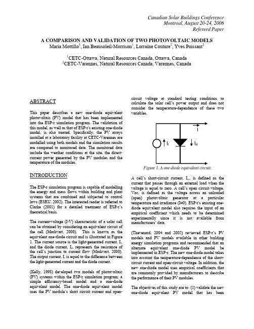
Canadian Solar Buildings ConferenceMontreal, August 20-24, 2006Refereed Paper A COMPARISON AND VALIDATION OF TWO PHOTOVOLTAIC MODELSMaria Mottillo1, Ian Beausoleil-Morrison1, Lorraine Couture2, Yves Poissant21CETC-Ottawa, Natural Resources Canada, Ottawa, Canada2CETC-Varennes, Natural Resources Canada, Varennes, CanadaABSTRACTThis paper describes a new one-diode equivalent photovoltaic (PV) model that has been implemented into the ESP-r simulation program. The validation of this model, as well as that of ESP-r's existing one-diode model, is also treated. Specifically, the PV arrays installed at a laboratory facility at CETC-Varennes are modelled using both models and the simulation results are compared to monitored data. The monitored data include the weather conditions at the site, the direct-current power generated by the PV modules and the temperature of the modules.INTRODUCTIONThe ESP-r simulation program is capable of modelling the energy and mass flows within building and plant systems that are combined and subjected to control laws (ESRU, 2002). The interested reader is referred to Clarke (2001) for a detailed treatment of ESP-r’s theoretical basis.The current-voltage (I-V) characteristic of a solar cell can be obtained by considering an equivalent circuit of the cell (Markvart, 2000). This is known as the equivalent one-diode circuit and is illustrated in Figure 1. The current source is the light-generated current, I l, and the diode current, I d, represents the resistance of the cell’s junction to current flow (Markvart, 2000). The output current, I, is equal to the difference between the light-generated current and the diode current. (Kelly, 1998) developed two models of photovoltaic (PV) systems within the ESP-r simulation program: a simple efficiency-based model and a one-diode equivalent model. The one-diode equivalent model uses the PV module’s short circuit current and open-circuit voltage at standard testing conditions to calculate the solar cell’s power output and does not consider the temperature-dependence of these two variables.Figure 1. A one-diode equivalent circuit.A cell’s short-circuit current, I sc, is defined as the current that passes through an external load when the voltage is equal to zero. A cell’s open circuit voltage, Voc, is defined as the voltage across an unloaded (open) photovoltaic generator at a particular temperature and irradiance (I=0). ESP-r's existing one-diode equivalent model also requires the input of an empirical coefficient which needs to be determined experimentally since it is not available from manufacturers’ data.(Thevenard, 2004 and 2005) reviewed ESP-r’s PV models and PV models available in other building energy simulation programs and recommended that an alternate equivalent one-diode PV model be implemented in ESP-r. The new one-diode model takes into account the temperature-dependence of the short-circuit current and open-circuit voltage. In addition, the new one-diode model uses empirical coefficients that are commonly provided by manufacturers to describe the performance of their PV modules.The objectives of this study are to: (1) validate the new one-diode equivalent PV model that has beenimplemented in ESP-r with monitored data; (2) validatethe existing PV model in ESP-r developed by (Kelly, 1998) with monitored data and (3) compare the simulation results obtained using both of ESP-r’s PV models.MATHEMATICAL MODELSThe new one-diode equivalent model implemented inESP-r is based on the WATSUN-PV model (Thevenard, 2004 and 2005). The WATSUN-PV model has an empirical basis and calculates the shortcircuit current, I sc , and open-circuit voltage, V oc , as follows:()[]ref c c ref effT ref sc sc T T E E I I ,,,1−+=α (1)()[]⎟⎟⎟⎠⎞⎜⎜⎜⎝⎛⎟⎟⎠⎞⎜⎜⎝⎛+⋅−−=ref eff T ref c c ref oc oc E E T T V V ,,,ln 10max 1βγ(2)where the subscript ref indicates reference conditions,E T,eff is the effective irradiance incident on the module(W/m 2), which includes the beam and diffuse components of solar radiation, taking into account thereflectance of the front surface of the module. Tc is thecell temperature (°C) and α, γ and β are empiricalcoefficients. The empirical coefficients in equations (1)and (2) are provided in the specifications for many PVmodules, as are I sc,ref and V oc,ref . Standard referenceconditions are E ref = 1000 W/m 2 and T c,ref = 25°C.The WATSUN-PV model assumes that the maximumpower point voltage, V mp , and the maximum powerpoint current, I mp , vary proportionately with the short-circuit current and open circuit voltage and thereforethe maximum power, P mp is given by equation (3):⎟⎟⎠⎞⎜⎜⎝⎛⋅⋅⋅=ref oc ref sc oc sc ref mp ref mp mp V I V I V I P ,,,, (3)This assumption is a weakness of the WATSUN-PVmodel since in practice, the shape factor mp mp ocsc V I V Iis not constant; it varies with temperature andirradiance (Thevenard, 2004). The parameters I mp,refand V mp,ref of equation (3) are available frommanufacturers’ specifications.In this study, the PV modules operate at maximum power point and therefore equations (1) – (3) are the only equations used by the WATSUN-PV model to calculate the power output of the modules.ESP-r's existing one-diode equivalent model does not consider the temperature-dependence of the short-circuit current and open-circuit voltage; rather, theshort-circuit current and open-circuit voltage atreference conditions are used to calculate the power output of the PV module. In addition, this model requires an empirical constant whose value varies with the characteristics of the PV material. This empiricalconstant is not available from manufacturers’ data, but rather is to be found by laboratory testing. In ESP-r, the PV module surface is represented as a multi-layered construction consisting of several material layers. Each layer is represented with one or more nodes. One node within the surface is identified as a special material node; this node represents the location of the PV cells within the module. The cell temperature Tc is determined by considering the energy balance of the special material node. It should be noted that the solar radiation absorbed by the special material node is reduced by the power generated fromthe node. MONITORED DATA The monitored data for two PV arrays installed at a laboratory facility at CETC-Varennes are used in this study. The PV modules installed at CETC-Varennes are multicrystalline silicon modules from AstroPower (model APC 5103). The characteristics of the modules are provided in Table 1; reference conditions are 1000 W/m 2, 25°C and air mass 1.5. Each of the two arrays is made up of several modules connected in series and parallel and rack mounted on the building roof at an angle of 45°. Both arrays face due south. The characteristics of each array (identified as A and B) are provided in Table 2. The following data are collected at CETC-Varennes: • voltage (V) of high tension sections of arrays (each array is separated into a high tension section and a low tension section); • voltage (V) of low tension sections of arrays; • current (A) of high tension sections of arrays;• low current (A) of arrays A;•DC power (W) generated by arrays (input to DC-AC inverter);•AC power (W) delivered by arrays (output from DC-AC inverter);•temperature (°C) of arrays (sensors are placed at the center of each high- and low- tension section of each array);•global irradiance on the horizontal (W/m 2); •direct normal irradiance (W/m 2);•diffuse irradiance on the horizontal (W/m 2); •total irradiance (W/m 2) at 45°; •ambient temperature (°C); •relative humidity (%); •wind speed (km/h) and•wind direction (degrees clockwise from north).Table 1. Description of PV modulesModule length (mm) 959.5Module width (mm) 395.0Number of cells in series 36Number of cells in parallel 1V oc,ref (V) 20.37I sc,ref (A) 3.02V mp,ref (V) 15.32I mp,ref (A) 2.7Table 2. PV array characteristicsArray A Array BNumber of modules 140 112Area (m 2) 56.0 44.8The data are recorded every 15 seconds. For thisanalysis, the recorded data are averaged over 15-minute intervals for four representative days: June 27(2005) represents a hot, sunny summer day; January 21(2005) represents a cold, sunny winter day; July 9 (2005) represents a cloudy summer day and July 2(2005) represents a sunny summer day. These fourdays were chose since they represent different temperature and sunny/cloudy conditions.SIMULATION INPUTSHourly weather files for the four representative dayswere created from the monitored data in the formatrequired by ESP-r. The solar radiation data specified inthe weather files are the direct normal irradiance and diffuse horizontal irradiance per hour.The characteristics provided in Tables 1 and 2, obtained from CETC-Varennes, are used to describe the PV arrays in ESP-r, for both the WATSUN-PV model and Kelly’s PV model. The empirical coefficients required by the WATSUN-PV model, provided in Table 3, have been determined by (Thevenard, 1999) experimentally. Specificially, (Thevenard, 1999) measured I-V curves for various temperature and insolation conditions and used non-linear curve-fitting algorithms to determine the module parameters (short-circuit current, open-circuit voltage, maximum power point current and voltage) and empirical coefficients. Although for this analysis, the module parameters and empirical coefficients required by the WATSUN-PV model were obtained from experimental data, since the latter were available, the module parameters and empirical coefficients required by the model are available from manufacturers’ specifications. Table 3. Empirical coefficients required by WATSUN-PV model for modules A and B (Thevenard, 1999). Array A Array B α (/°C) -8.310E-05 -8.267E-06 γ(/°C) 0.00355 0.00344 β 0.0054 0.0681 Since the laboratory test data were not available to determine the empirical constant required by Kelly’s PV model, the default value (σ = 10) is used for the simulations. The empirical constant required by Kelly’s PV model affects the power output of the PV module through its influence on the calculation of the diode current (Kelly, 1998). The default value used in this study is used by (Buresch, 1983). The implementation of the WATSUN-PV model in ESP-r allows the miscellaneous power losses from thePV modules due to uncertainty in the module ratings, ageing, soil and dirt, mismatch, snow, blocking diodes and wiring to be considered. However, these factorsare ignored in the simulations reported here since theyare difficult to quantify. The construction of the arrays is assumed to be typical of PV installations. The overall U-value of the PV module used in the simulations is 5.27 W/ m 2°C. Aground reflectance (albedo) of 0.2, the default value, is used in the simulations.Each PV array is modelled in ESP-r as a thin zone; the zone is made up of one surface which represents the PV modules, with the remaining surfaces defined as an aluminium layer representing the array’s aluminium frame. The interior convection coefficient for the PV module surface is set to a high value (10 W/m 2°C), as is the zone’s infiltration rate, and no casual gains are defined in the zones. Simulations are carried out for the four representative days using 15-minute time-steps.SIMULATION RESULTSFigures 2 to 5 compare the DC power produced by array A, as predicted by the WATSUN-PV and (Kelly, 1998) models, to the actual power produced for the four representative days considered in this study.Figure 2. DC Power generation of Array A on June 27Figure 3. DC Power generation of Array A on January 21Figure 4. DC Power generation of Array A on July 9Figure 5. DC Power generation of Array A on July 2Figures 2-5 suggest that both of ESP-r’s PV models correctly predict the shape of the power generation-versus-time curve. However, both models tend to over-predict the power generated by the PV arrays at mid-day, particularly on the sunny days (June 27, January 21 and July 2). The results of the WATSUN-PV model and Kelly model are similar but the latter model seems to over-predict the power generation to a lesser degree on the sunny days. The power predictions for Array B, not presented, are similar to those of Array A.Figures 6-9 provide the predicted surface temperatures of PV array A, the measured average temperatures of array A (average of measurements taken at two different locations on the array) and the outdoor temperatures for the four representative days considered in this study. It should be noted that both of ESP-r’s PV models use the same algorithm todetermine the temperatures of the array surfaces.Canadian Solar Buildings Conference Montreal, August 20-24, 2004Refereed PaperFigure 7. Temperatures of Array A on January 21 Figure 6. Temperatures of Array A on June 27Figure 7. Temperatures of ArrayA on January 21Figure 8. Temperatures of Array A on July 9Figure 9. Temperatures of Array A on July 2 On the sunny summer days (June 27 and July 2), the surface temperatures of the array predicted by ESP-r during the night are close to the outdoor temperatures, as one would expect. On the cold, sunny day (January 21), the surface temperatures predicted by ESP-r are close to the average monitored temperatures except at mid-day. On the cloudy, summer day (July 9), the predicted surface temperatures are approximately 5°C higher than the average monitored temperatures. However, the predicted surface temperatures are close to the one of the monitored temperature readings (shown as ‘Temp 1’ in Figure 8), suggesting that there may be some errors in the temperature measurements and the average of the two monitored temperatures may not be representative of the array temperature. It is not expected that the small differences between the predicted surface temperatures and the monitored temperatures will significantly impact the predictions of the power generated by the array.ANALYSISIn order to identify the possible sources of the discrepancies between the predicted and actual DC power generation of the PV arrays, simulations of the arrays were carried out in TRNSYS (SEL, 2004). The solar radiation data input to TRNSYS includes the global horizontal irradiance and diffuse horizontal irradiance per hour. In order to correctly compare the TRNSYS and ESP-r simulation results, the same solar radiation is input to ESP-r, that is the global horizontal irradiance and diffuse horizontal irradiance per hour (previous ESP-r simulation results were obtained using the direct normal irradiance and diffuse horizontal irradiance per hour). The PV model in TRNSYS is based on a one-diode equivalent electrical circuit and the concept of nominal operating cell temperature (NOCT).Figures 10-13 compare the predicted DC power generation of array A by (1) the WATSUN-PV model when the solar radiation data are defined using the direct normal irradiance and diffuse horizontal irradiance (WATSUN-PV:DR label), (2) the WATSUN-PV model when the solar radiation data are defined using the global horizontal irradiance and diffuse horizontal irradiance (WATSUN-PV:Glob label), (3) the TRNSYS PV model and (4) the actual DC power generation measured by the data acquisition system. The DC power generation predicted for array Bis similar to that of array A and therefore not presented in this study.Figure 10. DC Power generation of Array A on June 27Figure 11. DC Power generation of Array A on January 21Figure 12. DC Power generation of Array A on July 9Figure 13. DC Power generation of Array A on July 2 On the two warm sunny days (June 27 and July 2), the WATSUN-PV model more accurately predicts the DC power generated by array A when the global horizontal irradiance and diffuse horizontal irradiance are specified in the weather file. On these days, the WATSUN-PV simulation results agree with the TRNSYS simulation results and the monitored data. On the cold winter day (January 21) and the cloudy summer day (July 9), the DC power generation predicted by TRNSYS does not agree with the monitored data and no difference is seen in the WATSUN-PV results whether the direct normal irradiance or global horizontal irradiance is used to specify the solar radiation data in ESP-r.Since there is no pattern to the disagreement between the measured values and the different simulation results, a comparison of the measured versus predicted total irradiance on the tilted array is carried out next. Figures 14-17 present the total irradiance on the tilted array A for the four representative days as predicted by ESP-r (using either the direct normal irradiance or global horizontal irradiance in the weather file) and TRNSYS and measured by the pyranometer at CETC-Varennes.Figure 14. Total irradiance on Array A on June 27Figure 15. Total irradiance on Array A on January 21Figure 16. Total irradiance on Array A on July 9Figure 17. Total irradiance on Array A on July 2On the sunny summer days (June 27 and July 2), the irradiance on the tilted array predicted by TRNSYS is lower than the measured irradiance. This is also the case in ESP-r when the global horizontal irradiance, versus the direct normal irradiance, is specified in the weather file. In ESP-r, the predicted irradiance agrees with the monitored data when the direct normal irradiance is specified. This pattern is not reflected in the results for the cold sunny winter day (January 21) or for the cloudy summer day (July 9). The question arises whether there are errors with the monitored data since the irradiance on the tilted surface that is calculated by ESP-r should be the same whether the direct normal or the global horizontal irradiance is specified in the weather file; this is the case for the cold winter day and for the cloudy summer day but not for the sunny summer days.The results of this study are inconclusive and further work is required to validate the PV models within ESP-r. Specifically, a verification of the monitored data used in this study is required and/or another set of monitored data should be used in future validation work. In addition, a verification of ESP-r’s source code with respect to the calculation of the irradiance on a tilted surface should be carried out and compared to TRNSYS’s algorithm.CONCLUSIONThis study is a first attempt to validate the new one-diode equivalent model, based on the WATSUN-PV model, that has been implemented in ESP-r and the existing one-diode equivalent model, developed by (Kelly, 1998).The simulation results using (Kelly, 1998)’s PV model are comparable to the simulation results obtained using the WATSUN-PV model, when comparing the simulation results with monitored data. Both of ESP-r’s one-diode equivalent PV models correctly predict the shape of the power-versus-time curve for the four representative days considered in this study. However, the ESP-r models over-predict the amount of DC power generated at mid-day, especially on the sunny days.The temperatures of the arrays predicted by the models are within an acceptable range of difference with the monitored data. It is not expected that resolving the differences between the predicted and actual temperatures will impact the predicted power generation significantly.The PV arrays were modelled with the TRNSYS software in order to identify any possible sources of error with ESP-r’s PV models. The results of the TRNSYS simulations for the sunny summer days agree well with the monitored data and with the results of the WATSUN-PV model when the global horizontal irradiance, versus the direct normal irradiance, is used to specify the solar radiation data in ESP-r. On the cold winter day and cloudy summer day, neither ESP-rnor TRNSYS predicted the power generation of the PV arrays very well.The total irradiance on the tilted array predicted by ESP-r and TRNSYS is less than the monitored data on the sunny summer days when the global horizontal, versus the direct normal, irradiance is used to specify the solar radiation data.The comparisons between the predicted and actual DC power generation of the PV arrays are inconsistent for the four representative days considered in this study. Since the comparisons of the predicted and actual array temperatures and surface irradiances are also inconsistent, the validity of ESP-r’s PV models is inconclusive. It is recommended that further validation of ESP-r’s PV models be carried out in the future. In particular, it is recommended that (1) the monitored data used in this study be verified, specifically that a quality check on the global horizontal, diffuse horizontal and direct normal measurements be performed and (2) that another set of monitored data be used for future work . Future work should also focus on using a full year, in addition to representative days, of monitored data to validate ESP-r’s PV models. REFERENCESBuresch M. (1983), Photovoltaic energy systems – design and installation, McGraw-Hill, New York.Clarke J.A. (2001), Energy Simulation in Building Design, 2nd Edition, Butterworth-Heinemann, Oxford, UK.Energy Systems Research Unit (ESRU) (2002), The ESP-r System for Building Energy Simulations: User Guide Version 10), ESRU Manual U02/1, University of Strathclyde, Glasgow, U.K.Kelly, N. (1998), Towards a Design Environment for Building Integrated Energy Systems: The Integration of Electrical Power Flow Modelling with Building Simulation, Ph.D. dissertation, University of Strathclyde, Glasgow, U.K. Markvart, T. (2000), Solar Electricity, 2nd Edition, John Wiley & Sons, New York.Solar Energy Laboratory (SEL) (2004), TRNSYS Version 16, University of Wisconsin, Madison, U.S.A. Thevenard, D. (1999), ‘Energy Rating of PV Modules (August 1999 Report)’, Internal Report, CETC-Varennes, Natural Resources Canada.Thevenard, D. (2004), ‘Literature Review and Source Code Review of ESP-r’s Existing Photovoltaic (PV) Models’, Internal Report, CETC-Ottawa, Natural Resources Canada.Thevenard, D. (2005), ‘Review and Recommendationsfor Improving the Modelling of Building Integrated Photovoltaic Systems’, Proceedings of Building Simulation 2005, Montréal, Canada, 1221-1228. NOMENCLATUREI Current {Amps} V Voltage {Volts} T Temperature {°C}E Irradiance {W/m2}P Power {Watts} αTemperature coefficient of I sc {°C-1}βTemperature coefficient of V oc {°C-1}γIrradiance coefficient of V ocσEmpirical coefficient used by (Kelly, 1998) Subscriptsref Referencel Light-generatedd Diodesc Short-circuitoc Open-circuiteff Effectivec Cellmp Maximumpower-point。
搅拌摩擦焊的工艺参数

Trans. Nonferrous Met. Soc. China 22(2012) 1064í1072Correlation between welding and hardening parameters offriction stir welded joints of 2017 aluminum alloyHassen BOUZAIENE, Mohamed-Ali REZGUI, Mahfoudh AYADI, Ali ZGHALResearch Unit in Solid Mechanics, Structures and Technological Development (99-UR11-46),Higher School of Sciences and Techniques of Tunis, TunisiaReceived 7 September 2011; accepted 1 January 2011Abstract: An experimental study was undertaken to express the hardening Swift law according to friction stir welding (FSW) aluminum alloy 2017. Tensile tests of welded joints were run in accordance with face centered composite design. Two types of identified models based on least square method and response surface method were used to assess the contribution of FSW independent factors on the hardening parameters. These models were introduced into finite-element code “Abaqus” to simulate tensile tests of welded joints. The relative average deviation criterion, between the experimental data and the numerical simulations of tension-elongation of tensile tests, shows good agreement between the experimental results and the predicted hardening models. These results can be used to perform multi-criteria optimization for carrying out specific welds or conducting numerical simulation of plastic deformation of forming process of FSW parts such as hydroforming, bending and forging.Key words: friction stir welding; response surface methodology; face centered central composite design; hardening; simulation; relative average deviation criterion1 IntroductionFriction stir welding (FSW) is initially invented and patented at the Welding Institute, Cambridge, United Kingdom (TWI) in 1991 [1] to improve welded joint quality of aluminum alloys. FSW is a solid state joining process which was therefore developed systematically for material difficult to weld and then extended to dissimilar material welding [2], and underwater welding [3]. It is a continuous and autogenously process. It makes use of a rotating tool pin moving along the joint interface and a tool shoulder applying a severe plastic deformation [4].The process is completely mechanical, therefore welding operation and weld energy are accurately controlled. B asing on the same welding parameters, welding joint quality is similar from a weld to another.Approximate models show that FSW could be successfully modeled as a forging and extrusion process [5]. The plastic deformation field in FSW is compared with that in metal cutting [6í8]. The predominant deformation during FSW, particularly in vicinities of thetool, is expected to be simple shear, and parallel to the tool surface [9]. When the workpiece material sticks to the tool, heat is generated at the tool/workpiece contact due to shear deformation. The material becomes in paste state favoring the stirring process within the thermomechanically affected zone, causing a large plastic deformation which alters micro and macro structure and changes properties in polycrystalline materials [10].The development of the mechanical behavior model, of heterogeneous structure of the welded zone, is based on a composite material approach, therefore it must takes into account material properties associated with the different welded regions [11]. The global mechanical behavior of FSW joint was studied through the measurement of stress strain performed in transverse [12,13] and longitudinal [14] directions compared with the weld direction. Finite element models were also developed to study the flow patterns and the residual stresses in FSW [15]. B ased on all these models, numerical simulations were performed in order to investigate the effects of welding parameters and tool geometry on welded material behaviors [16] to predict the feasibility of the process on various shape parts [17].Corresponding author: Mohamed-Ali REZGUI; E-mail: mohamedali.rezgui@ DOI: 10.1016/S1003-6326(11)61284-3Hassen BOUZAIENE, et al/Trans. Nonferrous Met. Soc. China 22(2012) 1064í1072 1065 However, the majority of optimization studies of theFSW process were carried out without being connectedto FSW parameters.In the present study, from experimental andmodeling standpoint, the mechanical behavior of FSWaluminum alloy 2017 was examined by performingtensile tests in longitudinal direction compared with theweld direction. It is a matter of identifying the materialparameters of Swift hardening law [18] according to theFSW parameters, so mechanical properties could bepredicted and optimized under FSW operating conditions.The strategy carried out rests on the response surfacemethod (RSM) involving a face centered centralcomposite design to fit an empirical models of materialparameters of Swift hardening law. RSM is a collectionof mathematical and statistical technique, useful formodeling and analysis problems in which response ofinterest is influenced by several variables; its objective isto optimize this response [19]. The diagnostic checkingtests provided by the analysis of variance (ANOV A) suchas sequential F-test, Lack-of-Fit (LoF) test, coefficient ofdetermination (R2), adjusted coefficient of determination(2adjR) are used to select the adequacy models [20].2 Experimental2.1 Welding processThe aluminum alloy 2017 chosen for investigationhas good mechanical characteristics (Table 1), excellentmachinability and formability, and is mostly used ingeneral mechanics applications from high strengthsuitable for heavy-duty structural parts.Table 1 Mechanical properties of aluminum alloy 2017Ultimate tensile strength/MPaYieldstrength/MPaElongation/%Vickershardness427 276 22 118 The experimental set up used in this study was designed in Kef Institute of Technology (Tunisia). A 7.5 kW powered universal mill (Momac model) with 5 to 1700 r/min and welding feed rate ranging from 16 to 1080 mm/min was used. Aluminum alloy 2017 plate of6 mm in thickness was cut and machined into rectangular welding samples of 250 mm×90 mm. Welding test was performed using two samples in butt-configuration, in contact along their larger edge, fixed on a metal frame which was clamped on the machine milling table.To ensure the repeatability of the FSW process, clamping torque and flatness surface of the plates to be welded are controlled for each welding test. At the end of welding operation, around 80 s are respected before the withdrawal of the tool and the extracting of the welded parts. In this experimental study, we purpose to screen theeffects of three operating factors, i.e. tool rotational speed N, tool welding feed F and diameter ratio r, on hardening parameters from Swift’s hardening law such as strength coefficient (k), initial yield strain (İ0) and hardening exponent (n). The ratio (r=d/D) of pin diameter (d) to shoulder diameter (D), is intended to optimize the tool geometry [21í23]. The welding tool is manufactured from a high alloy steel (Fig. 1).Fig. 1 FSW tool geometry (mm)Preliminary welding tests were performed to identify both higher and lower levels of each considered factors. These limits are fixed from visual inspections of the external morphology and cross sections of the welded joints with no macroscopic defects such as surface irregularities, excessive flash, and lack of penetration or surface-open tunnels. However, among these limits one is not sure to have a safe welded joint so often, but they show great potential on defect avoidance. Figure 2 shows some external macroscopic defects observed beyond the limit levels established for each factor. Table 2 lists the processing factors as well as levels assigned to each, and Table 3 shows the fixed levels for other factors needed to success the welding tests.A face centered central composite design, which comes under the RSM approach, with three factors was used to characterize the nature of the welded joints by determining hardening parameters. In this design the star points are at the center of each face of the factorial space (Į=±1), all factors are run at three levels, which are í1, 0, +1 in term of the coded values (Table 4). The experiment plan has been run in random way to avoid systematic errors.2.2 Tensile testsThe tensile tests are performed on a Testometric’s universal testing machines FSí300 kN. The tensile test specimens (ASME E8Mí04) proposed for characterizing the mechanical behavior of the FSW joint, were cut inHassen BOUZAIENE, et al/Trans. Nonferrous Met. Soc. China 22(2012) 1064í10721066Fig. 2 Types of macroscopic defectsTable 2 Levels for operating parameters for FSW processFactorLow level (í1) Center point (0) High level(+1)N /(r·min í1) 653 910 1280 F /(mm·min í1)67 86 109r /%33 39 44Table 3 Welding parametersPin height/ mm Shoulder diameter/ mm Small diameter pin/mm Tool’s inclination angle/(°) Penetrationdepth of shoulder/mm5.3 18 4 30.78longitudinal direction compared with the weld direction, so that active zone is enclosed in the central weld zone (Fig. 3). Figure 4 shows the tensile specimens after fracture.Ultimately, it is a matter of experimental evaluation of hardening parameters of the behavior of FSW joints (k , İ0, n ) according to Swift’s hardening law:n k )(p 0H H V (1)These parameters are required to identify the plastic deformation aptitude of the FSW joints. They are also needed for numerical simulations of forming operations on welded plates. The hardening parameters have been calculated by least square method (LSM) from the stressüstrain curves data. Table 4 shows the experimental design as well as dataset performance characteristics according to the FSW parameters of aluminum Alloy 2017.3 Experimental results3.1 Development of mathematical modelsAlthough the basic principles of FSW are very simple, it involves complex phenomena related to thermo-mechanical and metallurgical transformation that causes strong microstructural heterogeneities in the welded zone. From an energy standpoint, welding process is generated by converting mechanical energy provided by FSW tool into other types of energy such as heat, plastic deformation and microstructural transformations. The nonlinear character of these different dissipation forms can justify research for nonlinear prediction models whose accuracy generally depends on the order of the models relating the responses to welding parameters. For this reason, we chose the RSM which is helpful in developing a suitable approximation for the true functional relationships between quantitative factors (x 1, x 2, Ă, x k ) and the response surface or response functions Y (k , İ0, n ) that may characterize the nature of the welded joints as follows:r 21),,,(e x x x f Y k (2)Hassen BOUZAIENE, et al/Trans. Nonferrous Met. Soc. China 22(2012) 1064í10721067Table 4 Face centered central composite design for FSW of aluminum alloy 2017Factors levelCoded Actual Hardening parameterTypeStandard orderN F r N /(r·m í1)F /(mm·min í1)r /% k /MPan İ0/%1 í1 í1 í165367 33629.7 0.3296 0.00202 1 í1 í1 1280 67 33 654.7 0.4514 0.0035 3 í1 1 í1 653109 33 587.8 0.3712 0.0025 4 1 1 í1 1280 109 33 689.2 0.4856 0.00555 í1 í1 1 653 67 44 642.3 0.4524 0.00256 1 í1 1128067 44 218.6 0.2447 0.0015 7 í1 1 1 653 109 44 685.5 0.4885 0.0035 Factorialdesign8 1 1 1 1280 109 44 332.5 0.3405 0.00209 0 0 0 91086 39 624.9 0.4257 0.0025 10 0 0 0 910 86 39 639.9 0.4292 0.0025 11 0 0 0 910 86 39 640.9 0.4011 0.0020 Center point12 0 0 0 910 86 39 598.6 0.3960 0.0023 13 í1 0 0 653 86 39 690.6 0.4748 0.0027 14 1 0 0 128086 39 505.6 0.3909 0.0030 15 0 í1 091067 39499 0.3317 0.001716 0 1 0 910 109 39 545.6 0.4157 0.0026 17 0 0 í1 910 86 33 672.1 0.4385 0.0027 Star point18 0 019108644 509.7 0.41750.0019Fig. 3 Tensile test specimens (ASME E8Mí04) cut in longitudinal direction compared with weld direction (mm)Fig. 4 Tensile specimens after fractureThe residual error term (e r ) measures theexperimental errors. Such relationship was developed as quadratic polynomial under multiple regression form [19,20]:¦¦¦ r 20e x x b x b x b b Y j i ij i ii i i (3)where b 0 is an intercept or the average of response; b i , b ii , and b ij represent regression coefficients. For the three factors, the selected polynomial could be expressed as:2332222113210r b F b N b r b F b N b b YFr b Nr b NF b 231312 (4)In applying the RSM, the independent variable Y was viewed as surface to which a mathematical model was fitted. The adequacy of the developed model was tested using the analysis of variance (ANOV A) which quantifies the amount of variation in a process and determines if it is significant or is caused by random noise.3.2 Mathematic model of hardening parametersTable 5 lists the coefficients of the best linear regression models. All selected parameters (N , F , r ) for k and İ0 are statistically significant (P-value less than 0.05) at the 95% confidence level. However, for the response n , the term b 3r having a P-value=0.0654>0.05 is not statistically significant at the 95% confidence level even though the term b 13Nr is statistically significant. Consequently, b 3(r ) is kept in the model to improve the Lack-of-Fit test (Table 6). Furthermore, only theHassen BOUZAIENE, et al/Trans. Nonferrous Met. Soc. China 22(2012) 1064í10721068Table 5 Coefficients of regression models for hardening parametersStrength coefficient (k) Hardeningcoefficient(n) Initial yield strain (İ0) CoefficientEst. SEP-value Est SE P-valueEst/10í4 SE/10í4 P-value b0 610.39,48<10í4 0.422 0.0073 <10-4 22.8 1.010 <10-4 b1 í83.58.48<10í4 í0.020 0.0065 0.0091 2.30 0.912 0.0267 b2 19.68.480.0410.0290.00650.00084.900.9120.0002b3 í84.58.48<10í4 í0.013 0.0065 0.0654 í4.80 0.912 0.0002 b11 5.561.3670.0009b22 í61.812.720.0005í0.0310.00980.009b33b12b13 í112.99.48<10í4 í0.074 0.0073 <10-4 -8,75 1.010 <10-4 b23R2 95.90% 92.38% 92.84%2adjR 94.19% 89.21% 89.86% SE of est. 30.7 0.021 2.9×10í4Est: Estimate; SE: Standard Error; SE of est.: Standard error of estimateTable 6 ANOV A for hardening parametersk n İ0Source of variationSS Df P-Value SS Df P-Value SS/10í7 Df P-Value Model 263946.0 5 <10í4 0.062357 5 <10í4 129.324 5 <10í4Residual 11296.4 12 0.005140912 9.97 12Lack-of-Fit 10130.4 9 0.2065 0.00428669 0.3678 8.295 9 0.3723 Pure error 1166.07 3 0.0008543 3 1.675 3 Total correction 275243.017 0.06749817 139.294 17 DW-value 1.31 1.42 2.26DW: Durbin-Watson statistic; SS: Sum of squares; D f: Degree of freedominteraction (Nír) is statistically significant on the three responses (Fig. 5). According to the adjusted R2 statistic, the selected models explain 94.19%, 89.21% and 89.86% of the variability in k, n and İ0 respectively.The ANOV A (Table 6) for the hardening parameter shows that all models (k, n, İ0) represent statistically significant relationships between the variables in each model at the 99% confidence level (P-value<10í4). The Lack-of-Fit test confirms that these models (k, n, İ0) are adequate to describe the observed data (P-value>0.05) at the 95% confidence level. The DW statistic test indicates that there is probably not any serious autocorrelation in their residuals (DW-value>1.4). The normal probability plots of the residuals suggest that the error terms, for these models, are indeed normally distributed (Fig. 6). The response surface models in terms of coded variables (Eqs. (5)í(7)) are shown in Fig. 7.k=610.3–83.5 N+19.6 F–84.5 r –61.8 F2–112.9 Nr(5) n=0.422–0.020 N+0.029 F–0.013 r–0.031 F2–0.074 Nr(6) İ0=22.8+2.3 N+4.90 F–4.80 r+5.56 N2–8.75 Nr(7) Fig. 5 Interaction plots of Nír (rotational speedídiameter ratio): (a) Strength coefficient k; (b) Hardening coefficient n;(c) Initial yield strain İ0Hassen BOUZAIENE, et al/Trans. Nonferrous Met. Soc. China 22(2012) 1064í1072 1069Fig. 6 Normal probability plots for residual: (a) Strength coefficient k; (b) Hardening coefficient n; (c) Initial yield strain İ04 Validation of identified modelsValidation tests of the identified models were performed through comparative study between the experimental models (EM) of tensile tests and the computed responses given by numerical simulations of the same tests (Fig. 8). The computed responses, expressed in the form of tension and elongation, wereFig. 7 Response surfaces plots: (a) Strength coefficient k;(b) Hardening coefficient n; (c) Initial yield strain İ0 established by examining welded joints having an elastoplastic behavior in accordance with the Swift hardening law (Eq. (1)). These computed responses were deduced from the numerical simulations using the finite element code Abaqus/Implicit, in which the introduced elastoplastic behavior was obtained from the least square hardening models (LSHM) (Table 4) and the response surface hardening models (RSHM) (Table 5). The highest deviations (<10%), between EM and computed response, were recorded with the RSHM. Increasing deviations, as shown in Fig. 8, is due to the effect of combining damage with plastic strains accumulatedHassen BOUZAIENE, et al/Trans. Nonferrous Met. Soc. China 22(2012) 1064í10721070Fig. 8 Relationship between tension and elongation: Confrontation between experimental model (EM), and computed responses (LSHM, RSHM) for three experimental testsduring the onset of localized necking.The relative average deviation criterion (EM/LSHM ]) between the experimental data and the numerical predictions of tensions, was used to assess the quality of the identified models.¦¸¸¹·¨¨©§'' '2exp num exp exp/num )()()(1i i i L F L F L F N] (8)where N is the number of experimental measurements,F exp (ǻL i ) and F num (ǻL i ) are respectively the experimental and predicated tensions relating to the i-th elongation ǻL i . Figure 9 illustrates that the relative average deviation of EM/LSHM (EM/LSHM ]) ranges between 1.64% and 6.75% while the relative average deviation of EM/RSHM (EM/RSHM ]) ranges between 4.52% and 9.32%.Fig. 9 Distribution of relative average deviations for most representative experimental testsFor the deviation within limits fluctuating between 4.52% and 6.75% the estimated models (LSHM and RSHM) are comparable. This applies particularly to welded joints characterized by a strength coefficient (k ), ranging from 520 to 610 MPa and a hardening exponent (n ) ranging between 0.30 and 0.45.5 DiscussionIn this study we evaluated, using RSM, the effect of FSW parameters such as tool rotational speed, welding feed rate and diameter ratio of pin to shoulder on the plastic deformation aptitudes of welded joints. The performed analysis highlights the incontestable significant effects of rotational speed (N ), welding feed rate (F ) and the interaction (Nír ) between rotational speed and diameters ratio on hardening parameters (k , n , İ0) according to Swift law. The established models show that tool diameter ratio has a linear effect only on (k ) and (İ0), it does not have any quadratic effect. They also show that rotational speed has a quadratic effect solely on (İ0); while welding feed rate has a quadratic effect on both (k ) and (n ).In addition, numerical simulation of tensile tests of welded joints has been made possible through the predictive models (LSHM and RSHM) of Swift’s hardening parameters. To judge whether the models represent correctly the data, a comparative study between the experimental response and the computed response, expressed in terms of tension-elongation, was carried out. It was found that the relative average deviation betweenHassen BOUZAIENE, et al/Trans. Nonferrous Met. Soc. China 22(2012) 1064í1072 1071experimental model and numerical models is less than 9.5% in all cases.Moreover, correlation between welding and hardening parameters provided has many benefits. The correlation relationships can solve inverse problem relating to optimal choice of parameters linked up with the desired welded joints properties to produce welds having tailor-made mechanical properties. The correlation predictions offer the possibility to identify the behavior of friction stir welded joints necessary for finite element simulations of various forming processes while minimizing experimental cost and time. Ultimately, understanding correlations can be useful for studies on reliability of welded assemblies in service life expectancy.6 Conclusions1) Rotational speed and welding feed rate are the factors that have greater influence on hardening parameters (k, n, İ0), followed by diameter ratio that has no influence on the hardening coefficient (n).2) The numerical models RSHM were compared with those through LSHM and confronted to the experimental results. Indeed, within the limit of a relative average deviation of about 9.3%, between the experimental model and numerical models expressed in terms of tension-elongation, the validity of these models is acceptable.3) The predictive models of work-hardening coefficients, established taking into account the FSW parameters, have made possible the numerical simulation of tensile tests of FSW joints. These results can be used to perform multi-criteria optimization for producing welds with specific mechanical properties or conducting numerical simulation of plastic deformation of forming process of friction stir welded parts such as hydroforming, bending and forging.References[1]THOMAS W M, NICHOLAS E D, NEEDHAM J C, MURCH M G,TEMPLE-SMITH P, DAWES C J. Friction stir butt welding,PCT/GB92/ 02203 [P]. 1991.[2]XUE P, NI D R, WANG D, XIAO B L, MA Z Y. Effect of friction stirwelding parameters on the microstructure and mechanical propertiesof the dissimilar AlíCu joints[J]. Materials Science and EngineeringA, 2011, 528: 4683í4689.[3]LIU H J, ZHANG H J, YU L. Effect of welding speed onmicrostructures and mechanical properties of underwater friction stirwelded 2219 aluminum alloy [J]. Materials and Design, 2011, 32:1548í1553.[4]MISHRA R S, MA Z Y. Friction stir welding and processing [J].Materials Science and Engineering R, 2005, 50: 1í78.[5]ARB EGAST W J. A flow-partitioned deformation zone model fordefect formation during friction stir welding [J]. Scripta Materialia,2008, 58: 372í376.[6]LEWIS N P. Metal cutting theory and friction stir welding tooldesign [M]. NASA Faculty Fellowship Program Marshall SpaceFlight Center, University of ALABAMA, NASA/MSFC Directorate:Engineering (ED-33), 2002.[7]ARB EGAST W J. Modeling friction stir welding joining as ametalworking process, hot deformation of aluminum alloys III [C].San Diego: TMS Annual Meeting, 2003: 313í327.[8]ARTHUR C N Jr. Metal flow in friction stir welding [R]. NASAmarshall space flight center, EM30. Huntsville, AL 35812.[9]FONDA R W, B INGERT J F, COLLIGAN K J. Development ofgrain structure during friction stir welding [J]. Scripta Materialia,2004, 51: 243í248.[10]NANDAN R, DEBROY T, BHADESHIA H K D H. Recent advancesin friction stir weldingüProcess, weldment structure and properties[J]. Progress in Materials Science, 2008, 53: 980í1023.[11]LOCKWOOD W D, TOMAZ B, REYNOLDS A P. Mechanicalresponse of friction stir welded AA2024: Experiment and modeling[J]. Materials Science and Engineering A, 2002, 323: 348í353. [12]SALEM H G, REYNOLDS A P, LYONS J S. Microstructure andretention of superplasticity of friction stir welded superplastic 2095sheet [J]. Scripta Materialia, 2002, 46: 337í342.[13]LOCKWOOD W D, REYNOLDS A P. Simulation of the globalresponse of a friction stir weld using local constitutive behavior [J].Materials Science and Engineering A, 2003, 339: 35í42.[14]SUTTON M A, YANG B, REYNOLDS A P, YAN J. B andedmicrostructure in 2024–T351 and 2524-T351 aluminum friction stirwelds, Part II. Mechanical characterization [J]. Materials Science andEngineering A, 2004, 364: 66í74.[15]ZHANG H W, ZHANG Z, CHEN J T. The finite element simulationof the friction stir welding process [J]. Materials Science andEngineering A, 2005, 403: 340í348.[16]ZHANG Z, ZHANG H W. Numerical studies on controlling ofprocess parameters in friction stir welding [J]. Journal of MaterialsProcessing Technology, 2009, 209: 241í270.[17]B UFFA G, FRATINI L, SHIVPURI R. Finite element studies onfriction stir welding processes of tailored blanks [J]. Computers andStructures, 2008, 86: 181í189.[18]SWIFT H W. Plastic instability under plane stress [J]. Journal of theMechanics and Physics of Solids, 1952, 1: 1í18.[19]MONTGOMERY D C. Design and analysis of experiments [M].Fifth Edition. New York: John Wiley & Sons, 2001: 684.[20]MYERS R H, MONTGOMERY D C, ANDERSON-COOK C M.Response surface methodology: Process and product optimizationusing designed experiment [M]. 3rd Edition. New York: John Wiley& Sons, 2009: 680.[21]VIJAY S J, MURUGAN N. Influence of tool pin profile on themetallurgical and mechanical properties of friction stir welded Al–10% TiB2 metal matrix composite [J]. Materials and Design,2010, 31: 3585í3589.[22]ELANGOV AN K, BALASUBRAMANIAN V. Influences of tool pinprofile and tool shoulder diameter on the formation of friction stirprocessing zone in AA6061 aluminum alloy [J]. Materials andDesign, 2008, 29: 362í373.[23]PALANIVEL R, KOSHY MATHEWS P, MURUGAN N.Development of mathematical model to predict the mechanicalproperties of friction stir welded AA6351 aluminum alloy [J]. Journalof Engineering Science and Technology Review, 2011, 4(1): 25í31.Hassen BOUZAIENE, et al/Trans. Nonferrous Met. Soc. China 22(2012) 1064í107210722017䪱 䞥 ⛞ ⛞⹀ ⱘ ㋏Hassen BOUZAIENE, Mohamed-Ali REZGUI, Mahfoudh AYADI, Ali ZGHALBesearch Unit in Solid Mechanics, Structures and Technological Development (99-UR11-46),Higher School of Sciences and Techniques of Tunis, Tunisia㽕˖ 2017䪱 䞥䖯㸠 ⛞ ˈ㸼䗄Swift⹀ 㾘 DŽ䞛⫼䴶 䆒䅵 ⊩䖯㸠⛞ ⱘ Ԍ 偠䆒䅵DŽ䞛⫼ Ѣ ѠЬ⊩ 䴶⊩ⱘ2⾡ 䆘Ԅ ⛞ ⛞ ㋴ ⹀ ⱘ DŽ䞛⫼ 䰤 Abaqus ⛞ Ԍ⌟䆩㒧 DŽⳌ 㒧 㸼 ˈ 偠㒧 㒧 䕗 DŽ䖭ѯ㒧 㛑⫼Ѣ 偠 Ⳃ Ӭ ˈ 㸠 ԧ⛞ ⛞ 䳊ӊ 䖛Ё ⱘ ˈ ⎆ ǃ 䬏䗴DŽ䬂䆡˖ ⛞ ˗ 䴶 ⊩˗䴶 Ё 䆒䅵˗⹀ ˗ ˗Ⳍ(Edited b y LI Xiang-qun)。
统计学专业名词·中英对照

统计学专业名词·中英对照Lansexyhttp://hi。
baidu。
com/new/lansexy我大学毕业已经多年,这些年来,越发感到外刊的重要性.读懂外刊要有不错的英语功底,同时,还需要掌握一定的专业词汇。
掌握足够的专业词汇,在国内外期刊的阅读和写作中会游刃有余。
在此小结,按首字母顺序排列。
这些词汇的来源,一是专业书籍,二是网上查找,再一个是比较重要的期刊。
当然,这些仅是常用专业词汇的一部分,并且由于个人精力、文献查阅的限制,难免有不足和错误之处,希望读者批评指出.Aabscissa 横坐标absence rate 缺勤率Absolute deviation 绝对离差Absolute number 绝对数absolute value 绝对值Absolute residuals 绝对残差accident error 偶然误差Acceleration array 加速度立体阵Acceleration in an arbitrary direction 任意方向上的加速度Acceleration normal 法向加速度Acceleration space dimension 加速度空间的维数Acceleration tangential 切向加速度Acceleration vector 加速度向量Acceptable hypothesis 可接受假设Accumulation 累积Accumulated frequency 累积频数Accuracy 准确度Actual frequency 实际频数Adaptive estimator 自适应估计量Addition 相加Addition theorem 加法定理Additive Noise 加性噪声Additivity 可加性Adjusted rate 调整率Adjusted value 校正值Admissible error 容许误差Aggregation 聚集性Alpha factoring α因子法Alternative hypothesis 备择假设Among groups 组间Amounts 总量Analysis of correlation 相关分析Analysis of covariance 协方差分析Analysis of data 分析资料Analysis Of Effects 效应分析Analysis Of Variance 方差分析Analysis of regression 回归分析Analysis of time series 时间序列分析Analysis of variance 方差分析Angular transformation 角转换ANOVA (analysis of variance)方差分析ANOVA Models 方差分析模型ANOVA table and eta 分组计算方差分析Arcing 弧/弧旋Arcsine transformation 反正弦变换Area 区域图Area under the curve 曲线面积AREG 评估从一个时间点到下一个时间点回归相关时的误差ARIMA 季节和非季节性单变量模型的极大似然估计Arithmetic grid paper 算术格纸Arithmetic mean 算术平均数Arithmetic weighted mean 加权算术均数Arrhenius relation 艾恩尼斯关系Assessing fit 拟合的评估Associative laws 结合律Assumed mean 假定均数Asymmetric distribution 非对称分布Asymmetry coefficient 偏度系数Asymptotic bias 渐近偏倚Asymptotic efficiency 渐近效率Asymptotic variance 渐近方差Attributable risk 归因危险度Attribute data 属性资料Attribution 属性Autocorrelation 自相关Autocorrelation of residuals 残差的自相关Average 平均数Average confidence interval length 平均置信区间长度average deviation 平均差Average growth rate 平均增长率BBar chart/graph 条形图Base period 基期Bayes’ theorem Bayes 定理Bell—shaped curve 钟形曲线Bernoulli distribution 伯努力分布Best—trim estimator 最好切尾估计量Bias 偏性Biometrics 生物统计学Binary logistic regression 二元逻辑斯蒂回归Binomial distribution 二项分布Bisquare 双平方Bivariate Correlate 二变量相关Bivariate normal distribution 双变量正态分布Bivariate normal population 双变量正态总体Biweight interval 双权区间Biweight M-estimator 双权M 估计量Block 区组/配伍组BMDP(Biomedical computer programs) BMDP 统计软件包Box plot 箱线图/箱尾图Breakdown bound 崩溃界/崩溃点CCanonical correlation 典型相关Caption 纵标目Cartogram 统计图Case fatality rate 病死率Case—control study 病例对照研究Categorical variable 分类变量Catenary 悬链线Cauchy distribution 柯西分布Cause-and—effect relationship 因果关系Cell 单元Censoring 终检census 普查Center of symmetry 对称中心Centering and scaling 中心化和定标Central tendency 集中趋势Central value 中心值CHAID -χ2 Automatic Interaction Detector 卡方自动交互检测Chance 机遇Chance error 随机误差Chance variable 随机变量Characteristic equation 特征方程Characteristic root 特征根Characteristic vector 特征向量Chebshev criterion of fit 拟合的切比雪夫准则Chernoff faces 切尔诺夫脸谱图chi—sguare(X2) test 卡方检验卡方检验/χ2 检验Choleskey decomposition 乔洛斯基分解Circle chart 圆图Class interval 组距Classification 分组、分类Class mid-value 组中值Class upper limit 组上限Classified variable 分类变量Cluster analysis 聚类分析Cluster sampling 整群抽样Code 代码Coded data 编码数据Coding 编码Coefficient of contingency 列联系数Coefficient of correlation 相关系数Coefficient of determination 决定系数Coefficient of multiple correlation 多重相关系数Coefficient of partial correlation 偏相关系数Coefficient of production-moment correlation 积差相关系数Coefficient of rank correlation 等级相关系数Coefficient of regression 回归系数Coefficient of skewness 偏度系数Coefficient of variation 变异系数Cohort study 队列研究Collection of data 资料收集Collinearity 共线性Column 列Column effect 列效应Column factor 列因素Combination pool 合并Combinative table 组合表Combined standard deviation 合并标准差Combined variance 合并方差Common factor 共性因子Common regression coefficient 公共回归系数Common value 共同值Common variance 公共方差Common variation 公共变异Communality variance 共性方差Comparability 可比性Comparison of bathes 批比较Comparison value 比较值Compartment model 分部模型Compassion 伸缩Complement of an event 补事件Complete association 完全正相关Complete dissociation 完全不相关Complete statistics 完备统计量Complete survey 全面调查Completely randomized design 完全随机化设计Composite event 联合事件Composite events 复合事件Concavity 凹性Conditional expectation 条件期望Conditional likelihood 条件似然Conditional probability 条件概率Conditionally linear 依条件线性Confidence interval 置信区间Confidence level 可信水平,置信水平Confidence limit 置信限Confidence lower limit 置信下限Confidence upper limit 置信上限Confirmatory Factor Analysis 验证性因子分析Confirmatory research 证实性实验研究Confounding factor 混杂因素Conjoint 联合分析Consistency 相合性Consistency check 一致性检验Consistent asymptotically normal estimate 相合渐近正态估计Consistent estimate 相合估计Constituent ratio 构成比,结构相对数Constrained nonlinear regression 受约束非线性回归Constraint 约束Contaminated distribution 污染分布Contaminated Gausssian 污染高斯分布Contaminated normal distribution 污染正态分布Contamination 污染Contamination model 污染模型Continuity 连续性Contingency table 列联表Contour 边界线Contribution rate 贡献率Control 对照质量控制图Control group 对照组Controlled experiments 对照实验Conventional depth 常规深度Convolution 卷积Coordinate 坐标Corrected factor 校正因子Corrected mean 校正均值Correction coefficient 校正系数Correction for continuity 连续性校正Correction for grouping 归组校正Correction number 校正数Correction value 校正值Correctness 正确性Correlation 相关,联系Correlation analysis 相关分析Correlation coefficient 相关系数Correlation 相关性Correlation index 相关指数Correspondence 对应Counting 计数Counts 计数/频数Covariance 协方差Covariant 共变Cox Regression Cox 回归Criteria for fitting 拟合准则Criteria of least squares 最小二乘准则Critical ratio 临界比Critical region 拒绝域Critical value 临界值Cross—over design 交叉设计Cross-section analysis 横断面分析Cross—section survey 横断面调查Crosstabs 交叉表Crosstabs 列联表分析Cross—tabulation table 复合表Cube root 立方根Cumulative distribution function 分布函数Cumulative frequency 累积频率Cumulative probability 累计概率Curvature 曲率/弯曲Curvature 曲率Curve Estimation 曲线拟合Curve fit 曲线拟和Curve fitting 曲线拟合Curvilinear regression 曲线回归Curvilinear relation 曲线关系Cut—and—try method 尝试法Cycle 周期Cyclist 周期性DD test D 检验data 资料Data acquisition 资料收集Data bank 数据库Data capacity 数据容量Data deficiencies 数据缺乏Data handling 数据处理Data manipulation 数据处理Data processing 数据处理Data reduction 数据缩减Data set 数据集Data sources 数据来源Data transformation 数据变换Data validity 数据有效性Data—in 数据输入Data—out 数据输出Dead time 停滞期Degree of freedom 自由度degree of confidence 可信度,置信度degree of dispersion 离散程度Degree of precision 精密度Degree of reliability 可靠性程度degree of variation 变异度Degression 递减Density function 密度函数Density of data points 数据点的密度Dependent variableDepth 深度Derivative matrix 导数矩阵Derivative-free methods 无导数方法Design 设计design of experiment 实验设计Determinacy 确定性Determinant 行列式Determinant 决定因素Deviation 离差Deviation from average 离均差diagnose accordance rate 诊断符合率Diagnostic plot 诊断图Dichotomous variable 二分变量Differential equation 微分方程Direct standardization 直接标准化法Direct Oblimin 斜交旋转Discrete variable 离散型变量DISCRIMINANT 判断Discriminant analysis 判别分析Discriminant coefficient 判别系数Discriminant function 判别值Dispersion 散布/分散度Disproportional 不成比例的Disproportionate sub-class numbers 不成比例次级组含量Distribution free 分布无关性/免分布Distribution shape 分布形状Distribution—free method 任意分布法Distributive laws 分配律Disturbance 随机扰动项Dose response curve 剂量反应曲线Double blind method 双盲法Double blind trial 双盲试验Double exponential distribution 双指数分布Double logarithmic 双对数Downward rank 降秩Dual-space plot 对偶空间图DUD 无导数方法Duncan’s new multiple range method 新复极差法/Duncan 新法EError Bar 均值相关区间图Effect 实验效应Effective rate 有效率Eigenvalue 特征值Eigenvector 特征向量Ellipse 椭圆Empirical distribution 经验分布Empirical probability 经验概率单位Enumeration data 计数资料Equal sun-class number 相等次级组含量Equally likely 等可能Equation of linear regression 线性回归方程Equivariance 同变性Error 误差/错误Error of estimate 估计误差Error of replication 重复误差Error type I 第一类错误Error type II 第二类错误Estimand 被估量Estimated error mean squares 估计误差均方Estimated error sum of squares 估计误差平方和Euclidean distance 欧式距离Event 事件Exceptional data point 异常数据点Expectation plane 期望平面Expectation surface 期望曲面Expected values 期望值Experiment 实验Experiment design 实验设计Experiment error 实验误差Experimental group 实验组Experimental sampling 试验抽样Experimental unit 试验单位Explained variance (已说明方差) Explanatory variable 说明变量Exploratory data analysis 探索性数据分析Explore Summarize 探索-摘要Exponential curve 指数曲线Exponential growth 指数式增长EXSMOOTH 指数平滑方法Extended fit 扩充拟合Extra parameter 附加参数Extrapolation 外推法Extreme observation 末端观测值Extremes 极端值/极值FF distribution F 分布F test F 检验Factor 因素/因子Factor analysis 因子分析Factor Analysis 因子分析Factor score 因子得分Factorial 阶乘Factorial design 析因试验设计False negative 假阴性False negative error 假阴性错误Family of distributions 分布族Family of estimators 估计量族Fanning 扇面Fatality rate 病死率Field investigation 现场调查Field survey 现场调查Finite population 有限总体Finite—sample 有限样本First derivative 一阶导数First principal component 第一主成分First quartile 第一四分位数Fisher information 费雪信息量Fitted value 拟合值Fitting a curve 曲线拟合Fixed base 定基Fluctuation 随机起伏Forecast 预测Four fold table 四格表Fourth 四分点Fraction blow 左侧比率Fractional error 相对误差Frequency 频率Freguency distribution 频数分布Frequency polygon 频数多边图Frontier point 界限点Function relationship 泛函关系GGamma distribution 伽玛分布Gauss increment 高斯增量Gaussian distribution 高斯分布/正态分布Gauss-Newton increment 高斯-牛顿增量General census 全面普查Generalized least squares 综合最小平方法GENLOG (Generalized liner models) 广义线性模型Geometric mean 几何平均数Gini’s mean difference 基尼均差GLM (General liner models)通用线性模型Goodness of fit 拟和优度/配合度Gradient of determinant 行列式的梯度Graeco-Latin square 希腊拉丁方Grand mean 总均值Gross errors 重大错误Gross-error sensitivity 大错敏感度Group averages 分组平均Grouped data 分组资料Guessed mean 假定平均数HHalf—life 半衰期Hampel M-estimators 汉佩尔M 估计量Happenstance 偶然事件Harmonic mean 调和均数Hazard function 风险均数Hazard rate 风险率Heading 标目Heavy-tailed distribution 重尾分布Hessian array 海森立体阵Heterogeneity 不同质Heterogeneity of variance 方差不齐Hierarchical classification 组内分组Hierarchical clustering method 系统聚类法High—leverage point 高杠杆率点High-Low 低区域图Higher Order Interaction Effects,高阶交互作用HILOGLINEAR 多维列联表的层次对数线性模型Hinge 折叶点Histogram 直方图Historical cohort study 历史性队列研究Holes 空洞HOMALS 多重响应分析Homogeneity of variance 方差齐性Homogeneity test 齐性检验Huber M-estimators 休伯M 估计量Hyperbola 双曲线Hypothesis testing 假设检验Hypothetical universe 假设总体IImage factoring 多元回归法Impossible event 不可能事件Independence 独立性Independent variable 自变量Index 指标/指数Indirect standardization 间接标准化法Individual 个体Inference band 推断带Infinite population 无限总体Infinitely great 无穷大Infinitely small 无穷小Influence curve 影响曲线Information capacity 信息容量Initial condition 初始条件Initial estimate 初始估计值Initial level 最初水平Interaction 交互作用Interaction terms 交互作用项Intercept 截距Interpolation 内插法Interquartile range 四分位距Interval estimation 区间估计Intervals of equal probability 等概率区间Intrinsic curvature 固有曲率Invariance 不变性Inverse matrix 逆矩阵Inverse probability 逆概率Inverse sine transformation 反正弦变换Iteration 迭代JJacobian determinant 雅可比行列式Joint distribution function 分布函数Joint probability 联合概率Joint probability distribution 联合概率分布KK-Means Cluster 逐步聚类分析K means method 逐步聚类法Kaplan—Meier 评估事件的时间长度Kaplan-Merier chart Kaplan-Merier 图Kendall's rank correlation Kendall 等级相关Kinetic 动力学Kolmogorov-Smirnove test 柯尔莫哥洛夫—斯米尔诺夫检验Kruskal and Wallis test Kruskal 及Wallis 检验/多样本的秩和检验/H 检验Kurtosis 峰度LLack of fit 失拟Ladder of powers 幂阶梯Lag 滞后Large sample 大样本Large sample test 大样本检验Latin square 拉丁方Latin square design 拉丁方设计Leakage 泄漏Least favorable configuration 最不利构形Least favorable distribution 最不利分布Least significant difference 最小显著差法Least square method 最小二乘法Least Squared Criterion,最小二乘方准则Least-absolute—residuals estimates 最小绝对残差估计Least—absolute—residuals fit 最小绝对残差拟合Least-absolute—residuals line 最小绝对残差线Legend 图例L—estimator L 估计量L—estimator of location 位置L 估计量L—estimator of scale 尺度L 估计量Level 水平Leveage Correction,杠杆率校正Life expectance 预期期望寿命Life table 寿命表Life table method 生命表法Light—tailed distribution 轻尾分布Likelihood function 似然函数Likelihood ratio 似然比line graph 线图Linear correlation 直线相关Linear equation 线性方程Linear programming 线性规划Linear regression 直线回归Linear Regression 线性回归Linear trend 线性趋势Loading 载荷Location and scale equivariance 位置尺度同变性Location equivariance 位置同变性Location invariance 位置不变性Location scale family 位置尺度族Log rank test 时序检验Logarithmic curve 对数曲线Logarithmic normal distribution 对数正态分布Logarithmic scale 对数尺度Logarithmic transformation 对数变换Logic check 逻辑检查Logistic distribution 逻辑斯特分布Logit transformation Logit 转换LOGLINEAR 多维列联表通用模型Lognormal distribution 对数正态分布Lost function 损失函数Low correlation 低度相关Lower limit 下限Lowest—attained variance 最小可达方差LSD 最小显著差法的简称Lurking variable 潜在变量MMain effect 主效应Major heading 主辞标目Marginal density function 边缘密度函数Marginal probability 边缘概率Marginal probability distribution 边缘概率分布Matched data 配对资料Matched distribution 匹配过分布Matching of distribution 分布的匹配Matching of transformation 变换的匹配Mathematical expectation 数学期望Mathematical model 数学模型Maximum L—estimator 极大极小L 估计量Maximum likelihood method 最大似然法Mean 均数Mean squares between groups 组间均方Mean squares within group 组内均方Means (Compare means)均值-均值比较Median 中位数Median effective dose 半数效量Median lethal dose 半数致死量Median polish 中位数平滑Median test 中位数检验Minimal sufficient statistic 最小充分统计量Minimum distance estimation 最小距离估计Minimum effective dose 最小有效量Minimum lethal dose 最小致死量Minimum variance estimator 最小方差估计量MINITAB 统计软件包Minor heading 宾词标目Missing data 缺失值Model specification 模型的确定Modeling Statistics 模型统计Models for outliers 离群值模型Modifying the model 模型的修正Modulus of continuity 连续性模Morbidity 发病率Most favorable configuration 最有利构形MSC(多元散射校正)Multidimensional Scaling (ASCAL)多维尺度/多维标度Multinomial Logistic Regression 多项逻辑斯蒂回归Multiple comparison 多重比较Multiple correlation 复相关Multiple covariance 多元协方差Multiple linear regression 多元线性回归Multiple response 多重选项Multiple solutions 多解Multiplication theorem 乘法定理Multiresponse 多元响应Multi—stage sampling 多阶段抽样Multivariate T distribution 多元T 分布Mutual exclusive 互不相容Mutual independence 互相独立NNatural boundary 自然边界Natural dead 自然死亡Natural zero 自然零Negative correlation 负相关Negative linear correlation 负线性相关Negatively skewed 负偏Newman—Keuls method q 检验NK method q 检验No statistical significance 无统计意义Nominal variable 名义变量Nonconstancy of variability 变异的非定常性Nonlinear regression 非线性相关Nonparametric statistics 非参数统计Nonparametric test 非参数检验Nonparametric tests 非参数检验Normal deviate 正态离差Normal distribution 正态分布Normal equation 正规方程组Normal P-P 正态概率分布图Normal Q—Q 正态概率单位分布图Normal ranges 正常范围Normal value 正常值Normalization 归一化Nuisance parameter 多余参数/讨厌参数Null hypothesis 无效假设Numerical variable 数值变量OObjective function 目标函数Observation unit 观察单位Observed value 观察值One sided test 单侧检验One—way analysis of variance 单因素方差分析Oneway ANOVA 单因素方差分析Open sequential trial 开放型序贯设计Optrim 优切尾Optrim efficiency 优切尾效率Order statistics 顺序统计量Ordered categories 有序分类Ordinal logistic regression 序数逻辑斯蒂回归Ordinal variable 有序变量Orthogonal basis 正交基Orthogonal design 正交试验设计Orthogonality conditions 正交条件ORTHOPLAN 正交设计Outlier cutoffs 离群值截断点Outliers 极端值OVERALS 多组变量的非线性正规相关Overshoot 迭代过度PPaired design 配对设计Paired sample 配对样本Pairwise slopes 成对斜率Parabola 抛物线Parallel tests 平行试验Parameter 参数Parametric statistics 参数统计Parametric test 参数检验Pareto 直条构成线图(佩尔托图)Partial correlation 偏相关Partial regression 偏回归Partial sorting 偏排序Partials residuals 偏残差Pattern 模式PCA(主成分分析)Pearson curves 皮尔逊曲线Peeling 退层Percent bar graph 百分条形图Percentage 百分比Percentile 百分位数Percentile curves 百分位曲线Periodicity 周期性Permutation 排列P—estimator P 估计量Pie graph 构成图饼图Pitman estimator 皮特曼估计量Pivot 枢轴量Planar 平坦Planar assumption 平面的假设PLANCARDS 生成试验的计划卡PLS(偏最小二乘法)Point estimation 点估计Poisson distribution 泊松分布Polishing 平滑Polled standard deviation 合并标准差Polled variance 合并方差Polygon 多边图Polynomial 多项式Polynomial curve 多项式曲线Population 总体Population attributable risk 人群归因危险度Positive correlation 正相关Positively skewed 正偏Posterior distribution 后验分布Power of a test 检验效能Precision 精密度Predicted value 预测值Preliminary analysis 预备性分析Principal axis factoring 主轴因子法Principal component analysis 主成分分析Prior distribution 先验分布Prior probability 先验概率Probabilistic model 概率模型probability 概率Probability density 概率密度Product moment 乘积矩/协方差Profile trace 截面迹图Proportion 比/构成比Proportion allocation in stratified random sampling 按比例分层随机抽样Proportionate 成比例Proportionate sub—class numbers 成比例次级组含量Prospective study 前瞻性调查Proximities 亲近性Pseudo F test 近似F 检验Pseudo model 近似模型Pseudosigma 伪标准差Purposive sampling 有目的抽样QQR decomposition QR 分解Quadratic approximation 二次近似Qualitative classification 属性分类Qualitative method 定性方法Quantile-quantile plot 分位数-分位数图/Q—Q 图Quantitative analysis 定量分析Quartile 四分位数Quick Cluster 快速聚类RRadix sort 基数排序Random allocation 随机化分组Random blocks design 随机区组设计Random event 随机事件Randomization 随机化Range 极差/全距Rank correlation 等级相关Rank sum test 秩和检验Rank test 秩检验Ranked data 等级资料Rate 比率Ratio 比例Raw data 原始资料Raw residual 原始残差Rayleigh's test 雷氏检验Rayleigh's Z 雷氏Z 值Reciprocal 倒数Reciprocal transformation 倒数变换Recording 记录Redescending estimators 回降估计量Reducing dimensions 降维Re—expression 重新表达Reference set 标准组Region of acceptance 接受域Regression coefficient 回归系数Regression sum of square 回归平方和Rejection point 拒绝点Relative dispersion 相对离散度Relative number 相对数Reliability 可靠性Reparametrization 重新设置参数Replication 重复Report Summaries 报告摘要Residual sum of square 剩余平方和residual variance (剩余方差)Resistance 耐抗性Resistant line 耐抗线Resistant technique 耐抗技术R-estimator of location 位置R 估计量R-estimator of scale 尺度R 估计量Retrospective study 回顾性调查Ridge trace 岭迹Ridit analysis Ridit 分析Rotation 旋转Rounding 舍入Row 行Row effects 行效应Row factor 行因素RXC table RXC 表SSample 样本Sample regression coefficient 样本回归系数Sample size 样本量Sample standard deviation 样本标准差Sampling error 抽样误差SAS(Statistical analysis system ) SAS 统计软件包Scale 尺度/量表Scatter diagram 散点图Schematic plot 示意图/简图Score test 计分检验Screening 筛检SEASON 季节分析Second derivative 二阶导数Second principal component 第二主成分SEM (Structural equation modeling) 结构化方程模型Semi-logarithmic graph 半对数图Semi—logarithmic paper 半对数格纸Sensitivity curve 敏感度曲线Sequential analysis 贯序分析Sequence 普通序列图Sequential data set 顺序数据集Sequential design 贯序设计Sequential method 贯序法Sequential test 贯序检验法Serial tests 系列试验Short-cut method 简捷法Sigmoid curve S 形曲线Sign function 正负号函数Sign test 符号检验Signed rank 符号秩Significant Level 显著水平Significance test 显著性检验Significant figure 有效数字Simple cluster sampling 简单整群抽样Simple correlation 简单相关Simple random sampling 简单随机抽样Simple regression 简单回归simple table 简单表Sine estimator 正弦估计量Single-valued estimate 单值估计Singular matrix 奇异矩阵Skewed distribution 偏斜分布Skewness 偏度Slash distribution 斜线分布Slope 斜率Smirnov test 斯米尔诺夫检验Source of variation 变异来源Spearman rank correlation 斯皮尔曼等级相关Specific factor 特殊因子Specific factor variance 特殊因子方差Spectra 频谱Spherical distribution 球型正态分布Spread 展布SPSS(Statistical package for the social science) SPSS 统计软件包Spurious correlation 假性相关Square root transformation 平方根变换Stabilizing variance 稳定方差Standard deviation 标准差Standard error 标准误Standard error of difference 差别的标准误Standard error of estimate 标准估计误差Standard error of rate 率的标准误Standard normal distribution 标准正态分布Standardization 标准化Starting value 起始值Statistic 统计量Statistical control 统计控制Statistical graph 统计图Statistical inference 统计推断Statistical table 统计表Steepest descent 最速下降法Stem and leaf display 茎叶图Step factor 步长因子Stepwise regression 逐步回归Storage 存Strata 层(复数)Stratified sampling 分层抽样Stratified sampling 分层抽样Strength 强度Stringency 严密性Structural relationship 结构关系Studentized residual 学生化残差/t 化残差Sub-class numbers 次级组含量Subdividing 分割Sufficient statistic 充分统计量Sum of products 积和Sum of squares 离差平方和Sum of squares about regression 回归平方和Sum of squares between groups 组间平方和Sum of squares of partial regression 偏回归平方和Sure event 必然事件Survey 调查Survival 生存分析Survival rate 生存率Suspended root gram 悬吊根图Symmetry 对称Systematic error 系统误差Systematic sampling 系统抽样TTags 标签Tail area 尾部面积Tail length 尾长Tail weight 尾重Tangent line 切线Target distribution 目标分布Taylor series 泰勒级数Test(检验)Test of linearity 线性检验Tendency of dispersion 离散趋势Testing of hypotheses 假设检验Theoretical frequency 理论频数Time series 时间序列Tolerance interval 容忍区间Tolerance lower limit 容忍下限Tolerance upper limit 容忍上限Torsion 扰率Total sum of square 总平方和Total variation 总变异Transformation 转换Treatment 处理Trend 趋势Trend of percentage 百分比趋势Trial 试验Trial and error method 试错法Tuning constant 细调常数Two sided test 双向检验Two—stage least squares 二阶最小平方Two—stage sampling 二阶段抽样Two-tailed test 双侧检验Two—way analysis of variance 双因素方差分析Two—way table 双向表Type I error 一类错误/α错误Type II error 二类错误/β错误UUMVU 方差一致最小无偏估计简称Unbiased estimate 无偏估计Unconstrained nonlinear regression 无约束非线性回归Unequal subclass number 不等次级组含量Ungrouped data 不分组资料Uniform coordinate 均匀坐标Uniform distribution 均匀分布Uniformly minimum variance unbiased estimate 方差一致最小无偏估计Unit 单元Unordered categories 无序分类Unweighted least squares 未加权最小平方法Upper limit 上限Upward rank 升秩VVague concept 模糊概念Validity 有效性V ARCOMP (Variance component estimation)方差元素估计Variability 变异性Variable 变量Variance 方差Variation 变异Varimax orthogonal rotation 方差最大正交旋转V olume of distribution 容积WW test W 检验Weibull distribution 威布尔分布Weight 权数Weighted Chi—square test 加权卡方检验/Cochran 检验Weighted linear regression method 加权直线回归Weighted mean 加权平均数Weighted mean square 加权平均方差Weighted sum of square 加权平方和Weighting coefficient 权重系数Weighting method 加权法W—estimation W 估计量W-estimation of location 位置W 估计量Width 宽度Wilcoxon paired test 威斯康星配对法/配对符号秩和检验Wild point 野点/狂点Wild value 野值/狂值Winsorized mean 缩尾均值Withdraw 失访X此组的词汇还没找到YYouden's index 尤登指数ZZ test Z 检验Zero correlation 零相关Z—transformation Z 变换。
城市客运出行非线性效用离散选择模型研究_吴世江

摘 要: 分析了实施离散选择模型非线性效用拓展的原因 ,并提出了基于 Box2Cox 变换实施离散选择模型非线性拓展 的方法 ,构建了基于 Box2Cox 变换的非线性效用离散选择模型 。以城际客运出行方式选择为例 ,对比研究 MNL 模型 、 非
2 线性效用模型和异方差极值模型 ,研究结果的似然率检验和 ρ 检验表明了非线性效用模型具有优越性 。
[6 — 7 ] 开展了非线性效用离散选择模型的拓展研究 。总体上说 ,当前关于非线性效用离散选择模型的研究
还很不完善 。构建了基于 Box2Cox 变换的非线性效用离散选择模型 ,并通过案例分析表明了构建的非线性 效用离散选择模型的优越性 。
1 线性效用的 M NL 模型
1. 1 线性效用离散选择模型的定义
Pn ( i ) =
exp ( V i n )
J n )
如果假定效用确定项 V i n 是可观测变量组成的向量 Xi n = ( 1 , X 1 i n , X 2 i n , …, X ki n ) T 的线性函数 , 参数向 量 β= (β 0 ,β 1 , …,β k ) , 则 V i n 可以表示为
( 5)
由式 ( 5) 可知 , 线性假定的效用确定项 V i n 对自变量 X ki n 的偏微分为常数β k , 则自变量 X ki n 的增量 Δ X ki n 引起的效用确定项 V i n 的增量Δ V i n 表示为 ΔV in = β ΔX ki n k ・ 由式 ( 6) 可知 ,Δ X ki n 引起的Δ V i n 与 X ki n 的大小无关 , 这在很多情况下是与实际相违背 。
V in = β 0 +β 1 X 1 in + … + β k X ki n = β ・Xi n ( 3)
计量经济学中英文词汇对照

Common variance Common variation Communality variance Comparability Comparison of bathes Comparison value Compartment model Compassion Complement of an event Complete association Complete dissociation Complete statistics Completely randomized design Composite event Composite events Concavity Conditional expectation Conditional likelihood Conditional probability Conditionally linear Confidence interval Confidence limit Confidence lower limit Confidence upper limit Confirmatory Factor Analysis Confirmatory research Confounding factor Conjoint Consistency Consistency check Consistent asymptotically normal estimate Consistent estimate Constrained nonlinear regression Constraint Contaminated distribution Contaminated Gausssian Contaminated normal distribution Contamination Contamination model Contingency table Contour Contribution rate Control
spss软件的中英文翻译
spss软件的中英文翻译Absolute deviation, 绝对离差Absolute number, 绝对数Absolute residuals, 绝对残差Acceleration array, 加速度立体阵Acceleration in an arbitrary direction, 任意方向上的加速度Acceleration normal, 法向加速度Acceleration space dimension, 加速度空间的维数Acceleration tangential, 切向加速度Acceleration vector, 加速度向量Acceptable hypothesis, 可接受假设Accumulation, 累积Accuracy, 准确度Actual frequency, 实际频数Adaptive estimator, 自适应估计量Addition, 相加Addition theorem, 加法定理Additivity, 可加性Adjusted rate, 调整率Adjusted value, 校正值Admissible error, 容许误差Aggregation, 聚集性Alternative hypothesis, 备择假设Among groups, 组间Amounts, 总量Analysis of correlation, 相关分析Analysis of covariance, 协方差分析Analysis of regression, 回归分析Analysis of time series, 时间序列分析Analysis of variance, 方差分析Angular transformation, 角转换ANOVA (analysis of variance), 方差分析ANOVA Models, 方差分析模型Arcing, 弧/弧旋Arcsine transformation, 反正弦变换Area under the curve, 曲线面积AREG , 评估从一个时间点到下一个时间点回归相关时的误差ARIMA, 季节和非季节性单变量模型的极大似然估计Arithmetic grid paper, 算术格纸Arithmetic mean, 算术平均数Arrhenius relation, 艾恩尼斯关系Assessing fit, 拟合的评估Associative laws, 结合律Asymmetric distribution, 非对称分布Asymptotic bias, 渐近偏倚Asymptotic efficiency, 渐近效率Asymptotic variance, 渐近方差Attributable risk, 归因危险度Attribute data, 属性资料Attribution, 属性Autocorrelation, 自相关Autocorrelation of residuals, 残差的自相关Average, 平均数Average confidence interval length, 平均置信区间长度Average growth rate, 平均增长率Bar chart, 条形图Bar graph, 条形图Base period, 基期Bayes' theorem , Bayes定理Bell-shaped curve, 钟形曲线Bernoulli distribution, 伯努力分布Best-trim estimator, 最好切尾估计量Bias, 偏性Binary logistic regression, 二元逻辑斯蒂回归Binomial distribution, 二项分布Bisquare, 双平方Bivariate Correlate, 二变量相关Bivariate normal distribution, 双变量正态分布Bivariate normal population, 双变量正态总体Biweight interval, 双权区间Biweight M-estimator, 双权M估计量Block, 区组/配伍组BMDP(Biomedical computer programs), BMDP统计软件包Boxplots, 箱线图/箱尾图Breakdown bound, 崩溃界/崩溃点Canonical correlation, 典型相关Caption, 纵标目Case-control study, 病例对照研究Categorical variable, 分类变量Catenary, 悬链线Cauchy distribution, 柯西分布Cause-and-effect relationship, 因果关系Cell, 单元Censoring, 终检Center of symmetry, 对称中心Centering and scaling, 中心化和定标Central tendency, 集中趋势Central value, 中心值CHAID -χ2 Automatic Interaction Detector, 卡方自动交互检测Chance, 机遇Chance error, 随机误差Chance variable, 随机变量Characteristic equation, 特征方程Characteristic root, 特征根Characteristic vector, 特征向量Chebshev criterion of fit, 拟合的切比雪夫准则Chernoff faces, 切尔诺夫脸谱图Chi-square test, 卡方检验/χ2检验Choleskey decomposition, 乔洛斯基分解Circle chart, 圆图Class interval, 组距Class mid-value, 组中值Class upper limit, 组上限Classified variable, 分类变量Cluster analysis, 聚类分析Cluster sampling, 整群抽样Code, 代码Coded data, 编码数据Coding, 编码Coefficient of contingency, 列联系数Coefficient of determination, 决定系数Coefficient of multiple correlation, 多重相关系数Coefficient of partial correlation, 偏相关系数Coefficient of production-moment correlation, 积差相关系数Coefficient of rank correlation, 等级相关系数Coefficient of regression, 回归系数Coefficient of skewness, 偏度系数Coefficient of variation, 变异系数Cohort study, 队列研究Column, 列Column effect, 列效应Column factor, 列因素Combination pool, 合并Combinative table, 组合表Common factor, 共性因子Common regression coefficient, 公共回归系数Common value, 共同值Common variance, 公共方差Common variation, 公共变异Communality variance, 共性方差Comparability, 可比性Comparison of bathes, 批比较Comparison value, 比较值Compartment model, 分部模型Compassion, 伸缩Complement of an event, 补事件Complete association, 完全正相关Complete dissociation, 完全不相关Complete statistics, 完备统计量Completely randomized design, 完全随机化设计Composite event, 联合事件Composite events, 复合事件Concavity, 凹性Conditional expectation, 条件期望Conditional likelihood, 条件似然Conditional probability, 条件概率Conditionally linear, 依条件线性Confidence interval, 置信区间Confidence limit, 置信限Confidence lower limit, 置信下限Confidence upper limit, 置信上限Confirmatory Factor Analysis , 验证性因子分析Confirmatory research, 证实性实验研究Confounding factor, 混杂因素Conjoint, 联合分析Consistency, 相合性Consistency check, 一致性检验Consistent asymptotically normal estimate, 相合渐近正态估计Consistent estimate, 相合估计Constrained nonlinear regression, 受约束非线性回归Constraint, 约束Contaminated distribution, 污染分布Contaminated Gausssian, 污染高斯分布Contaminated normal distribution, 污染正态分布Contamination, 污染Contamination model, 污染模型Contingency table, 列联表Contour, 边界线Contribution rate, 贡献率Control, 对照Controlled experiments, 对照实验Conventional depth, 常规深度Convolution, 卷积Corrected factor, 校正因子Corrected mean, 校正均值Correction coefficient, 校正系数Correctness, 正确性Correlation coefficient, 相关系数Correlation index, 相关指数Correspondence, 对应Counting, 计数Counts, 计数/频数Covariance, 协方差Covariant, 共变Cox Regression, Cox回归Criteria for fitting, 拟合准则Criteria of least squares, 最小二乘准则Critical ratio, 临界比Critical region, 拒绝域Critical value, 临界值Cross-over design, 交叉设计Cross-section analysis, 横断面分析Cross-section survey, 横断面调查Crosstabs , 交叉表Cross-tabulation table, 复合表Cube root, 立方根Cumulative distribution function, 分布函数Cumulative probability, 累计概率Curvature, 曲率/弯曲Curvature, 曲率Curve fit , 曲线拟和Curve fitting, 曲线拟合Curvilinear regression, 曲线回归Curvilinear relation, 曲线关系Cut-and-try method, 尝试法Cycle, 周期Cyclist, 周期性D test, D检验Data acquisition, 资料收集Data bank, 数据库Data capacity, 数据容量Data deficiencies, 数据缺乏Data handling, 数据处理Data manipulation, 数据处理Data processing, 数据处理Data reduction, 数据缩减Data set, 数据集Data sources, 数据来源Data transformation, 数据变换Data validity, 数据有效性Data-in, 数据输入Data-out, 数据输出Dead time, 停滞期Degree of freedom, 自由度Degree of precision, 精密度Degree of reliability, 可靠性程度Degression, 递减Density function, 密度函数Density of data points, 数据点的密度Dependent variable, 应变量/依变量/因变量Dependent variable, 因变量Depth, 深度Derivative matrix, 导数矩阵Derivative-free methods, 无导数方法Design, 设计Determinacy, 确定性Determinant, 行列式Determinant, 决定因素Deviation, 离差Deviation from average, 离均差Diagnostic plot, 诊断图Dichotomous variable, 二分变量Differential equation, 微分方程Direct standardization, 直接标准化法Discrete variable, 离散型变量DISCRIMINANT, 判断Discriminant analysis, 判别分析Discriminant coefficient, 判别系数Discriminant function, 判别值Dispersion, 散布/分散度Disproportional, 不成比例的Disproportionate sub-class numbers, 不成比例次级组含量Distribution free, 分布无关性/免分布Distribution shape, 分布形状Distribution-free method, 任意分布法Distributive laws, 分配律Disturbance, 随机扰动项Dose response curve, 剂量反应曲线Double blind method, 双盲法Double blind trial, 双盲试验Double exponential distribution, 双指数分布Double logarithmic, 双对数Downward rank, 降秩Dual-space plot, 对偶空间图DUD, 无导数方法Duncan's new multiple range method, 新复极差法/Duncan新法Effect, 实验效应Eigenvalue, 特征值Eigenvector, 特征向量Ellipse, 椭圆Empirical distribution, 经验分布Empirical probability, 经验概率单位Enumeration data, 计数资料Equal sun-class number, 相等次级组含量Equally likely, 等可能Equivariance, 同变性Error, 误差/错误Error of estimate, 估计误差Error type I, 第一类错误Error type II, 第二类错误Estimand, 被估量Estimated error mean squares, 估计误差均方Estimated error sum of squares, 估计误差平方和Euclidean distance, 欧式距离Event, 事件Event, 事件Exceptional data point, 异常数据点Expectation plane, 期望平面Expectation surface, 期望曲面Expected values, 期望值Experiment, 实验Experimental sampling, 试验抽样Experimental unit, 试验单位Explanatory variable, 说明变量Exploratory data analysis, 探索性数据分析Explore Summarize, 探索-摘要Exponential curve, 指数曲线Exponential growth, 指数式增长EXSMOOTH, 指数平滑方法Extended fit, 扩充拟合Extra parameter, 附加参数Extrapolation, 外推法Extreme observation, 末端观测值Extremes, 极端值/极值F distribution, F分布F test, F检验Factor, 因素/因子Factor analysis, 因子分析Factor Analysis, 因子分析Factor score, 因子得分Factorial, 阶乘Factorial design, 析因试验设计False negative, 假阴性False negative error, 假阴性错误Family of distributions, 分布族Family of estimators, 估计量族Fanning, 扇面Fatality rate, 病死率Field investigation, 现场调查Field survey, 现场调查Finite population, 有限总体Finite-sample, 有限样本First derivative, 一阶导数First principal component, 第一主成分First quartile, 第一四分位数Fisher information, 费雪信息量Fitted value, 拟合值Fitting a curve, 曲线拟合Fixed base, 定基Fluctuation, 随机起伏Forecast, 预测Four fold table, 四格表Fourth, 四分点Fraction blow, 左侧比率Fractional error, 相对误差Frequency, 频率Frequency polygon, 频数多边图Frontier point, 界限点Function relationship, 泛函关系Gamma distribution, 伽玛分布Gauss increment, 高斯增量Gaussian distribution, 高斯分布/正态分布Gauss-Newton increment, 高斯-牛顿增量General census, 全面普查GENLOG (Generalized liner models), 广义线性模型Geometric mean, 几何平均数Gini's mean difference, 基尼均差GLM (General liner models), 通用线性模型Goodness of fit, 拟和优度/配合度Gradient of determinant, 行列式的梯度Graeco-Latin square, 希腊拉丁方Grand mean, 总均值Gross errors, 重大错误Gross-error sensitivity, 大错敏感度Group averages, 分组平均Grouped data, 分组资料Guessed mean, 假定平均数Half-life, 半衰期Hampel M-estimators, 汉佩尔M估计量Happenstance, 偶然事件Harmonic mean, 调和均数Hazard function, 风险均数Hazard rate, 风险率Heading, 标目Heavy-tailed distribution, 重尾分布Hessian array, 海森立体阵Heterogeneity, 不同质Heterogeneity of variance, 方差不齐Hierarchical classification, 组内分组Hierarchical clustering method, 系统聚类法High-leverage point, 高杠杆率点HILOGLINEAR, 多维列联表的层次对数线性模型Hinge, 折叶点Histogram, 直方图Historical cohort study, 历史性队列研究Holes, 空洞HOMALS, 多重响应分析Homogeneity of variance, 方差齐性Homogeneity test, 齐性检验Huber M-estimators, 休伯M估计量Hyperbola, 双曲线Hypothesis testing, 假设检验Hypothetical universe, 假设总体Impossible event, 不可能事件Independence, 独立性Independent variable, 自变量Index, 指标/指数Indirect standardization, 间接标准化法Individual, 个体Inference band, 推断带Infinite population, 无限总体Infinitely great, 无穷大Infinitely small, 无穷小Influence curve, 影响曲线Information capacity, 信息容量Initial condition, 初始条件Initial estimate, 初始估计值Initial level, 最初水平Interaction, 交互作用Interaction terms, 交互作用项Intercept, 截距Interpolation, 内插法Interquartile range, 四分位距Interval estimation, 区间估计Intervals of equal probability, 等概率区间Intrinsic curvature, 固有曲率Invariance, 不变性Inverse matrix, 逆矩阵Inverse probability, 逆概率Inverse sine transformation, 反正弦变换Iteration, 迭代Jacobian determinant, 雅可比行列式Joint distribution function, 分布函数Joint probability, 联合概率Joint probability distribution, 联合概率分布K means method, 逐步聚类法Kaplan-Meier, 评估事件的时间长度Kaplan-Merier chart, Kaplan-Merier图Kendall's rank correlation, Kendall等级相关Kinetic, 动力学Kolmogorov-Smirnove test, 柯尔莫哥洛夫-斯米尔诺夫检验Kruskal and Wallis test, Kruskal及Wallis检验/多样本的秩和检验/H检验Kurtosis, 峰度Lack of fit, 失拟Ladder of powers, 幂阶梯Lag, 滞后Large sample, 大样本Large sample test, 大样本检验Latin square, 拉丁方Latin square design, 拉丁方设计Leakage, 泄漏Least favorable configuration, 最不利构形Least favorable distribution, 最不利分布Least significant difference, 最小显著差法Least square method, 最小二乘法Least-absolute-residuals estimates, 最小绝对残差估计Least-absolute-residuals fit, 最小绝对残差拟合Least-absolute-residuals line, 最小绝对残差线Legend, 图例L-estimator, L估计量L-estimator of location, 位置L估计量L-estimator of scale, 尺度L估计量Level, 水平Life expectance, 预期期望寿命Life table, 寿命表Life table method, 生命表法Light-tailed distribution, 轻尾分布Likelihood function, 似然函数Likelihood ratio, 似然比line graph, 线图Linear correlation, 直线相关Linear equation, 线性方程Linear programming, 线性规划Linear regression, 直线回归Linear Regression, 线性回归Linear trend, 线性趋势Loading, 载荷Location and scale equivariance, 位置尺度同变性Location equivariance, 位置同变性Location invariance, 位置不变性Location scale family, 位置尺度族Log rank test, 时序检验Logarithmic curve, 对数曲线Logarithmic normal distribution, 对数正态分布Logarithmic scale, 对数尺度Logarithmic transformation, 对数变换Logic check, 逻辑检查Logistic distribution, 逻辑斯特分布Logit transformation, Logit转换LOGLINEAR, 多维列联表通用模型Lognormal distribution, 对数正态分布Lost function, 损失函数Low correlation, 低度相关Lower limit, 下限Lowest-attained variance, 最小可达方差LSD, 最小显著差法的简称Lurking variable, 潜在变量。
计量经济学英语词汇
计量经济学英语词汇Absolute deviation, 绝对离差Absolute number, 绝对数Absolute residuals, 绝对残差Acceleration array, 加速度立体阵Acceleration in an arbitrary direction, 任意方向上的加速度Acceleration normal, 法向加速度Acceleration space dimension, 加速度空间的维数Acceleration tangential, 切向加速度Acceleration vector, 加速度向量Acceptable hypothesis, 可接受假设Accumulation, 累积Accuracy, 准确度Actual frequency, 实际频数Adaptive estimator, 自适应估计量Addition, 相加Addition theorem, 加法定理Additive Noise, 加性噪声Additivity, 可加性Adjusted rate, 调整率Adjusted value, 校正值Admissible error, 容许误差Aggregation, 聚集性Alpha factoring,α因子法Alternative hypothesis, 备择假设Among groups, 组间Amounts, 总量Analysis of correlation, 相关分析Analysis of covariance, 协方差分析Analysis Of Effects, 效应分析Analysis Of Variance, 方差分析Analysis of regression, 回归分析Analysis of time series, 时间序列分析Analysis of variance, 方差分析Angular transformation, 角转换ANOVA (analysis of variance), 方差分析ANOVA Models, 方差分析模型ANOVA table and eta, 分组计算方差分析Arcing, 弧/弧旋Arcsine transformation, 反正弦变换Area 区域图Area under the curve, 曲线面积AREG , 评估从一个时间点到下一个时间点回归相关时的误差ARIMA, 季节和非季节性单变量模型的极大似然估计Arithmetic grid paper, 算术格纸Arithmetic mean, 算术平均数Arrhenius relation, 艾恩尼斯关系Assessing fit, 拟合的评估Associative laws, 结合律Asymmetric distribution, 非对称分布Asymptotic bias, 渐近偏倚Asymptotic efficiency, 渐近效率Asymptotic variance, 渐近方差Attributable risk, 归因危险度Attribute data, 属性资料Attribution, 属性Autocorrelation, 自相关Autocorrelation of residuals, 残差的自相关Average, 平均数Average confidence interval length, 平均置信区间长度Average growth rate, 平均增长率Bar chart, 条形图Bar graph, 条形图Base period, 基期Bayes' theorem , Bayes定理Bell-shaped curve, 钟形曲线Bernoulli distribution, 伯努力分布Best-trim estimator, 最好切尾估计量Bias, 偏性Binary logistic regression, 二元逻辑斯蒂回归Binomial distribution, 二项分布Bisquare, 双平方Bivariate Correlate, 二变量相关Bivariate normal distribution, 双变量正态分布Bivariate normal population, 双变量正态总体Biweight interval, 双权区间Biweight M-estimator, 双权M估计量Block, 区组/配伍组BMDP(Biomedical computer programs), BMDP统计软件包Boxplots, 箱线图/箱尾图Breakdown bound, 崩溃界/崩溃点Canonical correlation, 典型相关Caption, 纵标目Case-control study, 病例对照研究Categorical variable, 分类变量Catenary, 悬链线Cauchy distribution, 柯西分布Cause-and-effect relationship, 因果关系Cell, 单元Censoring, 终检Center of symmetry, 对称中心Centering and scaling, 中心化和定标Central tendency, 集中趋势Central value, 中心值CHAID -χ2 Automatic Interaction Detector, 卡方自动交互检测Chance, 机遇Chance error, 随机误差Chance variable, 随机变量Characteristic equation, 特征方程Characteristic root, 特征根Characteristic vector, 特征向量Chebshev criterion of fit, 拟合的切比雪夫准则Chernoff faces, 切尔诺夫脸谱图Chi-square test, 卡方检验/χ2检验Choleskey decomposition, 乔洛斯基分解Circle chart, 圆图Class interval, 组距Class mid-value, 组中值Class upper limit, 组上限Classified variable, 分类变量Cluster analysis, 聚类分析Cluster sampling, 整群抽样Code, 代码Coded data, 编码数据Coding, 编码Coefficient of contingency, 列联系数Coefficient of determination, 决定系数Coefficient of multiple correlation, 多重相关系数Coefficient of partial correlation, 偏相关系数Coefficient of production-moment correlation, 积差相关系数Coefficient of rank correlation, 等级相关系数Coefficient of regression, 回归系数Coefficient of skewness, 偏度系数Coefficient of variation, 变异系数Cohort study, 队列研究Collinearity, 共线性Column, 列Column effect, 列效应Column factor, 列因素Combination pool, 合并Combinative table, 组合表Common factor, 共性因子Common regression coefficient, 公共回归系数Common value, 共同值Common variance, 公共方差Common variation, 公共变异Communality variance, 共性方差Comparability, 可比性Comparison of bathes, 批比较Comparison value, 比较值Compartment model, 分部模型Compassion, 伸缩Complement of an event, 补事件Complete association, 完全正相关Complete dissociation, 完全不相关Complete statistics, 完备统计量Completely randomized design, 完全随机化设计Composite event, 联合事件Composite events, 复合事件Concavity, 凹性Conditional expectation, 条件期望Conditional likelihood, 条件似然Conditional probability, 条件概率Conditionally linear, 依条件线性Confidence interval, 置信区间Confidence limit, 置信限Confidence lower limit, 置信下限Confidence upper limit, 置信上限Confirmatory Factor Analysis , 验证性因子分析Confirmatory research, 证实性实验研究Confounding factor, 混杂因素Conjoint, 联合分析Consistency, 相合性Consistency check, 一致性检验Consistent asymptotically normal estimate, 相合渐近正态估计Consistent estimate, 相合估计Constrained nonlinear regression, 受约束非线性回归Constraint, 约束Contaminated distribution, 污染分布Contaminated Gausssian, 污染高斯分布Contaminated normal distribution, 污染正态分布Contamination, 污染Contamination model, 污染模型Contingency table, 列联表Contour, 边界线Contribution rate, 贡献率Control, 对照, 质量控制图Controlled experiments, 对照实验Conventional depth, 常规深度Convolution, 卷积Corrected factor, 校正因子Corrected mean, 校正均值Correction coefficient, 校正系数Correctness, 正确性Correlation coefficient, 相关系数Correlation, 相关性Correlation index, 相关指数Correspondence, 对应Counting, 计数Counts, 计数/频数Covariance, 协方差Covariant, 共变Cox Regression, Cox回归Criteria for fitting, 拟合准则Criteria of least squares, 最小二乘准则Critical ratio, 临界比Critical region, 拒绝域Critical value, 临界值Cross-over design, 交叉设计Cross-section analysis, 横断面分析Cross-section survey, 横断面调查Crosstabs , 交叉表Crosstabs 列联表分析Cross-tabulation table, 复合表Cube root, 立方根Cumulative distribution function, 分布函数Cumulative probability, 累计概率Curvature, 曲率/弯曲Curvature, 曲率Curve Estimation, 曲线拟合Curve fit , 曲线拟和Curve fitting, 曲线拟合Curvilinear regression, 曲线回归Curvilinear relation, 曲线关系Cut-and-try method, 尝试法Cycle, 周期Cyclist, 周期性D test, D检验Data acquisition, 资料收集Data bank, 数据库Data capacity, 数据容量Data deficiencies, 数据缺乏Data handling, 数据处理Data manipulation, 数据处理Data processing, 数据处理Data reduction, 数据缩减Data set, 数据集Data sources, 数据来源Data transformation, 数据变换Data validity, 数据有效性Data-in, 数据输入Data-out, 数据输出Dead time, 停滞期Degree of freedom, 自由度Degree of precision, 精密度Degree of reliability, 可靠性程度Degression, 递减Density function, 密度函数Density of data points, 数据点的密度Dependent variable, 应变量/依变量/因变量Dependent variable, 因变量Depth, 深度Derivative matrix, 导数矩阵Derivative-free methods, 无导数方法Design, 设计Determinacy, 确定性Determinant, 行列式Determinant, 决定因素Deviation, 离差Deviation from average, 离均差Diagnostic plot, 诊断图Dichotomous variable, 二分变量Differential equation, 微分方程Direct standardization, 直接标准化法Direct Oblimin, 斜交旋转Discrete variable, 离散型变量DISCRIMINANT, 判断Discriminant analysis, 判别分析Discriminant coefficient, 判别系数Discriminant function, 判别值Dispersion, 散布/分散度Disproportional, 不成比例的Disproportionate sub-class numbers, 不成比例次级组含量Distribution free, 分布无关性/免分布Distribution shape, 分布形状Distribution-free method, 任意分布法Distributive laws, 分配律Disturbance, 随机扰动项Dose response curve, 剂量反应曲线Double blind method, 双盲法Double blind trial, 双盲试验Double exponential distribution, 双指数分布Double logarithmic, 双对数Downward rank, 降秩Dual-space plot, 对偶空间图DUD, 无导数方法Duncan's new multiple range method, 新复极差法/Duncan新法Error Bar, 均值相关区间图Effect, 实验效应Eigenvalue, 特征值Eigenvector, 特征向量Ellipse, 椭圆Empirical distribution, 经验分布Empirical probability, 经验概率单位Enumeration data, 计数资料Equal sun-class number, 相等次级组含量Equally likely, 等可能Equivariance, 同变性Error, 误差/错误Error of estimate, 估计误差Error type I, 第一类错误Error type II, 第二类错误Estimand, 被估量Estimated error mean squares, 估计误差均方Estimated error sum of squares, 估计误差平方和Euclidean distance, 欧式距离Event, 事件Event, 事件Exceptional data point, 异常数据点Expectation plane, 期望平面Expectation surface, 期望曲面Expected values, 期望值Experiment, 实验Experimental sampling, 试验抽样Experimental unit, 试验单位Explained variance (已说明方差)Explanatory variable, 说明变量Exploratory data analysis, 探索性数据分析Explore Summarize, 探索-摘要Exponential curve, 指数曲线Exponential growth, 指数式增长EXSMOOTH, 指数平滑方法Extended fit, 扩充拟合Extra parameter, 附加参数Extrapolation, 外推法Extreme observation, 末端观测值Extremes, 极端值/极值F distribution, F分布F test, F检验Factor, 因素/因子Factor analysis, 因子分析Factor Analysis, 因子分析Factor score, 因子得分Factorial, 阶乘Factorial design, 析因试验设计False negative, 假阴性False negative error, 假阴性错误Family of distributions, 分布族Family of estimators, 估计量族Fanning, 扇面Fatality rate, 病死率Field investigation, 现场调查Field survey, 现场调查Finite population, 有限总体Finite-sample, 有限样本First derivative, 一阶导数First principal component, 第一主成分First quartile, 第一四分位数Fisher information, 费雪信息量Fitted value, 拟合值Fitting a curve, 曲线拟合Fixed base, 定基Fluctuation, 随机起伏Forecast, 预测Four fold table, 四格表Fourth, 四分点Fraction blow, 左侧比率Fractional error, 相对误差Frequency, 频率Frequency polygon, 频数多边图Frontier point, 界限点Function relationship, 泛函关系Gamma distribution, 伽玛分布Gauss increment, 高斯增量Gaussian distribution, 高斯分布/正态分布Gauss-Newton increment, 高斯-牛顿增量General census, 全面普查Generalized least squares, 综合最小平方法GENLOG (Generalized liner models), 广义线性模型Geometric mean, 几何平均数Gini's mean difference, 基尼均差GLM (General liner models), 通用线性模型Goodness of fit, 拟和优度/配合度Gradient of determinant, 行列式的梯度Graeco-Latin square, 希腊拉丁方Grand mean, 总均值Gross errors, 重大错误Gross-error sensitivity, 大错敏感度Group averages, 分组平均Grouped data, 分组资料Guessed mean, 假定平均数Half-life, 半衰期Hampel M-estimators, 汉佩尔M估计量Happenstance, 偶然事件Harmonic mean, 调和均数Hazard function, 风险均数Hazard rate, 风险率Heading, 标目Heavy-tailed distribution, 重尾分布Hessian array, 海森立体阵Heterogeneity, 不同质Heterogeneity of variance, 方差不齐Hierarchical classification, 组内分组Hierarchical clustering method, 系统聚类法High-leverage point, 高杠杆率点High-Low, 低区域图Higher Order Interaction Effects,高阶交互作用HILOGLINEAR, 多维列联表的层次对数线性模型Hinge, 折叶点Histogram, 直方图Historical cohort study, 历史性队列研究Holes, 空洞HOMALS, 多重响应分析Homogeneity of variance, 方差齐性Homogeneity test, 齐性检验Huber M-estimators, 休伯M估计量Hyperbola, 双曲线Hypothesis testing, 假设检验Hypothetical universe, 假设总体Image factoring,, 多元回归法Impossible event, 不可能事件Independence, 独立性Independent variable, 自变量Index, 指标/指数Indirect standardization, 间接标准化法Individual, 个体Inference band, 推断带Infinite population, 无限总体Infinitely great, 无穷大Infinitely small, 无穷小Influence curve, 影响曲线Information capacity, 信息容量Initial condition, 初始条件Initial estimate, 初始估计值Initial level, 最初水平Interaction, 交互作用Interaction terms, 交互作用项Intercept, 截距Interpolation, 内插法Interquartile range, 四分位距Interval estimation, 区间估计Intervals of equal probability, 等概率区间Intrinsic curvature, 固有曲率Invariance, 不变性Inverse matrix, 逆矩阵Inverse probability, 逆概率Inverse sine transformation, 反正弦变换Iteration, 迭代Jacobian determinant, 雅可比行列式Joint distribution function, 分布函数Joint probability, 联合概率Joint probability distribution, 联合概率分布K-Means Cluster逐步聚类分析K means method, 逐步聚类法Kaplan-Meier, 评估事件的时间长度Kaplan-Merier chart, Kaplan-Merier图Kendall's rank correlation, Kendall等级相关Kinetic, 动力学Kolmogorov-Smirnove test, 柯尔莫哥洛夫-斯米尔诺夫检验Kruskal and Wallis test, Kruskal及Wallis检验/多样本的秩和检验/H检验Kurtosis, 峰度Lack of fit, 失拟Ladder of powers, 幂阶梯Lag, 滞后Large sample, 大样本Large sample test, 大样本检验Latin square, 拉丁方Latin square design, 拉丁方设计Leakage, 泄漏Least favorable configuration, 最不利构形Least favorable distribution, 最不利分布Least significant difference, 最小显着差法Least square method, 最小二乘法Least Squared Criterion,最小二乘方准则Least-absolute-residuals estimates, 最小绝对残差估计Least-absolute-residuals fit, 最小绝对残差拟合Least-absolute-residuals line, 最小绝对残差线Legend, 图例L-estimator, L估计量L-estimator of location, 位置L估计量L-estimator of scale, 尺度L估计量Level, 水平Leveage Correction,杠杆率校正Life expectance, 预期期望寿命Life table, 寿命表Life table method, 生命表法Light-tailed distribution, 轻尾分布Likelihood function, 似然函数Likelihood ratio, 似然比line graph, 线图Linear correlation, 直线相关Linear equation, 线性方程Linear programming, 线性规划Linear regression, 直线回归Linear Regression, 线性回归Linear trend, 线性趋势Loading, 载荷Location and scale equivariance, 位置尺度同变性Location equivariance, 位置同变性Location invariance, 位置不变性Location scale family, 位置尺度族Log rank test, 时序检验Logarithmic curve, 对数曲线Logarithmic normal distribution, 对数正态分布Logarithmic scale, 对数尺度Logarithmic transformation, 对数变换Logic check, 逻辑检查Logistic distribution, 逻辑斯特分布Logit transformation, Logit转换LOGLINEAR, 多维列联表通用模型Lognormal distribution, 对数正态分布Lost function, 损失函数Low correlation, 低度相关Lower limit, 下限Lowest-attained variance, 最小可达方差LSD, 最小显着差法的简称Lurking variable, 潜在变量Main effect, 主效应Major heading, 主辞标目Marginal density function, 边缘密度函数Marginal probability, 边缘概率Marginal probability distribution, 边缘概率分布Matched data, 配对资料Matched distribution, 匹配过分布Matching of distribution, 分布的匹配Matching of transformation, 变换的匹配Mathematical expectation, 数学期望Mathematical model, 数学模型Maximum L-estimator, 极大极小L 估计量Maximum likelihood method, 最大似然法Mean, 均数Mean squares between groups, 组间均方Mean squares within group, 组内均方Means (Compare means), 均值-均值比较Median, 中位数Median effective dose, 半数效量Median lethal dose, 半数致死量Median polish, 中位数平滑Median test, 中位数检验Minimal sufficient statistic, 最小充分统计量Minimum distance estimation, 最小距离估计Minimum effective dose, 最小有效量Minimum lethal dose, 最小致死量Minimum variance estimator, 最小方差估计量MINITAB, 统计软件包Minor heading, 宾词标目Missing data, 缺失值Model specification, 模型的确定Modeling Statistics , 模型统计Models for outliers, 离群值模型Modifying the model, 模型的修正Modulus of continuity, 连续性模Morbidity, 发病率Most favorable configuration, 最有利构形MSC(多元散射校正)Multidimensional Scaling (ASCAL), 多维尺度/多维标度Multinomial Logistic Regression , 多项逻辑斯蒂回归Multiple comparison, 多重比较Multiple correlation , 复相关Multiple covariance, 多元协方差Multiple linear regression, 多元线性回归Multiple response , 多重选项Multiple solutions, 多解Multiplication theorem, 乘法定理Multiresponse, 多元响应Multi-stage sampling, 多阶段抽样Multivariate T distribution, 多元T分布Mutual exclusive, 互不相容Mutual independence, 互相独立Natural boundary, 自然边界Natural dead, 自然死亡Natural zero, 自然零Negative correlation, 负相关Negative linear correlation, 负线性相关Negatively skewed, 负偏Newman-Keuls method, q检验NK method, q检验No statistical significance, 无统计意义Nominal variable, 名义变量Nonconstancy of variability, 变异的非定常性Nonlinear regression, 非线性相关Nonparametric statistics, 非参数统计Nonparametric test, 非参数检验Nonparametric tests, 非参数检验Normal deviate, 正态离差Normal distribution, 正态分布Normal equation, 正规方程组Normal P-P, 正态概率分布图Normal Q-Q, 正态概率单位分布图Normal ranges, 正常范围Normal value, 正常值Normalization 归一化Nuisance parameter, 多余参数/讨厌参数Null hypothesis, 无效假设Numerical variable, 数值变量Objective function, 目标函数Observation unit, 观察单位Observed value, 观察值One sided test, 单侧检验One-way analysis of variance, 单因素方差分析Oneway ANOVA , 单因素方差分析Open sequential trial, 开放型序贯设计Optrim, 优切尾Optrim efficiency, 优切尾效率Order statistics, 顺序统计量Ordered categories, 有序分类Ordinal logistic regression , 序数逻辑斯蒂回归Ordinal variable, 有序变量Orthogonal basis, 正交基Orthogonal design, 正交试验设计Orthogonality conditions, 正交条件ORTHOPLAN, 正交设计Outlier cutoffs, 离群值截断点Outliers, 极端值OVERALS , 多组变量的非线性正规相关Overshoot, 迭代过度Paired design, 配对设计Paired sample, 配对样本Pairwise slopes, 成对斜率Parabola, 抛物线Parallel tests, 平行试验Parameter, 参数Parametric statistics, 参数统计Parametric test, 参数检验Pareto, 直条构成线图(又称佩尔托图)Partial correlation, 偏相关Partial regression, 偏回归Partial sorting, 偏排序Partials residuals, 偏残差Pattern, 模式PCA(主成分分析)Pearson curves, 皮尔逊曲线Peeling, 退层Percent bar graph, 百分条形图Percentage, 百分比Percentile, 百分位数Percentile curves, 百分位曲线Periodicity, 周期性Permutation, 排列P-estimator, P估计量Pie graph, 构成图,饼图Pitman estimator, 皮特曼估计量Pivot, 枢轴量Planar, 平坦Planar assumption, 平面的假设PLANCARDS, 生成试验的计划卡PLS(偏最小二乘法)Point estimation, 点估计Poisson distribution, 泊松分布Polishing, 平滑Polled standard deviation, 合并标准差Polled variance, 合并方差Polygon, 多边图Polynomial, 多项式Polynomial curve, 多项式曲线Population, 总体Population attributable risk, 人群归因危险度Positive correlation, 正相关Positively skewed, 正偏Posterior distribution, 后验分布Power of a test, 检验效能Precision, 精密度Predicted value, 预测值Preliminary analysis, 预备性分析Principal axis factoring,主轴因子法Principal component analysis, 主成分分析Prior distribution, 先验分布Prior probability, 先验概率Probabilistic model, 概率模型probability, 概率Probability density, 概率密度Product moment, 乘积矩/协方差Profile trace, 截面迹图Proportion, 比/构成比Proportion allocation in stratified random sampling, 按比例分层随机抽样Proportionate, 成比例Proportionate sub-class numbers, 成比例次级组含量Prospective study, 前瞻性调查Proximities, 亲近性Pseudo F test, 近似F检验Pseudo model, 近似模型Pseudosigma, 伪标准差Purposive sampling, 有目的抽样QR decomposition, QR分解Quadratic approximation, 二次近似Qualitative classification, 属性分类Qualitative method, 定性方法Quantile-quantile plot, 分位数-分位数图/Q-Q图Quantitative analysis, 定量分析Quartile, 四分位数Quick Cluster, 快速聚类Radix sort, 基数排序Random allocation, 随机化分组Random blocks design, 随机区组设计Random event, 随机事件Randomization, 随机化Range, 极差/全距Rank correlation, 等级相关Rank sum test, 秩和检验Rank test, 秩检验Ranked data, 等级资料Rate, 比率Ratio, 比例Raw data, 原始资料Raw residual, 原始残差Rayleigh's test, 雷氏检验Rayleigh's Z, 雷氏Z值Reciprocal, 倒数Reciprocal transformation, 倒数变换Recording, 记录Redescending estimators, 回降估计量Reducing dimensions, 降维Re-expression, 重新表达Reference set, 标准组Region of acceptance, 接受域Regression coefficient, 回归系数Regression sum of square, 回归平方和Rejection point, 拒绝点Relative dispersion, 相对离散度Relative number, 相对数Reliability, 可靠性Reparametrization, 重新设置参数Replication, 重复Report Summaries, 报告摘要Residual sum of square, 剩余平方和residual variance (剩余方差) Resistance, 耐抗性Resistant line, 耐抗线Resistant technique, 耐抗技术R-estimator of location, 位置R估计量R-estimator of scale, 尺度R估计量Retrospective study, 回顾性调查Ridge trace, 岭迹Ridit analysis, Ridit分析Rotation, 旋转Rounding, 舍入Row, 行Row effects, 行效应Row factor, 行因素RXC table, RXC表Sample, 样本Sample regression coefficient, 样本回归系数Sample size, 样本量Sample standard deviation, 样本标准差Sampling error, 抽样误差SAS(Statistical analysis system ), SAS 统计软件包Scale, 尺度/量表Scatter diagram, 散点图Schematic plot, 示意图/简图Score test, 计分检验Screening, 筛检SEASON, 季节分析Second derivative, 二阶导数Second principal component, 第二主成分SEM (Structural equation modeling), 结构化方程模型Semi-logarithmic graph, 半对数图Semi-logarithmic paper, 半对数格纸Sensitivity curve, 敏感度曲线Sequential analysis, 贯序分析Sequence, 普通序列图Sequential data set, 顺序数据集Sequential design, 贯序设计Sequential method, 贯序法Sequential test, 贯序检验法Serial tests, 系列试验Short-cut method, 简捷法Sigmoid curve, S形曲线Sign function, 正负号函数Sign test, 符号检验Signed rank, 符号秩Significant Level, 显着水平Significance test, 显着性检验Significant figure, 有效数字Simple cluster sampling, 简单整群抽样Simple correlation, 简单相关Simple random sampling, 简单随机抽样Simple regression, 简单回归simple table, 简单表Sine estimator, 正弦估计量Single-valued estimate, 单值估计Singular matrix, 奇异矩阵Skewed distribution, 偏斜分布Skewness, 偏度Slash distribution, 斜线分布Slope, 斜率Smirnov test, 斯米尔诺夫检验Source of variation, 变异来源Spearman rank correlation, 斯皮尔曼等级相关Specific factor, 特殊因子Specific factor variance, 特殊因子方差Spectra , 频谱Spherical distribution, 球型正态分布Spread, 展布SPSS(Statistical package for the social science), SPSS统计软件包Spurious correlation, 假性相关Square root transformation, 平方根变换Stabilizing variance, 稳定方差Standard deviation, 标准差Standard error, 标准误Standard error of difference, 差别的标准误Standard error of estimate, 标准估计误差Standard error of rate, 率的标准误Standard normal distribution, 标准正态分布Standardization, 标准化Starting value, 起始值Statistic, 统计量Statistical control, 统计控制Statistical graph, 统计图Statistical inference, 统计推断Statistical table, 统计表Steepest descent, 最速下降法Stem and leaf display, 茎叶图Step factor, 步长因子Stepwise regression, 逐步回归Storage, 存Strata, 层(复数)Stratified sampling, 分层抽样Stratified sampling, 分层抽样Strength, 强度Stringency, 严密性Structural relationship, 结构关系Studentized residual, 学生化残差/t化残差Sub-class numbers, 次级组含量Subdividing, 分割Sufficient statistic, 充分统计量Sum of products, 积和Sum of squares, 离差平方和Sum of squares about regression, 回归平方和Sum of squares between groups, 组间平方和Sum of squares of partial regression, 偏回归平方和Sure event, 必然事件Survey, 调查Survival, 生存分析Survival rate, 生存率Suspended root gram, 悬吊根图Symmetry, 对称Systematic error, 系统误差Systematic sampling, 系统抽样Tags, 标签Tail area, 尾部面积Tail length, 尾长Tail weight, 尾重Tangent line, 切线Target distribution, 目标分布Taylor series, 泰勒级数Test(检验)Test of linearity, 线性检验Tendency of dispersion, 离散趋势Testing of hypotheses, 假设检验Theoretical frequency, 理论频数Time series, 时间序列Tolerance interval, 容忍区间Tolerance lower limit, 容忍下限Tolerance upper limit, 容忍上限Torsion, 扰率Total sum of square, 总平方和Total variation, 总变异Transformation, 转换Treatment, 处理Trend, 趋势Trend of percentage, 百分比趋势Trial, 试验Trial and error method, 试错法Tuning constant, 细调常数Two sided test, 双向检验Two-stage least squares, 二阶最小平方Two-stage sampling, 二阶段抽样Two-tailed test, 双侧检验Two-way analysis of variance, 双因素方差分析Two-way table, 双向表Type I error, 一类错误/α错误Type II error, 二类错误/β错误UMVU, 方差一致最小无偏估计简称Unbiased estimate, 无偏估计Unconstrained nonlinear regression , 无约束非线性回归Unequal subclass number, 不等次级组含量Ungrouped data, 不分组资料Uniform coordinate, 均匀坐标Uniform distribution, 均匀分布Uniformly minimum variance unbiased estimate, 方差一致最小无偏估计Unit, 单元Unordered categories, 无序分类Unweighted least squares, 未加权最小平方法Upper limit, 上限Upward rank, 升秩Vague concept, 模糊概念Validity, 有效性VARCOMP (Variance component estimation), 方差元素估计Variability, 变异性Variable, 变量Variance, 方差Variation, 变异Varimax orthogonal rotation, 方差最大正交旋转Volume of distribution, 容积W test, W检验Weibull distribution, 威布尔分布Weight, 权数Weighted Chi-square test, 加权卡方检验/Cochran检验Weighted linear regression method, 加权直线回归Weighted mean, 加权平均数Weighted mean square, 加权平均方差Weighted sum of square, 加权平方和Weighting coefficient, 权重系数Weighting method, 加权法W-estimation, W估计量W-estimation of location, 位置W估计量Width, 宽度Wilcoxon paired test, 威斯康星配对法/配对符号秩和检验Wild point, 野点/狂点Wild value, 野值/狂值Winsorized mean, 缩尾均值Withdraw, 失访Youden's index, 尤登指数Z test, Z检验Zero correlation, 零相关Z-transformation, Z变换Z-transformation, Z变换。
applied optimal estiation
APPLIED OPTIMAL ESTIMATION witten by Technical Staff THE ANALYTIC SCIENCES CORPORATION editedby Arthur Gelb principal authors Arthur Gelb Joseph F. Kasper, Jr. Raymond A. Nash, Jr. Charles F. Price Arthur A. Sutherland, Jr. THE M.I.T. PRESS Massachusetts Institute of Technology Carnbrid~M, assachusetts, and London, England CONTENTS Foreword v Chapter 1 Introduction 1 Chapter 2 Review of Underlying Mathematical Techniques 10 2,l Vectors, Matrices, and Least Squares 10 2.2 Probability and Random Processes 24 Chapter 3 Linear Dynamic Systems 51 3.1 Stateapace Notation 51 3.2 Transition Matrix 57 3.3 Matrix Superposition Integral 63 3.4 Discrete Formulation 66 3.5 System Obsemabidity and Controllability 67 3.6 Covariance Matrix 72 3.7 Propagation of Errors 75 3.8 Modeling and State Vector Augmentation 78 3.9 Empirical Model Identification 84 Chapter 4 Optimal Limar Filtering 102 4.1 Recursive Filters 105 4.2 Discrete Kalman Filter 107 1. INTRODUCTION HISTORICAL PERSPECTIVE The development of data processing methods for dealing with random variables can be traced to Gauss (circa 1800), who invented the technique of deterministic least-squares and employed it in a relatively simple orbit measurement problem (Ref. 1). The next significant contributian to the broad subject of estimation theory occurred more than I00 years later when Fisher (circa 1910). working with probability density functions, introduced the approach of maximum likelihood estimation (Ref. 2). Utilizing random process theory, Wiener (circa 1940) set forth a procedure for the frequency domain design of statistically optimal filters (Refs. 3, 4). The technique addressed the continuous-time problem in terms of correlation functions and the continuous Glter impulse response. It was limited to statistically stationary processes and provided optimal estimates only in the steady-state regime. In the same time period, Kolmogorov treated the discrete-time problem (Ref. 5). During the next 20 years, Wiener's work was extended - in a way which often required cumbersome calculations - to include nonstationary and multipart systems (Refs. 6.8). Kalman and others (circa 1960) advanced optimal recursive fdter techniques based on state-space, time domain formulations (Refs. 9-13). This approach, now known as the Kalman fdter, is ideally suited for digital computer implementation. Indeed, it is the very foundation for data mixing in modern multisensor systems. It 1s interesting to see the many similarities between Causd work and the more ''modern" approaches. As is pointed out in Ref. 14, Gauss notes the need 4.3 Continuous Kalman Filter 11 9
Empirical-and-theoretical-evidence-of-economic-cha
Empirical and theoretical evidence of economic chaosPing Chen*September 7, 1987 (revised October 29, 1987)System Dynamics ReviewVol. 4, No.1-2, 1988Ping Chen is a Research Fellow at the I. Prigogine Center for Studies in Statistical Mechanics and Research Associate at the IC2Institute, University of Texas at Austin. He received a Ph.D. from that University through work on nonlinear dynamics and business cycle theory. Address : Ping Chen, I. Prigogine Center for Studies in Statistical Mechanics, University of Texas, Austin, TX 78712.* The author is greatly indebted to Professor I. Prigogine for inspiring the research of economic chaos and to Professor W.A. Barnett for suggesting the test of monetary aggregates. The author is grateful to Professors.B. L. Hao, H. L. Swinney, G. Nicolis, W. W. Rostow, and P. Allen, and to Drs. A. Arneodo, Y. Yamaguchi, A. Wolf, A. Brandstater, and W. M. Zheng for their valuable discussions. He also appreciates the stimulating comments from Professors J. D. Sterman, E. Mosekilde, P. A. Samuelson, and R. Solow. This research is supported by the IC2 Institute at Austin.AbstractEmpirical and theoretical investigations of chaotic phenomena in macroeconomic systems are presented. Basic issues and techniques in testing economic aggregate movements are discussed. Evidence of low dimensional strange attractors is found in several empirical monetary aggregates. A continuous time deterministic model withdelayed feedback is proposed to describe the monetary growth. Phase transition from periodic to chaotic motion occurs in the model. The model offers an explanation of the multiperiodicity and irregularity in business cycles and of the low-dimensionality of chaotic monetary attractors. Implications in monetary control policy and a new approach to forecasting business cycles are suggested.In recent years, there has been rapid progress in the studies of deterministic chaos, random behavior generated by deterministic systems with low dimensionality. This progress has been made not only in theoretical modelling, but also in experimental testing [Abraham , Gollub, and Swinney 1984]. Chaotic models have been applied to a variety of dynamic phenomena in the areas of fluid dynamics, optics, chemistry, climate and neurobiology. Applications to economic theory have also been developed, especially in business cycle theory [see review article: Grandmont and Malgrange 1986].Over the last century, the nature of business cycles has been one of the most important issues in economic theory [Zarnowitz 1985]. Business cycles have several puzzling features. They have elements of a continuing wave-like movement; they are partially erratic and at the same time serially correlated. More than one periodicity has been identified in business cycles in addition to long growth trends. Most simplified models in macroeconomics address one of these features [Rau 1974] , while system dynamics models describe economic movements in terms of a large number of variables [Forrester 1977].Two basic questions arise in studies of business cycles. Are endogenous mechanism or exogenous stochastics the main cause of economic fluctuations? And can complex phenomena be characterized by mathematical models as simple as, say, those for planetary motion and electricity?The early deterministic approach to business cycles with well-defined periodicity mainly discussed the endogenous mechanism of economic movements. A linear deterministic model was first proposed by Samuelson [1939], which generated damped or explosive cycles. Nonlinearities were introduced in terms of limit cycles to explain the self-sustained wavelike movement in economics [Goodwin 1951].A stochastic approach seems to be convenient for describing the fluctuating behavior in economic systems [Osborne 1959; Lucas 1981]. The problem with the stochastic models, however, lies in the fact that random noise with finite delay terms (usually less than ten lags, in practice) only explains the short term fluctuating behavior. Most aggregate economic data are serially correlated not only in the short term but also over long periods. Two methods dealing with long correlations are often used: longer lags in regression studies and multiple differencing time series in ARIMA models. Longer lags require estimating more "free parameters", while ARIMA models are essentially whitening processes that wipe out useful information about deterministic mechanism.Actually, fluctuations may be caused by both intrinsic mechanism and external shocks. An alternative to the stochastic approach with a large number of variables and parameters, is deterministic chaos, with few variables or low-dimensional strange attractors [Schuster 1984]. This is the approach adopted in the present article. Newly developed numerical techniques of nonlinear dynamics also shed light on a reasonable choice of the number of variables needed in characterizing a complex system.An increasing number of works examine economic chaos. Most theoretical models are based on discrete time [Benhabib 1980; Stutzer 1980; Day 1982; Grandmont 1985; Deneckere and Pelikan 1986; Samuelson 1986], only one long wave model is based on continuous time [Rasmussen et al 1985]. On-going empirical studies are conducted by a few economists [Sayers 1986; Brock 1986; Scheinkman and Le Baron 1987; Ramsey and Yuan 1987; Frank andStengos 1987]. Some clues of nonlinearities have been reported, but no solid evidence of chaos has yet been found by these authors. Two efforts were made to fit nonlinear discrete models with empirical data [Dana and Malgrange 1984; Candela and Gardini 1986], but the parameters were found outside the chaotic regions.We started search for empirical evidence of chaos in economic time series in 1984. The main features of deterministic chaos, such as complex patterns of phase portraits and positive Lyapunov exponents, have been found in many economic aggregate data such as GNP and IPP, but most of our studies have failed to identify the dimensionality of attractors because of limited data. Then we tested monetary aggregates at the suggestion of W. A. Barnett. Low-dimensional strange attractors from weekly data were found in 1985, and a theoretical model of low-dimensional monetary attractors was developed in 1986 [Chen 1987]. A brief description of comprehensive studies of economic chaos is presented here for general readers.In this article, a short comparison between stochastic and deterministic models is introduced. Positive evidence of low-dimensional strange attractors found in monetary aggregates is shown by a variety of techniques. A continuous-time model is suggested to describe the delayed feedback system in monetary growth. The period-doubling route to chaos occurs in the model [Feigenbaum 1978]. The model offers an explanation for the low dimensionality of chaotic monetary time series and for the nature of business cycles and long waves. Finally, the implications of deterministic chaos in economics and econometrics are discussed.Simple pictures of deterministic and stochastic processesTo what extent economic fluctuations around trends should be attributed to endogenous mechanism (described by deterministic chaos) or exogenous shocks (described by stochastic noise) is a question that can be addressed by empirical tests.There are at least four possible candidates in describing fluctuating time series: linear stochastic process, discrete deterministic chaos, continuous deterministic chaos, and nonlinear deterministic chaos plus noise. The test of the last one is only in its infancy, because a high level of noise will easily destroy the subtle signal of deterministic chaos. We mainly discuss the first three candidates here and give numerical examples of white noise and deterministic chaos as the background for further discussions. The linear autoregressive AR(2) model adopted in explaining the fluctuations of log linear detrended GNP time series [Brock 1986] is demonstrated as an example of a linear stochastic process. For deterministic chaos, two models are chosen: the discrete logistic model [May 1976], which is widely used in population studies and economics, and the continuous spiral chaos model [Rossler 1976].The time sequences of these models are shown in Figure 1. They seem to be equally capable to describe economic fluctuations when appropriate scales are used to match real time series. But closer examination reveals the differences among them.Phase space and phase portraitFrom a given time series X(t), an m-dimensional vector V(m,T) in phase space can be constructed by the m-history with time delay T: V(m,T) = {X(t), X(t+T), . . , X[t+(m-1)T]}, where m is the embedding dimension of phase space [Takens 1981]. This is a powerful tool in developing numerical algorithms of nonlinear dynamics, since it is much easier to observe only one variable to analyze a complex system.The phase portrait in two-dimensional phase space X(t+T) versus X(t) gives clear picture of the underlying dynamics of a time series. With the fixed point solution (the so-called zero-dimensional attractor), the dynamical system is represented by only one point in the phase portrait. For periodic solution (the one-dimensional attractor), its portrait is a closed loop. Figure 2 displays the phase portrait of the three models. The nearly uniform cloud of points in Figure 2a closely resembles the phase portrait of random noise (with infinite degree of freedom). The curved image in Figure 2b is characteristic of the one-dimensional unimodal discrete chaos. The spiral pattern in Figure 2c is typical of a strange attractor whose dimensionality is not an integer. Its wandering orbit differs from periodic cycles.Long-term autocorrelationsThe autocorrelation function is another useful concept in analyzing time series. The autocorrelation function AC(I) is defined byAC(I) = AC(t'-t) = cov [ X(t'), X(t) ] / E [ (X(t) - M)2] (1)Where M is the mean of X(t) and cov[ X(t'), X(t) ] is the covariance between X(t') and X(t). They are given byNM = E[ X(t) ] = { X(t) } / N (2)t=1cov ( X(t'), X(t) ) = E [ (X(t') - M) ( X(t) - M) ] (3)It is known that the autocorrelation function of the periodic motion is periodic and that of the white noise is a deltafunction. Figure 3 shows autocorrelations of the AR(2) process quickly decay to small disturbances. The autocorrelations of the logistic chaos look the same as those of white noise. The Rossler attractor displays some resemblance to periodic cycles. Its autocorrelations have initial exponential decay after a characteristic decorrelation time Td, followed by wave-like fat tails. T d is determined by the first vanishing autocorrelations.Testing economic chaos in monetary aggregates Testing economic aggregate time series is a complex process, since they contain growth trends. Not all the techniques in nonlinear dynamics developed by mathematicians and physicists [Mayer-Kress 1986] are applicable to economic time series. For example, Poincare sections and spectral analysis used in physics require more than several thousand data points. Data quantity and data quality are crucial in applying the currently existing techniques.After introducing the monetary indexes, we focus on the testing and modelling of monetary aggregates. The data source is Fayyad [Fayyad 1986].Monetary aggregatesObservable indicators are essential to empirical investigations. In simple physical systems, some macroscopic quantities (such as mass and energy) can be simple summation of microscopic quantities. The right choice of aggregate indexes for economic system remains an issue on which there is no consensus. For example, there are 27 component monetary assets - currency, traveler checks, demand deposit, Eurodollars, money market deposit, saving deposit, Treasury securities, commercial paper, and so on - according to the Federal Reserve's latest classification of the American monetary system. Four levels of simple-sum aggregate indexes, M1, M2, M3 and L, consisting of 6 to 27 monetary assets, are used by the Federal Reserve. There are also parallel theoretical indexes, such as Divisia monetary aggregates, initiated by W. A. Barnett. Better aggregate indexes are needed to describe macroeconomic movements by simple mathematical methods.We tested 12 types of monetary index time series including official simple-sum monetary aggregates (denoted by SSM), Divisia monetary demand aggregates (DDM), and Divisia monetary supply aggregates (DSM); each yielded about 800 weekly data points between 1969 and 1984. Five of them were successful in testing strangeness: simple-sum SSM2, Divisia demand DDM2, DDM3, DDL and Divisia supply DSM2 monetary aggregates. The behaviors of Divisia aggregates are very similar. We only discuss SSM2 and DDM2 here for brevity. The exponential growth trends of these time series are shown in Figure 4.Observation reference and first-difference detrending Mathematical models with attractor solutions can greatly simplify descriptions of complex movements without obvious growth trends. The choice of detrending methods basically is a choice of reference system or transformation theory. Detrending is a solved problem for physicists when observations of physical systems are conducted in appropriate inertial reference systems. However, it is an unsolved issue in testing economic time series. How to choose a reference system to observe the global features of economic movements is a critical question for identifying the deterministic mechanisms of economic activities. We attempt to answer this question through numerical experiments on empirical data.The percentage rate of change and its equivalent form, the logarithmic first differences, are widely used in fitting stochastic econometric models [Osborne 1959; Friedman 1969]. It can be defined as follows:Z(t) = ln S(t+1) - ln S(t) = ln { S(t+1) / S(t) } (4)where S(t) is the original time series, and Z(t) is the logarithmatic first difference. Its ineffectiveness for observing chaos will be shown later.Log linear detrending and growth cyclesWe detrended data using log linear detrending which was suggested by W. A. Barnett. The same detrending was also been used by other economists [Dana & Malgrange 1984; Brock 1986]. In log linear detrending, we haveX(t) = ln S(t) - ( k0 +k1 t ) (5) orS(t) = S0 exp ( k1 t) exp ( X(t) ) (6)where S(t) is the original time series, and X(t) is the resulting log linear detrended time series, k0is the intersection, k1the constant growth rate, and S0= exp( k0).After numerical experiments on a variety of detrending methods and economic time series, we finally found that the percentage rate of change and its equivalent methods are whitening processes based on short time scaling. Log linear detrending, on the other hand, retains the long term correlations in economic fluctuations, since its time scale represents the whole period of the available time series. Findings of evidence of deterministic chaos mainly from log linear detrended economic aggregates lead to this conclusion. Figure 5a shows the time sequences of the log linear detrended (denoted by LD) monetary aggregates SSM2. Its almostsymmetric pattern of nearly equal length of expansion and contraction is a typical feature of growth cycles in economic systems. The usual business cycles are not symmetrical, their longer expansions and shorter contractions can be obtained by superimposing a trend with constant growth rate adding to the symmetric growth cycles. The logarithmic first - difference time series (denoted by FD) SSM2 is given in Figure 5b as a comparison. The latter is asymmetric and more erratic.Empirical evidence of deterministic and stochastic processes Based on the phase portrait and autocorrelation analysis, we can easily distinguish qualitatively a stochastic process from a deterministic one. A comparison between IBM daily stock returns and monetary aggregates follows.Figure 6a presents the phase portrait of detrended monetary aggregates LD SSM2. It rotates clockwise like the spiral chaos in Fig. 2c. The complex pattern is a potential indication of nonlinear deterministic movements and eliminates the possibilities of white noise or simple periodic motions. The phase portrait of IBM daily stock returns is shown in Figure 6b. It closely resembles Gaussian white noise. It is consistent with previous findings in economics [Osborne 1959; Fama 1970]. The autocorrelations of the detrended time series are shown in Figure 7. Readers may compare these with the autocorrelations in Figure 3.If we approximate the fundamental period T1by four times the decorrelation time T d, as in the case of periodic motion, then, T1 is about 4.7 years for LD SSM2, which is very close to the common experience of business cycles. We will return to this point later.The numerical maximum Lyapunov exponentChaotic motion is sensitive to initial conditions. Its measure is the Lyapunov exponents, which are the average exponential ratesof divergence or convergence of nearby orbits in phase space. Consider a very small ball with radius(0) at time t = 0 in the phase space. The ball may distort into an ellipsoid as the dynamical system evolves. Let the length of the i-th principal axis of this ellipsoid at time t be i(t). The spectrum of Lyapunov exponents i from an initial point can be obtained theoretically by [Farmer 1982]i = lim lim { ln [ i(t) /i(0)] / t } (7)t∞(0)0The maximum Lyapunov exponent (the largest among i) can be calculated numerically by the Wolf algorithm [Wolf et al. 1985] where the limiting procedure is approximated by an averaging process over the evolution time EVOLV. This algorithm is applicable when the noise level is small. A sketch of the algorithm is shown in Figure 8. The maximum Lyapunov exponentis negative for stable systems with fixed points, zero for periodic or quasiperiodic motion, and positive for chaos.In theory, the maximum Lyapunov exponent is independent of the choice of evolution time EVOLV, embedding dimension m and time delay T. In practice, the value of Lyapunov exponent does relate to the numerical parameters. The range of evolution time EVOLV must be chosen by numerical experiments. The positive maximum Lyapunov exponents of the investigated monetary aggregates are stable over some region in evolution time shown in Figure 9. The numerical Lyapunov exponent is less sensitive to the choice of embedding dimension m. In our tests, we fixed m at 5 and time delay T at 5 weeks based on the numerical experiments. For example, the stable region of EVOLV is 45-105 weeks for SSM2 and 45-150 weeks for DDM2. Their average maximum Lyapunov exponent over this region are 0.0135 and 0.0184 (bit per week), respectively.The characteristic decorrelation time T d of the LD SSM2 is 61 weeks. The reciprocal of the maximum Lyapunov exponent -1(=74.1)for LD SSM2 is roughly of the same order of magnitude as the decorrelation time Td [Nicolis and Nicolis 1986]. This relation does not hold for pure white noise.The correlation dimensionThe most important characteristic of chaos is its fractal dimension [Mandelbrot 1977] which provides a lower bound to the degrees of freedom for the system [Grassberger and Procaccia 1983, 1984]. The popular Grassberger-Procaccia algorithm estimates the fractal dimension by means of the correlation dimension D. The correlation integral C m(R) is the number of pairs of points in m-dimensional phase space whose distances between each other are less than R. For random or chaotic motion, the correlation integral C m(R) may distribute uniformly in some region of the phase space and has a scaling relation of R D. Therefore, we haveln2 C m(R) = D ln2 R + constant (8)For white noise, D is an integer equal to the embedding dimension m. For deterministic chaos, D is less than or equal to the fractal dimension. The Grassberger-Procaccia plots of lnC m(R) versus lnR and slope versus log R for LD SSM2 and LD DDM2 are shown in Figures 10 and 11. For R too large, C m(R) becomes too saturate at the total number of data points (see the right-hand regions of Figures 10 and 11). For R too small, the algorithm detects the noise level of the data (see the left-hand regions of Figures 10 and 11). The existence of linear regions ofintermediate R, which reflect the fractal structure of the attractors, is shownin Figures 10a and 11a. The correlation dimension can be determined from the the saturated slope of the plateau region in Figures 10b and 11b.We found that the correlation dimensions of the investigated five monetary aggregates, including four Divisia monetary indexes and one official simple-sum monetary index, were between 1.3 and 1.5. For other monetary aggregates, no correlation dimension could be determined. These findings are consistent with previous studies in economic aggregation theory and index number theory, which indicate that, except for SSM2, Divisia monetary aggregates are better indexes than simple-sum monetary aggregates [Barnett, Hinich, and Weber 1986; Barnett and Chen, 1988].Some remarks about numerical algorithmsGiven a deterministic attractor whose correlation dimension is D, we first ask how many data points are needed to determine thedimensionality D [Greenside et al. 1982]. The minimum data points ND with a D-dimensional attractor can be estimated by scaling relation h D,where the constant h varies with attractors. Practically, we can only identify low-dimensional attractors with finite data sets, since N D increases exponentially with D. For the Mackey-Glass model [1977], 500 points are needed for D=2 and more than 10,000 points for D=3. In the Couette-Taylor experiment, N D is about 800 points for D=2.4, 40,000 points for D=3, and 50 billion points for D=7 [Brandstater and Swinney 1987]. This issue seems to be ignored by some economists. For example, in Brock [1986], the correlation dimension of GNP with 143 quarterly data points was calculated under the extremely high embedding dimension (m=20) without showing the linear region of the Grassberger-Procaccia plots. In our experience, the width of the linear region shrinks rapidly to zero when m increases beyond 6, as seen in Figure 10 and 11. Practically, m is large enough when m reaches 2D+1.There is another concern about the time expansion covered by the time series. In physics experiments, the sampling rate is typically 10-100 points per orbit. Therefore, 100-1000 periods are needed for D=3 and 5-50 periods for D=2. We tested this estimation in terms of the Mackey-Glass attractor. When the time delay †t is 17, its correlation dimension D is 1.95 calculated with 25,000 points [Grassberger and Procaccia 1983]. To compared this result, we estimated the correlation dimension under a variety of sampling rates and time periods. We find the error is within 1 percent with 100 periods, 3 percent with 30 periods, 8 percent with 10 periods,and 18 percent with 5 periods when using 1000-3000 data points. Similar results are obtained for the model we develop later.It should be noted that there is no unique approach to identify deterministic chaos with certainty. Several algorithms that may be complementary were used in our tests. At present, with only hundreds of data points, the discovery of economic strange attractors whose dimensionality is higher than 3 is unlikely.We can only speculate why we were unable to identify correlation dimensions for other types of economic time series, such as GNP, IPP, and the Dow-Jones indexes, in our numerical tests. Either their dimensions are too high to be estimated for limited data, or their noise levels are too large to recover the subtle information of deterministic chaos.A delayed feedback model of economic growthLet us consider modelling the low-dimensional monetary strange attractors as growth cycles. There are several problems to be solved: time scale, dynamic mechanism, and system stability.Continuous versus discrete timeCurrent economic studies are dominated by discrete models. Economists favor discrete models because economic data are often reported discretely in years, quarters or months, and because discrete models are easier for numerical regression. However, continuous-time models are needed when the serial correlation of disturbances can no longer be neglected [Koopmans 1950]. The decorrelation time T d of the autocorrelations of time series sets a lower bound to the time unit of the discrete model. For a typical discrete model, Td is in approximately the same length as the discrete time unit. The decorrelation time T d for monetary attractors is more than 60 weeks. The time scales of discrete models of deterministic chaos with one or two variables in business cycle theory [Benhabib 1980; Day 1982; Grandmont 1985] are usually larger than the time scale of real business cycles [Sims 1986; Sargent 1987]. Clearly, the simple discrete model is not appropriate to describe monetary growth cycles. A continuous model is needed for the monetary time series.The observed low correlation dimension of monetary aggregates sets additional constraints to the theoretical modelling of growth cycles. The minimum number of degrees of freedom required for chaotic behavior in autonomous differential equations is 3 [Ott 1981], so the fractal dimension will be larger than 2. Therefore, the driven oscillator in the long-wave model [Rasmussen, Mosekilde, and Sterman 1985] is not applicable in our case.After comparing the correlation dimension and the phase portraits of existing models, we believe that the differential-delay equation is a good candidate for modelling monetary growth. For simplicity, we consider only one variable here. The low dimensionality of monetary attractors leads to the belief of the separability of the monetary deviations from other macroeconomic movements that are integrated in the natural trends of monetary growth rate.Deviations from the trend and feedback behaviorThe apparent monetary strange attractors are mainly found in log linear detrended data. This is an important finding to study control behavior in monetary policy. We believe that the human ability to manage information is limited even if decision makers have "perfect information". Economic behavior is more likely following some simple rule or procedure than providing global optima [Simon 1979]. We assume that the general trends of economic development, the natural growth rate, are perceived by people in economic activities as a common psychological reference or as the anchor in observing and reacting [Tversky and Kahneman 1974]. Administrative activities are basically reactions to deviations from the trend. We choose the deviation from the natural growth rate as the main variable in the dynamic model of monetary growth.There are a number of differential-delay models in theoretical biology and population dynamics [Mackey and Glass 1977; May 1980; Blythe, Nishbet, and Gurney 1982; Chow and Green 1985]. Our model has a new feature which differs from previous models of population dynamics: its wave pattern should be symmetric, because we are dealing with detrended growth cycles. The wave form of business cycles is not symmetric, since they are observed in terms of the first difference of logarithmatic macroeconomic indexes or annual percent rate of growth. In an economic system moving with a constant growth rate, we define the reference equilibrium state as zero. The proposed equation is:dX(t)/dt = a X(t) + F( X(t-) ) (9)F(X) = X G(X) (10)X is here the relative growth index, which measures the deviation from the trend. is the time delay, a is the expansion speed, F is the control function, and G is the feedback function.There are two competing mechanisms in the growth system. The first is the stimulative growth that is an instantaneous response to market demand. It is described by the first term on the right of Eq. 9. A linear term for exponential growth is used for mathematical convenience. The second term represents the endogenous system control described by the control function F. This consists of feedback signal X(t-) and feedback function G. The time delay exists in the feedback loop because of information and regulation lags.The flow diagram and the symmetric control function Figure 12 shows a flow diagram to describe our model. There are several considerations in specifying F and G. We assume the control function F(X) has two extrema at X m for the control target floor and ceiling [Solomon 1981]. G(X) should be nonlinear and symmetric, G(-X) = G(X), in order to describe the overshooting in economic management and the symmetry in growth cycles. These features are essential to generate complex behavior in the economic growth model.。
- 1、下载文档前请自行甄别文档内容的完整性,平台不提供额外的编辑、内容补充、找答案等附加服务。
- 2、"仅部分预览"的文档,不可在线预览部分如存在完整性等问题,可反馈申请退款(可完整预览的文档不适用该条件!)。
- 3、如文档侵犯您的权益,请联系客服反馈,我们会尽快为您处理(人工客服工作时间:9:00-18:30)。
Empiricalmodelreductionofcontrollednonlinear
systems
SanjayLall,JerroldE.Marsden,SonjaGlavaski
Abstract
1.Introduction
2.Modelreductionforautonomoussystems
3.1.Linearsystems
3.2.Gramiansandprincipalcomponentanalysis
3.3.Modelreductionviabalancedtruncation
3.4.Empiricalbalancedtruncation
4.Computation
4.1.Computationofempiricalgramians
4.2.Constructingthebalancingtransformation
5.2.NonlinearLagrangianmodel
5.3.Variationofeigenvalueswithlinearity
0
0.2
0.4
0.6
0.8
1
6.Conclusions