Soft-Decision Stack Decoding of Binary Reed-Muller Codes with Look-Ahead Technique
LDPC码及级联LDPC卷积码编译码的性能研究

关键词:LDPC 码,BP 译码算法,生成矩阵,校验矩阵,LDPC/联 LDPC/卷积码编译码的性能研究
图、表清单
图 1.1 数字通信系统的基本模型 ................................................ 1 图 1.2 二进制对称信道(BSC)的转移概率 ......................................... 4 图 1.3 卷积码编码器 ......................................................... 10 图 1.4(2,1,2)卷积码编码器 ............................................... 11 图 1.5(2,1,2)卷积码编码器状态图 ......................................... 11 图 2.1 A(9,2,3)LDPC 码的二分图 .............................................. 17 图 2.2 A(9,2,3)LDPC 码经过列变换后的二分图................................... 18 图 3.1 BP 算法第二步中信息传播流程示意图..................................... 26 图 3.2 BP 算法第三步中信息传播流程示意图..................................... 27 图 3.3 AWGN 信道模型 ........................................................ 28 图 3.4 R=1/2 时,不同长度的 LDPC 码在迭代 3 次下的性能比较 ..................... 29 图 3.5 不同码率的 LDPC 码在迭代 3 次下的性能比较 .............................. 29 图 3.6 (8000,4,8)LDPC 码在不同迭代次数下的译码性能 ......................... 30 图 3.7 A(8,2,4)LDPC 校验矩阵对应的 TANNER 图 ................................... 31 图 3.8 TANNER 图中两个长度为 4 的环............................................ 31 图 3.9 长度为 4 的环在校验矩阵中的表示 ....................................... 31 图 3.10 长度为 8 的环在校验矩阵中的表示 ...................................... 32 图 3.11 BP 算法中信息在环中的传输示意图...................................... 33 图 4.1 例 4.1 中基于生成矩阵的非正规 LDPC 码的 TANNER 图 ........................ 37 图 4.2 基于生成矩阵的非正规 LDPC 码的性能曲线(不包含校验位) ................ 38 图 4.3 基于生成矩阵的非正规 LDPC 码和基于校验矩阵的 LDPC 码的性能比较 ......... 39 图 4.4 基于生成矩阵的 LDPC 码(包含校验位)和基于校验矩阵的 LDPC 码的性能比较 . 40 图 5.1 分块译码原理框图 ..................................................... 42 图 5.2 不同分块比例的译码性能比较 ........................................... 46 图 5.3 分块在不同迭代次数下的译码性能比较 ................................... 47 图 5.4 分块译码性能与正规 LDPC 码 BP 算法译码性能比较 ......................... 47 图 6.1 (2,1,2)码 L=5 时的篱笆图 .......................................... 50
基于Reed_Solomon算法的QR码纠错编码
+α 2 x 2 +α 1 x+α 0
β(x)=β 7 x 7 +β 6 x 6 +β 5 x5 +β 4 x4 +β 3 x3
+β 2 x 2 +β 1 x+β 0 如元素10011010可表示为x 7 + x 4 + x 3 + x,则α,β
k-1
dk-1x +...+d
2
2x +d1x+d0,
则
可
用
多
项
式d(x)
表
示
待
编
码
的
数据。在编码中,我们要用到生成多项式的概念,由生成多
项式生成我们所要的编码。对于循环码的编码,有以下定
理: 定 理 1:GF(2m)上的[n,k]循环码中,存在唯一的n-k次
首 一 多 项 式g(x),每一码多项式 C(x)都是 g(x)的 倍 式 , 且 每
第 29卷 第 1期 Vol.29 № 1
计 算 机 工 程 Computer Engineering
2003年 1月 January 2003
·基金项目论文·
文章编号: 1000— 3428(2003)01 — 0093—03
文献标识码:A
中 图 分 类 号 : TP391.1
基于Reed-Solomon算法的QR码纠错编码
一个次数小于或等于n-1 的g(x)的倍式一定是码多项式(证明
参见参考文献2)。 我们所要进行的 Reed-Solomon编码是循环码的一种,因
此,我们可以这样构造生成多项式:设a∈GF(2m) 是 本 原 域 元素,mi (x)是ai 的最小多项式(I=0,1,...,r-1),则生成多项式
一种低复杂度的LDPC码的分层最小和译码算法
一种低复杂度的LDPC码的分层最小和译码算法摘要本文中,我们提出了一种低复杂度的LDPC码分层译码算法,利用惰性调度简化了变量节点的运算量,降低了译码器的功率消耗,并对LDPC码译码器的部分硬件结构的改进也做了说明。
仿真结果表明,与和积算法、最小和算法相比,改进的算法使得LDPC译码器的运行量减少接近60%,并保持了译码的良好性能。
关键词低密度奇偶校验码;分层修正最小和译码算法;惰性调度低密度奇偶校验(Low-density Parity-check)码[1] 是可以实际应用,性能接近Shannon极限的纠错编码,因而得到广泛关注,对于现在的无线通信有着至关重要的作用。
在LDPC码译码时,由于校验节点与变量节点之间有大量的信息传送,因此降低LDPC码的译码复杂度与译码器的功率消耗,关键在于减少信息传送的运算量。
Gallager在提出LDPC码的同时给出了一种基于概率域的迭代译码算法,这就是目前被普遍采用的置信传播算法(Belief Propagation),又称为和积算法(Sum-Product Algorithm简称SPA)。
借助于和积算法,LDPC码可获得最优的译码性能,但校验节点计算中的双曲余切函数为算法的硬件带来了很大的困难。
分层最小和译码算法用min(x)最小值函数代替了复杂的函数,大大降低了译码算法的复杂度,而译码性能与和积算法非常接近。
一、分层最小和译码算法分层译码的思想是将LDPC码的校验矩阵按水平方向分层,每一层可看作独立的码,各层的交集构成完整的码,假设校验矩阵可分为M层,其中每一层的最大列重为1,译码时顺序处理每一层,所有M层参加完一次译码后完成一次迭代。
记变量节点i的初始对数似然率(LLR)信息为;第n次迭代中,变量节点i传向第l层中检验节点j的LLR信息为;第l层的校验节点j传向变量节点i的LLR信息为;变量节点i 的后验概率信息为;与校验节点j相连的变量节点集合记为N(j)。
《 数字通信原理(第二版)》习题解答
第l章1.模拟信号与数字信号各自的主要特点是什么?模拟信号:模拟信号的特点是信号强度(如电压或电流)的取值随时间连续变化。
由于模拟信号的强度是随时间连续变化的,所以模拟信号也称为连续信号。
数字信号:与模拟信号相反,数字信号强度参量的取值是离散变化的。
数字信号又叫离散信号,离散的含义是其强度的取值是有限个数值。
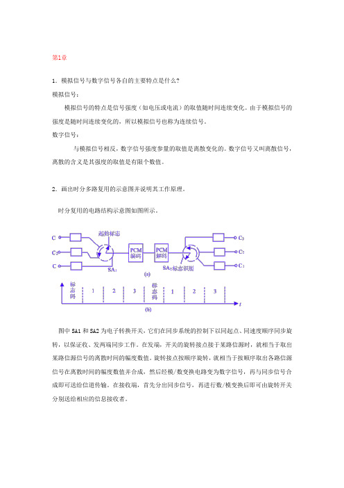
2.画出时分多路复用的示意图并说明其工作原理。
时分复用的电路结构示意图如图所示。
图中SA1和SA2为电子转换开关,它们在同步系统的控制下以同起点、同速度顺序同步旋转,以保证收、发两端同步工作。
在发端,开关的旋转接点接于某路信源时,就相当于取出某路信源信号的离散时间的幅度数值。
旋转接点按顺序旋转,就相当于按顺序取出各路信源信号在离散时间的幅度数值并合成,然后经模/数变换电路变为数字信号,再与同步信号合成即可送给信道传输。
在接收端,首先分出同步信号,再进行数/模变换后即可由旋转开关分别送给相应的信息接收者。
3.试述数字通信的主要特点。
(1)抗干扰能力强,无噪声积累(2)便于加密处理(3)利于采用时分复用实现多路通信(4)设备便于集成化、小型化(5) 占用频带宽4.简单说明数字通信系统有效性指标,可靠性指标各是什么?并说明其概念。
有效性指标(1)信息传输速率:信道的传输速率是以每秒钟所传输的信息量来衡量的。
信息传输速率的单位是比特/秒,或写成bit/s,即是每秒传输二进制码元的个数。
(2)符号传输速率符号传输速率也叫码元速率。
它是指单位时间内所传输码元的数目,其单位为“波特”(bd)。
(3)频带利用率频带利用率是指单位频带内的传输速率。
可靠性指标(1)误码率在传输过程中发生误码的码元个数与传输的总码元数之比。
(2)信号抖动在数字通信系统中,信号抖动是指数字信号码元相对于标准位置的随机偏移。
第2章1、假设某模拟信号的频谱如图1所示,试画出M s f f 2=时抽样信号的频谱。
答:2、某模拟信号的频谱如图2所示,设kHz f s 24=,试画出其抽样信号的频谱。
电子信息工程专业英语课文翻译(第3版)
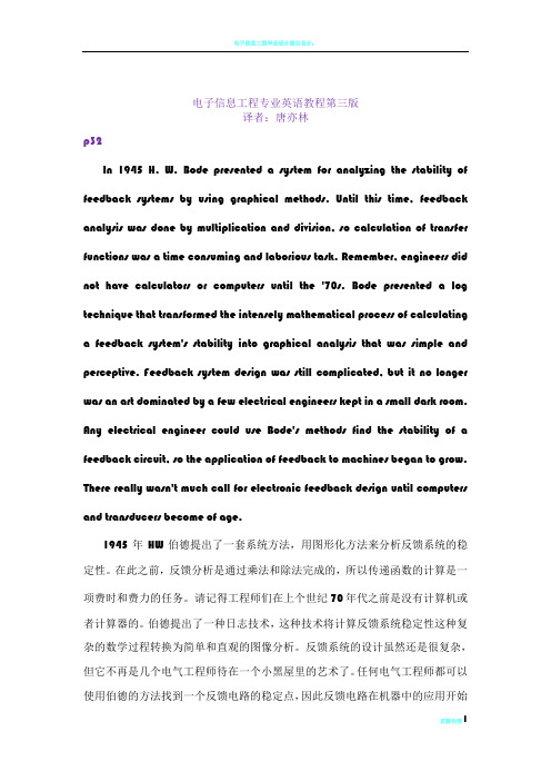
电子信息工程专业英语教程第三版译者:唐亦林p32In 1945 H. W. Bode presented a system for analyzing the stability of feedback systems by using graphical methods. Until this time, feedback analysis was done by multiplication and division, so calculation of transfer functions was a time consuming and laborious task. Remember, engineers did not have calculators or computers until the '70s. Bode presented a log technique that transformed the intensely mathematical process of calculating a feedback system's stability into graphical analysis that was simple and perceptive. Feedback system design was still complicated, but it no longer was an art dominated by a few electrical engineers kept in a small dark room. Any electrical engineer could use Bode's methods find the stability of a feedback circuit, so the application of feedback to machines began to grow. There really wasn't much call for electronic feedback design until computers and transducers become of age.1945年HW伯德提出了一套系统方法,用图形化方法来分析反馈系统的稳定性。
Reed_Solomon码的原理和软硬件实现
# $ %
# 所示。
图 #
二元域上的加法 责任编辑: 刘伯义
,H&!# , ! - H $1 20<1 H $1 I #
定稿日期: $""#!"%!#% 作者简介:
张 建 文 (#N?’! ) ,男,硕士研究生,主要研究方向为
作为 )- 码 作 为 一 种 循 环 码 有 与 之 对 应 的 生 成 多 项 式 ,
这样可以得到 ! (’ ) 。 /0 (!9( , 是 /0 (!&& , 的截短 #"( ) !$& ) 形式, 信 息 码 的 前 %" 位 都 是 !" ( ! ") 的零元素, 所以 ! (’ ) 只 需 要 是 #"()!9( 就 可 以 了 。 (! ) /0 编 码 的 硬 件 实 现 将信息码字用 /0 码 的 硬 件 实 现 是 根 据 循 环 码 的 特 点 , (% ) 多项式的形式表示成 ( 0 ’ )5 +%+#’%-#4+%+!’%-!4 … 4+9 用长除法, (’ ) 去除 ( . 0 ’) ’
逻辑电路 上来说就 异或如图 对 应 二 进 制 串 表 示 的 ##" 。 ( H ($ I (, #) ($ ) )- 码 的 生 成 多 项 式 和 生 成 矩 阵 是 线 性 循 环 码 的 一 种 。定 义 )- 码 是 一 种 多 元 456 码 , 在 !" (& ) 上, 纠 1 个 错 误 的 )- 码 的 参 数 如 下 码长 监督元数目 最小距离 (通 常 & 是 $ 的 幂 次 )
# # " # " $ " " # # % # " " #
- 1、下载文档前请自行甄别文档内容的完整性,平台不提供额外的编辑、内容补充、找答案等附加服务。
- 2、"仅部分预览"的文档,不可在线预览部分如存在完整性等问题,可反馈申请退款(可完整预览的文档不适用该条件!)。
- 3、如文档侵犯您的权益,请联系客服反馈,我们会尽快为您处理(人工客服工作时间:9:00-18:30)。
7th International Workshop on Algebraic and Combinatorial Coding Theory 18-24June2000,Bansko,Bulgaria pp.293-298 Soft-Decision Stack Decoding of Binary Reed-Muller Codes with“Look-Ahead”
Technique
Norbert Stolte,Ulrich Sorger
Institute for Communications Technology
Darmstadt University of Technology(TUD)
e-mail:stolte,uli@nesi.tu-darmstadt.de
Abstract
The performance of a stack algorithm to decode binary Reed-Muller codes is investigated.As metric to evaluate the different elements in the
stack we use a recently derived lower bound on the squared Euclidean
distance.It comprises a lower bound on the metric increase in future
decoding steps,similar to the-algorithm.Simulation results show that
in case of the code at a WER of with reasonable stack
size close to soft-decision ML-decoding performance can be achieved.
1Definitions
We assume BPSK transmission over an additive white Gaussian noise(AWGN) channel.The transmitted codeword denoted by
,,is corrupted by noise and at the receiver the real valued sequence is observed.
It is known[1][2]that the code of length can be composed using the-construction.I.e.with,
and
the obtained generalized concatenated(GC)code is the code.(see Fig.1)Since and are RM codes,they again can be viewed as GC codes and the same construction rule applies.This can be repeated several times and in this way the code is decomposed into
Fig.1:Decomposition of the code into two outer codes simple repetition codes,of different length,were is the dimension of the code.The codeword completely determines the codewords and vice versa.
Soft-decision bounded-minimum-distance(SD-BMD)decoding can be done by decoding only the outer codes and.We define the compo-nents of the soft-input vectors and of the codes and with and as
(1) and
(2) In[3]it was shown that if(1)and(2)are applied successively to calculate the soft-input values of the codes,the maximum-likelihood(ML) decoder decides for the codeword which minimizes the following sum
(3)
For a vector of estimates,, ,the sum
(4)
is a simple lower bound on the least value of(3)in the subcode
which is defined by
following inequality holds
(6) for.In that way similar to the-algorithm [4][5],the increase of in future decoding steps is lower bounded.
2Algorithm and Results
For decoding we use a stack algorithm in which the tree is searched in a breadth-first manner,that is all estimate vectors have same length.In-stead of performing full maximum-likelihood decoding tofind the in(6) a lower bound on is calculated.This is done using a second stack decoder with small stack which employs the metric given in(4). Whenever a stack overflow in the second stack occurs,the respective value of (4)of the element which is not kept in the stack gives a maximum value of
to be used in(6).Hence the metric to order the estimates in the main stack is given by
almost equal to the decoder with parameters.Moreover at a WER of quasi SDML-decoding performance can be achieved if the stack sizes are chosen to be and.
In Fig.4is shown the dependence of the WER on the signal to noise ratio for different stack sizes.At a WER of the performance degradation of the decoders with stack sizes and compared to SDML decoding is about0.4dB and0.2dB,respectively.Moreover compared to the“classical”-decoder the-decoder achieves an additional coding gain of3.4dB at WER=.
References
[1]F.J.MacWilliams,N.J.A.Sloane,”The Theory of Error-Correcting
Codes”,New York,North-Holland,2nd reprint,p.374,1983
[2]G.A.Kabatyansky,”On decoding Reed-Muller codes in semicontinuous
channel”,Proc.Second Int.Workshop Algebr.and Combin.Coding Theory, Leningrad,USSR,pp.87-91,1990
[3]N.Stolte,U.Sorger,G.Sessler,”Sequential Stack Decoding of Binary
Reed-Muller Codes”,ITG Fachbericht,3rd ITG Conference Source and Channel Coding,No.159,pp.63-69,2000
[4]Y.Han, C.Hartmann, C. C.Chen,”Efficient Priority-First Search
Maximum-Likelihood Soft-Decision Decoding of Linear Block Codes”, IEEE rm.Theory,V ol.IT-39,No.5,pp.1514-1523,1993 [5]N.Nilsson,”Principles of Artificial Intelligence”Berlin,Springer Verlag,
1982
Fig.3:Soft-decision decoding WER of the code,decoders with dif-ferent stack sizes
Fig.4:Soft-decision decoding WER of the code,decoders with dif-ferent stack sizes。