115-UniformSections subject to Bending

合集下载

NORSOKM-650 Rev.5 材料评定

4 4 5 5 5 5 5 5 7 8 8 8 8 8 8 8 8 8 9 9 9 9 9 9 10 10 10 10 10 10 12 12 13 14 15 15 15 17 20 20 20 20 21 22
3
4
5
6
7Leabharlann 8910Annex A (Informative) Manufacturing Summary front page and example
NORSOK standard M-650
Edition 4, September 2011
Foreword Introduction 1 2 Scope Normative and informative references 2.1 Normative references 2.2 Informative references Terms, definitions and abbreviations 3.1 Terms and definitions 3.2 Abbreviations Responsibilities 4.1 Purchasers responsibility 4.2 Manufacturers responsibility 4.3 Responsibilities of Qualifying Company Qualification of manufacturers 5.1 Basis for qualification of manufacturers 5.2 Evaluation for acceptance 5.3 Acceptance of qualification 5.4 Proof of acceptance Validity of qualification 6.1 Term of validity 6.2 Renewal of qualification 6.3 Transitional arrangements General requirements 7.1 Knowledge and relevant experience 7.2 Manufacturing facilities and equipment 7.3 Sub-contractors 7.4 Quality requirements for test laboratories and manufacturers of welded products Manufacturing Summary 8.1 Requirements for Manufacturing Summary 8.2 Content of the Manufacturing Summary Heat treatment 9.1 Heat treatment facilities and equipment 9.2 Heat treatment procedure 9.3 Verification of heat treatment procedure 10.1 10.2 10.3 10.4 11 11.1 11.2 11.3 Qualification of the manufacturing process Objective of qualification testing Essential variables Qualification testing Welding procedure qualifications Qualification test record (QTR) General Content of qualification test record (QTR) Required copies and distribution of qualification test record (QTR)

Effect of Stress Concentration on Magnetic Flux Leakage Signals from Blind-Hole Defects in Stressed

Res Nondestr Eval(1996)8:83–100©1996Springer-Verlag New York Inc.Effect of Stress Concentration on Magnetic Flux Leakage Signals from Blind-Hole Defects in Stressed Pipeline Steel T.W.Krause,R.W.Little,R.Barnes,R.M.Donaldson,B.Ma,and D.L.Atherton Department of Physics,Queen’s University,Kingston,Ontario,K7L3N6,CanadaAbstract.Stress-dependent magneticﬂux leakage(MFL)signals of the normal surface compo-nent(radial)MFL signal from blind-hole defects in pipeline steel were investigated.Three different stress rigs with uniaxial stress andﬁeld conﬁgurations were used.A double-peak feature in the MFL signal was deﬁned quantitatively by a saddle amplitude,which was taken as the difference between the average of the double peaks and the corresponding saddle point.Results indicated that the saddle amplitude increased linearly with increasing tensile surface stress and decreased, or did not exist,for increasing compressive surface stress.The stress-dependent saddle amplitude was shown to increase with increasing defect depth.Finite-element calculations indicated that stress concentration also increased with increasing defect depth.The measurements and analy-sis demonstrate that the stress-dependent saddle amplitude behavior in the radial MFL signal is associated with surface-stress concentrations near the blind-hole defects.IntroductionMagneticﬂux leakage(MFL)techniques are commonly used for the in-line inspection of pipelines for metal loss defects such as corrosion pits[1].The in-service operating pressures of gas pipelines generate large circumferential stresses that may reach70%of the yield strength of the pipe.These in-service stresses affect theﬂux leakage patterns and have been studied previously[2]–[7].In the presence of stress,defects act as“stress raisers”[8].Dependent upon the defect depth[9],the defects may generate stress con-centrations that exceed the yield strength in their vicinity.Stress raising around defects also may lead to enhanced stress corrosion cracking[10].There are two effects that may contribute to the generation of the stress-dependent MFL signal:1)the bulk effect of stress on the magnetic properties[11]–[16]and2)the effect of the defect as a stress raiser that is also dependent on the depth of the defect [9].Metal loss resulting from increasing defect depth increases the level of magnetic saturation in the vicinity of the defect and,therefore,increases the MFL signal.Similarly, by affecting the stress-dependent magnetic properties of the steel in the vicinity of the defect,the application of a bulk stress also affects the peak-to-peak MFL(MFL pp) signal.Stress concentrations in the vicinity of the defect have a similar effect.From a previous consideration[17],under a bending stress the two-dimensional solution for a100%through-wall defect or hole generates a peak stress level at the edge of the84Krause et al. hole that is2.4times that of the nominal background stress[8,17].Finite-element calculations and stress measurements[17]indicate that,for the same bending stress,the stress concentration for a round-bottomed pit that is50%of the through-wall thickness is1.2times the nominal stress.For a plate under uniform tensile stress,the maximum stress at the edge of a full cylindrical through-hole is three times that of the nominal stress [8,18].Stress concentrations occur at the two edges of the defect that are tangential to the applied stress direction.An increase in the pipe wallﬂux density typically results in an increase in the MFL signal due to increased saturation of the steel in the defect region.The effect of stress on the MFL pp signal has been shown to increase for increasingﬂux densities in the range of 0.65to1.24T[9,13]–[16].It is expected,therefore,that stress concentration combined with increasingﬂux density may similarly affect the MFL signal.Observations of a double-peak feature that increases in amplitude with increasing applied tensile stress have been made for normal-surface component(radial)MFL signals for various uniaxial orientations of stress andﬁeld applied to pipeline steel[5,11].In particular,the amplitude of the double-peak feature(hereafter referred to as the saddle amplitude)has been observed to increase linearly with increasing levels of applied stress and has been associated with stress patterns around the defect itself[12,14].In this paper we provide evidence that strongly supports this claim.Further,it is demonstrated that the double-peak feature in the MFL signal may be associated primarily with stress concentrations that appear in the vicinity of the defect near the surface of the steel pipeline sample,and also that the stress concentration and resultant saddle amplitude in the MFL signal increase with increasing defect depth.Experimental ApparatusThe experimental apparatus is described in detail elsewhere[11,12].The apparatus used to measure the radial component of theﬂux leakageﬁeld from a defect on the same side of the sample as the measuring apparatus(near side)consisted of a Hall probe,an ampliﬁer to amplify the Hall signal,and a computer for data acquisition.The radialﬂux leakage signal was measured at scanned positions set at1-mm intervals(0.5mm for the semicircular pipe section)across the area of the defect.The radialﬂux leakage signal was taken as the average of100measurements taken at each position.Pipeline Sample and Stressing ApparatusSamples of pipeline steel used in this study were cut from a610-mm(24-in.)diameter X70steel pipe of9-mm wall thickness.Theﬁrst sample used was a102-mm(4-in.)wide semicircular section cut in the pipe hoop direction.Other samples used were4.27-m long axial strips that were also102mm(4in.)wide.The pipeline steel composition is given elsewhere[17].There were three separate experimental test rigs.Theﬁrst apparatus is the semi-circular hoop bending rig shown in Fig.1.The second and third apparatus use the single-strip beam-bending arrangement and the composite beam-bending arrangement,Magnetic Flux Leakage Signals from Blind-Hole Defects85Fig.1.The semicircular pipe section and bending stress rig for the production of surface stress in semicircular sections of pipe steel.both described elsewhere[11,12].Surface stresses up to±300MPa were applied using the three stress rigs.This is below the yield stress of the pipe steel,which is at500MPa. All three sets of apparatus have a13-mm diameter ball-milled external pit machined to50%of the steel wall thickness.The composite beam apparatus also has two more 13-mm diameter ball-milled external pits machined to depths of25and75%.An area of about40mm by40mm around the defect was stripped of its epoxy coating to expose the pipe steel.The defect area was magnetized to a maximum axialﬂux density of1.6T using ferrite magnets.For the semicircular pipe section,steel hingedﬁngers were used to couple theﬂux from the magnets into the steel pipe,while for the two beams,steel brushes shaped to the curvature of the beams coupledﬂux into the steel samples. Semicircular Pipe Section Stress RigIn theﬁrst stress rig,shown in Fig.1,a semicircular pipe section is held stationary by a ﬁxed clamp,while the other is connected to a movable clamp.The movable clamp is free to travel along a horizontal threaded rod as the rod is rotated with the handle,the result being the application of a hoop-bending stress.When the clamp is moved inward,tension is created on the outside and compression on the inside pipe surface,with the opposite being true if the clamp were to be moved outward.A“clamp position versus stress”calibration was obtained theoretically[17]and veriﬁed using strain gauges(placed well away from the defect region).86Krause et al. Single BeamThe single-strip beam is a102-mm wide strip of steel cut in the axial direction from the 610-mm diameter pipe with a thickness of9mm and a length of4.27m.The low rigidity of the single beam allows bending by simply hanging masses of about5kg from one end of the beam or supporting it at a raised height while the middle length of the beam is supported and the opposite end of the beam isﬁxed in position.Composite BeamThe third apparatus utilizes a composite beam and an arrangement to bend the beam [11,12].The composite beam is made from two axial strips of pipeline steel that are separated at aﬁxed distance of29mm by an alternatingﬁberglass–wood composite. The composite materials are bonded together with high-strength epoxy resin.Under a bending stress the neutral axis of the beam is outside the pipeline steel regions,so that nearly uniform stress is generated through the thickness of the steel walls.Because the composite beam is much more rigid,the beam is stressed by placing it parallel to a comparably rigid pipe section of equal length separated by a wood saddle in the middle. At one end the beam and pipe are held together by a clamp or chain,and at the other end the beam and pipe are pulled together by another clamp with a scissor jack.For tests using tensile stress the steel strip with the defect in it is on the side facing away from the rigid pipe,with the composite beam above the pipe.For compressive stress the steel strip is on the side facing toward the pipe and with the beam underneath the pipe,so that the detector can be placed on top of the beam.Stress CyclesThree different procedures of applyingﬁeld and stress are used to perform the mea-surements:1)the“normal cycle,”which involves magnetizing the beam with no applied stress and maintaining the appliedﬁeld during the stressing of the beam;2)the“opposite cycle,”which is similar to the“normal cycle”except that the magnetization is generated with theﬁeld in the opposite polarity;and3)the“after-cycle,”which involves removing the magnet before each stressing increment and then replacing it so that the beam is remagnetized after each change of stress.In all three methods,the defects are scanned at ﬁxed levels of stress.Of the three cycles,the after-cycle is the most similar to an actual pipeline pigging measurement.Measurements of the peak-to-peak magneticﬂux leakage(MFL pp)signal in the normal-cycle mode across a50%penetration round-bottomed blind-hole–simulated de-fect for various levels of applied tensile and compressive stress in the semicircular pipe section were performed using the hoop-bending stress rig shown in Fig.1.Starting from0MPa,tensile stress up to250MPa was applied followed by changes in stress to 250MPa compressive stress and,ﬁnally,back to a0-MPa stress level.The MFL signal was recorded at various levels of applied stress.The stress in the pipe section was ad-justed by varying the distance between the ends of the semicircular pipe section in the stress rig to various strain gauge calibrated settings.Magnetic Flux Leakage Signals from Blind-Hole Defects87 For the composite beam tensile stress scans were performed,ﬁrst for all three defects and stress cycles,and then followed by compressive stress scans,since a reorientation of the beam was required.No compressive stress scans were performed for the single beam.Variation of Pipeline Steel Flux DensityThe totalﬂux density within the semicircular pipe section was measured by removing the magnetizing system,noting theﬂux change,reversing the polarity of the magnetizer, applying it again,and noting theﬂux change again.The average of the twoﬂux readings was taken and theﬂux density within the pipe and was found to be1.54T.The totalﬂux density within the single-beam stress rig was determined in the same manner and was found to be1.6T.Two techniques were used to vary theﬂux density within the composite beam pipe wall and are described in detail elsewhere[9,13].Theﬁrst technique consisted of changing the size of the magnets used,and the second involved the application of partial shorting bars.The steel bars diverted some of theﬂux from the magnets and therefore reduced theﬂux density in the pipe wall.An integrating voltageﬂuxmeter,connected to a13-turn coil wound around one section of steel beam and through a hole in the center of the composite beam assembly,was used to determine theﬂux density within the pipe wall. The four pipe wallﬂux densities generated within the composite beam pipe wall using these two techniques were0.65T,0.84T,1.03T,and1.24T.AnalysisThe peak-to-peak radial component of the magneticﬂux leakage(MFL pp)signal is ob-tained by taking the difference between the maximum(positive)and minimum(negative) components of the MFL signal.Positive saddle amplitude values are obtained from the MFL signal by evaluating the difference between the average of the two positive peaks and the positive saddle point.Negative saddle amplitude values are obtained in the same manner,except that the negative double MFL peaks and the negative saddle point are used for the evaluation.Both the variation of the MFL pp signal and the saddle amplitude as functions of stress were investigated.Finite-Element CalculationsA three-dimensionalﬁnite-element method was used to model the stress pattern surround-ing the defect.Finite-element modeling was performed using the ANSYS Revision4.4 by Swanson Analysis Systems.A ten-node tetrahedral element with three directional degrees of freedom at each node was used to mesh the solid model.The volumes were deﬁned using a solid modeling approach,where the geometry of the object was described by specifying key points,lines,areas,and volumes.ANSYS thenﬁlled in the solid model with nodes and elements based on the user-deﬁned element shape and size.88Krause et al.Fig.2.(a)Surface and contour plots of the radial magneticﬂux leakage from the near side of a13-mm-diameter ball-milled50%defect in the semicircular pipe section under a tensile stress of250MPa during a normal cycle.Theﬁnite-element calculations modeled aﬂat plate with a ball-milled defect.The plate dimensions were taken as50mm×50mm with a thickness of9mm,which was the same as that of the pipeline steel samples.The radius of curvature of the ball-mill that generated the defect was taken as6.35mm.The full defect radius was,therefore,only attained at71%defect depth.This may have affected the calculations since the defect radius was changing continuously with respect to the mesh distribution up to71%of the wall thickness.Young’s modulus was taken as210GPa and Poisson’s ratio as0.28. Calculations were performed for a nominal stress of190MPa.ResultsSemicircular Pipe Section:MFL pp MeasurementsFigures2a and2b show surface and contour plots of the radial magneticﬂux density leakageﬁeld over the defect for tensile and compressive stresses of250MPa,respectively. Both scans are from the normal-cycle procedure using constant magnetization.The amplitude of a signal is obtained by taking the difference between the maximum andMagnetic Flux Leakage Signals from Blind-Hole Defects89Fig.2.(b)Surface and contour plots of the radial magneticﬂux leakage from the near side of a13-mm-diameter ball-milled pit in the semicircular pipe section under compressive stress at250MPa during a normal cycle.minimum values ofﬂux density over the area of the scan(MFL pp).The proﬁle of the contours is typical for all scans,with slight variations with changing paring the two scans,a more pronounced double-peak feature is observed for the tensile surface stress case than for the compressive surface stress case.The MFL pp signal as a function of stress for the semicircular pipe section under bending-hoop stress is shown in Fig.3.Starting at0MPa,the variation of the MFL pp signal with surface stress demonstrates an initial increase with the application of tensile stress followed by a decrease and a large hysteresis loop as the stress is cycled from 250MPa to−250MPa.Under a compressive stress the variation of the MFL pp signal is smaller,as is the hysteresis.Theﬁnal zero-stress MFL pp signal is greater than the initial starting point.Arrows indicate the order in which the data were taken.Variation of Saddle Amplitude with StressResults obtained from an analysis of the positive and negative saddle amplitudes as a function of surface stress in the normal cycle are shown for the semicircular pipe section in Fig.4.Positive and negative saddle amplitudes are present for the zero-stress case.90Krause et al.Fig.3.Peak-to-peak MFL signal from the near side as a function of surface stress in the normal cycle for a13-mm-diameter ball-milled50%defect on the semicircular pipe section under hoop-bending stress with an applied pipe wallﬂux density of1.54Tesla at0MPa.Since hysteresis is present,arrows indicate the direction in which the data were taken.The positive saddle amplitude increases linearly from a minimum at250MPa compressive stress to a maximum at200MPa tensile stress.Some hystersis is evident.In comparison, the negative saddle amplitude is smaller in magnitude,more hysteretic,and slightly less linear.For the single-beam stress rig,observations of a saddle amplitude that depended linearly on stress were made for there tensile surface stress measurements equal to and greater than200MPa measured in the normal cycle.In this rig a saddle was not observed for zero or applied compressive stresses.As in the semicircular pipe section,the magnitude of the positive saddle amplitudes was greater than the corresponding negative saddle amplitudes.The variations of the positive and negative saddle amplitudes with stress for the composite beam for the three defect depths in the normal cycle at1.24T are shown in Fig.5for tensile stress values.For the composite beam no saddle was observed for any zero or compressive stress values,which is in contrast to the semicircular pipe section where a saddle amplitude that was a decreasing function of increasing compressive stress was observed.This result is considered further in the discussion.The results for the composite beam indicate an increasing variation of saddle amplitude with stress forMagnetic Flux Leakage Signals from Blind-Hole Defects91Fig.4.Positive(•)and negative( )saddle amplitudes as functions of surface stress using the semi-circular pipeline apparatus with aﬁeld of1.54T during the normal cycle are plotted for the13-mm ball-milled50%defect.increasing defect depth.For the25and50%depth defects the positive saddle amplitudes are greater in magnitude than the negative saddle amplitude values for equivalent levels of stress,while at75%this difference is not as great.The dependence of the positive and negative saddle amplitudes upon stress in the composite beam for the three different defect depths for measurements performed in the after-cycle at1.24T are shown in Fig.6.In contrast to the normal-cycle measurements for the25and50%defects,the magnitude of the negative saddle amplitudes is greater than that of the positive saddle amplitudes,while there is no observed difference between the magnitudes for the75%defect.The rate of change of the saddle amplitude with stress is greatest for the75%defect and least for the25%defect.Stress-Dependent Saddle Amplitude SlopesLinear bestﬁts were applied to the saddle amplitude data as a function of stress for the three different stress rigs.The slopes of saddle amplitude variation with stress for the normal cycle in the three different stress rigs are shown in Table1.Several observations can be made for the normal-cycle stress applied in the three different stress rigs.These92Krause et al.Fig.5.Saddle amplitudes as a function of stress in the composite beam apparatus from13-mm ball-milled defects in aﬁeld of1.24T in the normal cycle are plotted for the25%defect for the positive( ) and negative( ),for the50%defect for the positive( )and negative( ),and for the75%defect for the positive( )and negative(•)saddle amplitudes.Table1.Bestﬁt slopes for normal-cycle MFL pp and saddle amplitude with different defect depths in the composite beam and50%defect in the semicircular pipe section and single beam.%MFL pp vs.Stress-dependent Stress-dependent+Sad.amp.−Sad.amp. Defect stress slope saddle amplitude saddle amplitude MFL pp slope MFL pp slope depth(10−12T/Pa)pos.(10−13T/Pa)neg.(10−13T/Pa)(=col.3/col.2)(=col.4/col.2) Composite Beam(B=1.24T)25% 1.6210.130.0650% 5.1760.140.1275%11.019.119.50.1740.177 Semicircular Pipe Section(B=1.54T)50%—118——Single Beam(B=1.6T)50% 2.3 1.68±39±30.350.43Fig.6.Saddle amplitudes as a function of stress in the composite beam apparatus from13-mm ball-milled defects in aﬁeld of1.24T in the after-cycle are plotted for the25%defect for the positive( ) and negative( ),for the50%defect for the positive( )and negative( ),and for the75%defect for the positive( )and negative(•)saddle amplitudes.are:1)the slope directions of the positive and negative saddles as a function of stress are all positive;2)the rate of change of saddle amplitude as a function of stress for all three stress rigs is of the same order of magnitude,in contrast to the MFL pp signal variations with stress,which demonstrate little correlation between the three different stress rigs: 3)the magnitude of the saddle amplitudes obtained from the positive saddle curves is greater than the corresponding negative saddle curves in the normal cycle;4)no change in the saddle amplitudes was observed under compressive stress for bending stress applied in the axial direction in both the single and composite beams;5)the magnitudes of the saddle amplitudes for the semicircular pipe section are approximately four times greater than those observed for the single and composite beams,and do not go to zero even with the largest application of compressive stress;and6)there is a general increase in the positive and negative saddle amplitude slopes with increasing defect depth.The slopes obtained from the after-cycle and opposite-cycle also demonstrate an increasing saddle amplitude slope with increasing defect depth,although increased in-tercepts for the25and50%defects for the negative saddle amplitude variation are observed.This increase can be seen for the after-cycle in a comparison of Figs.5and6. The sum of the positive and negative saddle amplitude slopes(the total saddle amplitudeFig.7.The sum of positive and negative saddle amplitude stress slopes plotted as a function of% defect depth for the normal cycle( ),after-cycle,( )and opposite cycle( )in the composite beam (B=1.24T).The solid and dashed curves are lines to guide the eye.slope)obtained from the three stress cycle results are plotted as a function of percent defect depth in Fig.7.The total saddle amplitude slope is plotted as a function ofﬂux density for the after-cycle in Fig.8.For all three cycles the results indicated an increasing total saddle am-plitude with increasingﬂux density.The stress concentration factor is a constant for constant defect depth and,therefore, may be related to the slope of the saddle amplitude variation with stress.However,for the zero-stress case,the radialﬂux leakage signal demonstrates a considerable increase with increasing defect depth[19,20].Therefore,to perform a comparison of the variation of the saddle amplitude with stress for different defect depths with calculated values of the stress concentration,it is necessary to normalize the stress-dependent saddle amplitude slopes by their respective zero-stress MFL pp signals.A comparison of the normalized saddle amplitude slopes with the maximum and surface maximum stress concentrations obtained fromﬁnite-element calculations is shown in Fig.9.The stress-dependent saddle amplitude slopes have been averaged over the three cycles,normalized by their respective zero stress MFL pp signals,and scaled to the calculated maximum surface stress at75% defect depth.The normalized and scaled saddle amplitude slopes have beenﬁtted in Fig.9with anFig.8.Sum of positive and negative saddle amplitude stress slopes plotted as a function of pipe wall ﬂux density for the after-cycle( )in the composite beam(B=1.24T).The solid curve is simply a line to guide the eye.empirical formulation given byA=a sinh(bD),(1)where A is the sum of the positive and negative saddle amplitude slopes,D is the percent defect depth,and a and b areﬁtting parameters given by(a,b)=(0.71,0.018). Equation(1)holds in the limit of a0%defect since the total saddle amplitude A goes to zero as the MFL pp signal goes to zero.Theﬁnite-element calculations indicate that both the maximum and surface maximum stress concentration are increasing functions of percent defect depth.Starting at0%defect depth,the maximum stress concentration increases more rapidly than both the surface maximum and the normalized and scaled saddle amplitude slope values.Slower increases in theﬁnite-element calculations are observed in the vicinity of70%,which corresponds with the defect depth in theﬁnite-element model where the radius of the defect reaches its maximum of6.35mm.After90%the surface maximum concentration becomes the maximum stress concentration.The hyperbolic sine function,Eq.(1),coincides with the ﬁnite-element calculations above75%defect depth and with the theoretical fractional change in stress concentration at100%defect depth.Fig.9.Normalized change in maximum stress( )and maximum surface stress(⊕)as a function of%defect depth as obtained fromﬁnite-element calculations.The total saddle amplitude stress slopes ( )for the composite beam normalized by their respective zero-stress MFL pp signals and averaged over the three different stress cycles have been scaled to the maximum surface stress(SurfaceσMAX)ﬁnite-element calculations at75%defect depth.The dashed lines are spline curves through the pointsobtained from theﬁnite-element calculations and the solid line is a bestﬁt of the empirical relation,Eq.(1).DiscussionSemicircular Pipe Section:MFL pp MeasurementsThe application of a bending stress in the semicircular pipe section complicates the prediction of the magneticﬂux leakage stress behavior of the pipe since,if the upper surface of the pipe with the near-side defect is under tensile stress,then the inner surface will be under compressive stress.A further complication in this system is the direction of the magnetic easy axis with respect to the direction of the applied stress.The magnetic easy axis is at90◦to the direction of the applied stress,and,therefore,the magnetic properties of the pipeline steel are different[21]from those where the stress and easy axis are aligned in the same direction[22].Geometric properties of the semicircular pipe stress rig also may play a role in affecting the stress-dependent variation of the MFL pp signal,since the radius of curvature and therefore the length of theﬂux path in the semicircular pipe section changes as a function of stress with respect to theﬁxed length of the magnetizer.Furthermore,different levels of pipe wallﬂux density at equivalent stress levels for increasing and decreasing applied stresses may arise because of hystereticﬂux coupling in the hingedﬁnger–semicircular stress system.This may explain the severe hysteresis observed in the radial MFL pp signal for the semicircular pipe section under tensile stress shown in Fig.3.The application of a hoop-bending stress that is either tensile or compressive results in an overall decrease of the MFL pp signal for either surface tensile or surface compressive applied stress.However,there is an initial increase of the MFL pp signal under a surface tensile stress of50MPa.This may be attributed to the presence of a residual compres-sive surface stress present within the pipe.This suggestion is supported by spring-back measurements observed when the pipe section was cut in half[22].Stress-Dependent Saddle Amplitude:Stress Concentration FactorsThe variation of the MFL pp signal with stress appears to be associated primarily with the bulk effects of stress[9],[11]–[13]and pipe wallﬂux density[9,13]on the magnetic properties of steel in the general vicinity of the defect.However,we propose that the double-peak feature in the MFL pp signal and the variation of the saddle amplitude with stress is associated with the near-surface variation of stress in the immediate vicinity of the defect,which acts as a local stress raiser[17].Measurements of the MFL pp signal with almost uniform bulk stress in the composite beam stress rig indicate an increase of the MFL pp signal with increasing uniaxial tensile stress[9,13].Similarly,the variation of the saddle amplitude as a function of stress at the near-side surface of the defect demonstrated the same positive dependence.The rate of change of the saddle amplitude as a function of stress was also of the same order of magnitude in all three apparatus.Since it is the surface stress in all three apparatus that is monitored,we associate the saddle amplitude behavior as a function of stress with the corresponding variation of surface stress in the pipeline steel in the vicinity of the defect.Normalization of the stress-dependent saddle amplitude variation by the stress-de-pendent MFL pp slope for the case of the composite beam is shown in Table1.The results indicate that the saddle amplitude increases with defect depth faster than the stress-dependent MFL pp signal.Also shown in Table1are the positive and negative saddle amplitude slopes for the single beam normalized by the stress-dependent MFL pp slope for the50%defect.The values for the normalized saddle amplitude slopes obtained in this manner are more than twice those obtained for the50%defect in the composite beam. Normalization of the semicircular pipe section stress-dependent saddle amplitude by the corresponding MFL pp stress-dependent signal generates a nonlinear stress variation since the MFL pp signal varies nonlinearly over the applied tension–compression stress cycle.As was shown elsewhere[9,13],the single and composite beams demonstrate a compressive stress dependence,while no saddle amplitude is observed in this applied stress region.These results demonstrate that the variation of the MFL pp signal as a function of the bulk stress effect cannot explain the observed stress-dependent variation of the saddle amplitude.Furthermore,the slope of the saddle amplitude as a function of measured surface stress for the50%defect in the three different stress rigs,two of which are under a bending surface stress,are all of the same order.These points indicate。

fulltext(3)

As a result of the fast development of new materials, urged by the demand of more durable and resistant materials, fibre reinforced plastic composites (FRP) were introduced as replacement for the reinforcing steel. Carbon FRP has been used since the seventies in the space industry, where the requirement for lightweight, high-tensile strength, corrosion and high temperature resistance is essential. Recently, in Brazil and many other countries, FILl) composites (mainly carbon) have been used in strengthening slabs (of bridges and parking floors), beams (of
Materials and Structures/Mat~riaux et Constructions,Vol.35, Januanj-February 2002, pp 50-58
Strength of short concrete columns confined with CFRP sheets
I
1. I N T R O D U C T I O N
External confinement has been successfully applied to concrete columns in order to increase their strength and ductility or to recover them from eventual deterioration originated from different sources. In early constructions, concrete-filled steel tubes were used for some of the reasons mentioned above. The main disadvantages of this technique are the high cost for maintenance against corrosion, the low fire resistance and the heavy weight of the tubes. 1359-5997/02 9 R.ILEM 50

ASTM C158

Designation:C 158–02Standard Test Methods forStrength of Glass by Flexure (Determination of Modulus of Rupture)1This standard is issued under the ﬁxed designation C 158;the number immediately following the designation indicates the year of original adoption or,in the case of revision,the year of last revision.A number in parentheses indicates the year of last reapproval.A superscript epsilon (e )indicates an editorial change since the last revision or reapproval.1.Scope1.1These test methods cover the determination of the modulus of rupture in bending of glass and glass-ceramics.1.2These test methods are applicable to annealed and prestressed glasses and glass-ceramics available in varied forms.Alternative test methods are described;the test method used shall be determined by the purpose of the test and geometric characteristics of specimens representative of the material.1.2.1Test Method A is a test for modulus of rupture of ﬂat glass.1.2.2Test Method B is a comparative test for modulus of rupture of glass and glass-ceramics.1.3The test methods appear in the following order:Sections Test Method A Test Method B6to 910to 151.4This standard does not purport to address all of the safety concerns,if any,associated with its use.It is the responsibility of the user of this standard to establish appro-priate safety and health practices and determine the applica-bility of regulatory limitations prior to use.Speciﬁc hazard statements are given in Section 10and A1.5,A2.3.3,A2.4.3and A2.5.3.2.Referenced Documents 2.1ASTM Standards:C 148Test Methods for Polariscopic Examination of Glass Containers 2E 4Practices for Force Veriﬁcation of Testing Machines 3E 380Practice for Use of the International System of Units (SI)(the Modernized Metric System)43.Terminology 3.1Deﬁnitions:3.1.1glass-ceramics —solid materials,predominantly crys-talline in nature,formed by the controlled crystallization of glasses.3.1.2modulus of rupture in bending —the value of maxi-mum tensile or compressive stress (whichever causes failure)in the extreme ﬁber of a beam loaded to failure in bending computed from the ﬂexure formula:S b 5M c I(1)where:M =maximum bending moment,computed from themaximum load and the original moment arm,c =initial distance from the neutral axis to the extremeﬁber where failure occurs,andI =initial moment of inertia of the cross section about theneutral axis.3.1.3prestressed —material in which a signiﬁcant and con-trolled degree of compressive stress has been deliberately produced in the surfaces.3.1.4standard laboratory atmosphere —an atmosphere hav-ing a temperature of 2362°C and a relative humidity of 40610%.3.2Deﬁnitions of Terms Speciﬁc to This Standard:3.2.1abraded —describes a test specimen that has at least a portion of the area of maximum surface tensile stress subjected to an operationally deﬁned procedure for mechanical abrasion.The severity and uniformity of abrasion should be sufficient to ensure origin of failure substantially in the region of maximum stress.3.2.2annealed glass —describes a specimen that shall not have a temper or degree of residual stress resulting from prior thermal treatment in excess of the following limits when measured polarimetrically (see Annex A1):3.2.2.1Specimens of rectangular section shall not have a tensile stress at the midplane of more than 1.38-MPa (200-psi)nor more than 2.76-MPa (400-psi)compression at the surface.3.2.2.2Specimens in rod form may be examined by viewing through a diameter at least four diameters from an end.The apparent central axial tension shall not exceed 0.92MPa (133psi).Surface compression,if measured on sections cut from the rods,shall not exceed 2.76MPa (400psi)when viewed axially.1These test methods are under the jurisdiction of ASTM Committee C14on Glass and Glass Products and are the direct responsibility of Subcommittee C14.04on Physical and Mechanical Properties.Current edition approved Oct.10,2002.Published October 2002.Originally published as C 158–st previous edition C 158–95(2000).2Annual Book of ASTM Standards ,V ol 15.02.3Annual Book of ASTM Standards ,V ol 03.01.4Annual Book of ASTM Standards ,V ol 14.04.1Copyright ©ASTM International,100Barr Harbor Drive,PO Box C700,West Conshohocken,PA 19428-2959,United States.Copyright ASTM InternationalProvided by IHS under license with ASTMNot for ResaleNo reproduction or networking permitted without license from IHS--`-`-`,,`,,`,`,,`---4.Signiﬁcance and Use4.1For the purpose of this test,glasses and glass-ceramics are considered brittle (perfectly elastic)and to have the property that fracture normally occurs at the surface of the test specimen from the principal tensile stress.The modulus of rupture is considered a valid measure of the tensile strength subject to the considerations discussed below.4.2It is recognized that the modulus of rupture for a group of test specimens is inﬂuenced by variables associated with the test procedure.These include the rate of stressing,test envi-ronment,and the area of the specimen subjected to stress.Such factors are speciﬁed in the test procedure or required to be stated in the report.4.3It is also recognized that the variables having the greatest effect on the modulus of rupture value for a group of test specimens are the condition of the surfaces and glass quality near the surfaces in regard to the number and severity of stress-concentrating discontinuities or ﬂaws,and the degree of prestress existing in the specimens.Each of these can represent an inherent part of the strength characteristic being determined or can be a random interfering factor in the measurement.4.4Test Method A is designed to include the condition of the surface of the specimen as a factor in the measured strength.It is,therefore,desirable to subject a ﬁxed and signiﬁcant area of the surface to the maximum tensile stress.Since the number and severity of surface ﬂaws in glass are primarily determined by manufacturing and handling pro-cesses,this test method is limited to products from which specimens of suitable size can be obtained with minimal dependence of measured strength upon specimen preparation techniques.This test method is therefore designated as a test for modulus of rupture of ﬂat glass.4.5Test Method B describes a general procedure for test,applicable to specimens of rectangular or elliptical cross section.This test method is based on the assumption that a comparative measurement of strength on groups of specimens is of signiﬁcance for many purposes,such as determining the effect of environment or stress duration,or the effectiveness of varied prestressing techniques or strengths characteristic of glass-ceramics of differing composition or heat treatment.In this test method the surfaces of the specimens are not assumedto be characteristic of a product or material,but areconsidered to be determined by the procedures used to prepare the specimens.Though the stated procedure permits a wide varia-tion in both specimen size and test geometry,it is necessary to use identical test conditions and equivalent procedures for specimen preparation to obtain comparable strength values.The use of a controlled abrasion of the specimen as a ﬁnal normalizing procedure is recommended for such comparative tests.4.6A comparative abraded strength,determined as sug-gested in Test Method B,is not to be considered as a minimum value characteristic of the material tested nor as directly related to a maximum attainable strength value through test of specimens with identical ﬂaws.The operationally deﬁned abrasion procedure undoubtedly produces ﬂaws of differing severity when applied to varied materials,and the measured comparative strengths describe the relative ability to withstand externally induced stress as affected by the speciﬁc abrasion procedure.5.Apparatus5.1Testing Machine —The loading mechanism shall be sufficiently adjustable to give the required uniform rate of increase of stress.The load-measuring system shall be essen-tially free of inertial lag at the loading rates used and shall be equipped with means for retaining indication of the maximum load applied to the specimen.The accuracy of the testing machine shall conform to the requirements of Practice E 4.5.2Bearing Edges —Cylindrical bearing edges of approxi-mately 3-mm (1⁄8-in.)radius shall be used for the support of the test specimen and the application of the load.The bearing edges shall be of steel and sufficiently hardened to prevent excessive deformation under load.Two-point loading tests shall be performed with the loading member pivoted about a central transverse axis to ensure equal distribution of load between the two bearing edges.For the testing of specimens of rectangular section,both loading bearing edges and one sup-port bearing edge also shall be provided laterally to compen-sate for irregularities of the test specimen.Fig.1shows a suitable arrangement using pinned bearing edges.In test of specimens of a circular or elliptical section,the ﬁxed cylindri-cal support edges may have a curvature of approximately 76FIG.1Pinned Bearing Edgesmm (3in.)in the plane of the bearing edge to stabilize the alignment of the specimens.Such support edges are shown in Fig.2.TEST METHOD A—TEST FOR MODULUS OFRUPTURE OF FLAT GLASS 6.Test Specimens6.1Preparation of Specimens —Test specimens shall be cut from the sheet stock with a diamond or a cutting wheel.Both longitudinal cuts shall be on the same original surface and none of the original edge of the sheet shall be used as a longitudinal side of the specimen.End cuts may be on either surface.The direction of cutting of half of the total number of specimens shall be perpendicular to the direction of cutting of the remainder.Specimens that must be cut from sheet stock prior to the use of a prestressing treatment shall have the corners of the longitudinal edges rounded to minimize damage to the edges in the prestressing process.All operations shall be performed with the direction of grind or polish parallel to the longitudinal axis.The radius of the corner shall not exceed 1.6mm (1⁄16in.).6.2Size of Specimens —The specimens shall be approxi-mately 250mm (10in.)in length and 38.163.2mm (11⁄261⁄8in.)in width.The variation in width or thickness shall not exceed 5%from one end to the other.6.3Number of Specimens —At least 30specimens shall be used for one test and shall preferably be taken from several sheets,or regions of a single sheet.6.4Examination of Specimens —Any specimen may be rejected prior to test for observable defects considered likely to affect the modulus of rupture.To be considered representative of annealed glass the specimens must meet the requirement of 3.2.2.At least 30%of the specimens shall be examined for residual stress.If any of these fail to meet the requirement,the remainder of the specimens shall be examined and those exceeding the stated limit shall be rejected.6.5Float Glass —The surface of ﬂoat glass in contact with tin has been found to be lower in strength (7)as compared to the “air”surface.For comparative tests,therefore,surface orientation should be kept constant.7.Procedure7.1Space the supporting edges of the test ﬁxture 200mm(8.00in.)apart and centrally position the loading edges with a separation of 100mm (4.00in.).Break specimens having cut edges with the cutter marks on the face under compression.Carefully place each specimen in the test ﬁxture to minimize possible damage and to ensure alignment of specimen in the ﬁxture.The permissible maximum ﬁber stress due to initial load on the specimen shall not exceed 25%of the mean modulus of rupture.Load the specimen at a constant rate to failure.For annealed glass the rate of loading shall correspond to a rate of increase of maximum stress of 1.160.2MPa/s (1000062000psi/min).Test prestressed glasses with the increase of maximum stress per minute between 80and 120%of the modulus of rupture.The ﬁrst six specimens of the group may be tested at a loading rate based on an estimate of the modulus of rupture and the average value for these specimens used to correct this estimate.If range of width and thickness variation in the specimens is less than 5%,the mean values may be used to represent all specimens for the purpose of calculation of rate of loading.7.2Determine the thickness and width of each specimen to 61%.To avoid damage from gaging in the critical area,take measurements prior to testing near each end with a separation equal to the support span,and average the values.Measure-ments following test shall be in the uniformly stressed region of the specimen.7.3Determine the location of point of failure and note it as edge or face origin.Plastic or other tape of low elastic modulus 5may be used on the compressive surface to contain the fragmentation and allow observation of point of failure for highly prestressed specimens.Report all values,although segregation of edge break values is permitted.8.Calculation8.1Calculate the modulus of rupture,initial maximum ﬁber stress,and rate of increase of stress as follows:5Scotch Brand plastic tape,Catalog No.191-A,manufactured by 3M Co.,3M Center,St.Paul,MN 55144,has been found suitable for this purpose.FIG.2Fixed Cylindrical Support Edges8.1.1Modulus of rupture:S53Labd2(2)8.1.2Maximum stress due to initial load if present:S053L0abd(3)8.1.3Rate of increase of maximum stress:R53abd23D LD t(4)R5S2S0 twhere:S=modulus of rupture,MPa(psi),S0=maximumﬁber stress due to initial load if present,MPa(psi),R=rate of increase of maximumﬁber stress,MPa/s (psi/min),L=breaking load including initial load,N(lbf),L0=initial load,N(lbf),a=moment arm or distance between adjacent sup-port and loading edges,mm(in.),b=width of specimen,mm(in.),d=thickness of specimen,mm(in.),t=time from start of continuous loading to rupture, s(min),andD L/D t=rate of increase of load,N/s(lbf/min).9.Report9.1Report the following:9.1.1Test method used,9.1.2Identiﬁcation of the glass tested,including any special treatment(for specimens derived from manufacturing pro-cesses that are asymmetric in nature;for example,theﬂoat process,the side of the sheet placed in tension during test shall be identiﬁed,if possible),9.1.3Classiﬁcation as annealed or prestressed glass,9.1.4Test environment if other than standard laboratory atmosphere,9.1.5Rate of increase of maximum stress,9.1.6Value of modulus of rupture for each specimen and designation of point of failure as edge or face,and9.1.7Average value of the modulus of rupture for the group and the standard deviation estimate of the mean.Separate values may be determined for edge and face origins.N OTE1—See Annex A3for conversion from inch-pound units and other non-SI units to SI units.TEST METHOD B—COMPARATIVE TEST FOR MODULUS OF RUPTURE OF GLASS AND GLASS-CERAMICS10.Hazards10.1Care should be exercised in all handling of specimens to avoid the introduction of random and severeﬂaws.10.2Abrasion of specimens of rectangular section should be performed so that corners are not subjected to abrasion. Abrasion should be limited to the region of uniform tensile stress between the loading edges,and it should covera signiﬁcant fraction of this area.10.3Following an abrasion procedure,a minimum time of1h must elapse before taping or testing of specimens(see A2.2).10.4Deﬂectometers,if used during testing,should not contact the tension face of the specimen.10.5If tests are performed at temperatures deviating from ambient,it is necessary to allow the specimen to reach thermal equilibrium to eliminate the presence of thermally induced stresses in the specimen.The report should indicate the thermal history prior to testing.11.Test Specimens11.1Preparation of Specimens:11.1.1Specimens of rectangular cross section may be pre-pared by any sequence of conventional operations such as cutting,sawing,grinding,or polishing.Longitudinal edges on the face to be placed in tension should be chamfered or rounded.The corner radius shall be a minimum value sufficient to eliminate edge breaks and shall not exceed one tenth the thickness in specimens approaching a square cross section. Specimens shall have equivalent size and manufacturing pro-cedures in groups to be compared.The specimen length shall be at least12.7mm(1⁄2in.)greater in length than the support span used in test.The width to thickness ratio is recommended to be between2:1and10:1.The minimum width shall be9.5 mm(3⁄8in.),although specimens of greater width are desirable. The variation in width or thickness shall not exceed3%over the length of the specimen equal to the support span.11.1.2Specimens in rod form may be prepared as drawn cane or by procedures such as core drilling and centerless grinding.Equivalent sizes and manufacturing procedures shall be used on specimens for comparison.The specimen length shall be at least12.7mm(1⁄2in.)greater than the support span used in the test.The diameter shall be optional,with a minimum value of 4.76mm(3⁄16in.).The variation in a measured diameter shall not exceed3%over the length of the specimen equal to the support span.The length-to-diameter ratio shall be greater than10:1.Specimens may be elliptical in section,but the minor diameter shall not be less than80%of the major diameter.The specimen shall be straight within3 mm in100mm(or1⁄8in.in4in.).The curvature shall be limited to a single plane containing the major or minor diameter of any ellipticity,if this ellipticity exceeds5%. 11.2Number of Specimens:11.2.1It is recommended that at least30specimens shall be available for one test if a controlled abrasion procedure is not used as a normalizing procedure.Utilization of fewer speci-mens is permissible if conclusions of satisfactory statistical validity are possible,though a minimum of ten specimens is required.11.2.2At least10specimens shall be used for one test if a controlled abrasion is used to normalize the surface condition of the specimens.11.3Examination of Specimens:11.3.1Any specimens may be rejected prior to testing for defects considered likely to affect the modulus of rupture. 11.3.2Specimens of glass described as annealed must meet the requirements of3.2.2.At least30%of the specimens shallbe examined for residual stress.If any of these are not within the requirements,the remainder of the specimens shall be examined and those exceeding the stated limit shall be rejected.12.Test Conditions12.1Specimens of Rectangular Section—The moment arm or separation of adjacent support and loading edges shall be greater than the width of the specimen and at least four times the thickness of the specimen.The separation of the loading edges shall be not less than19mm(3⁄4in.)and at least three times the thickness of the specimen.Within these limitations the test geometry may be adjusted to accommodate the loading range of the testing machine.It should be noted that for highly prestressed materials the possibility of excessiveﬂexure (greater than approximately one half the specimen thickness) and end slope may exist at large span-to-thickness ratios. 12.2Specimens of Round or Elliptical Section—The mo-ment arm or separation of support and loading edges shall be at least four times the vertical diameter of the specimen.The separation of the loading edges shall be not less than19mm(3⁄4 in.)and at least three times the vertical diameter.Within these limitations the test geometry may be adjusted to accommodate the loading range of the testing machine.It should be noted that low moment arm-to-diameter ratios may result in undesirable high contact stresses from the bearing edges.12.3Single Point Loading—Although not generally recom-mended,single-point loading is acceptable under the following circumstances:12.3.1For establishing experimental correlation with exist-ing single-point loading data,and12.3.2When the distribution of glass defects orﬂaws(see 4.3)is such that their presence is unavoidable within the minimum distance between the loading points as speciﬁed in 12.1and12.2.Such defects orﬂaws must be noncharacteristic to the glass composition and of no primary interest to the strength study.12.3.3For single-point loading,make the separation of the loading edges zero while maintaining all other requirements in12.1and12.2.13.Procedure13.1Measurement of Specimens:13.1.1Individually measure specimens of rectangular sec-tion for width and thickness to0.02mm(0.001in.).If a controlled abrasion is not utilized,limit measurements prior to the test to regions near the ends,separated by a distance equal to the support span,and record the average value.13.1.2Place specimens of elliptical or round section on a set of support edges of appropriate span,and note a normal equilibrium position.Mark the vertical axis,and measure the vertical and horizontal diameters to0.02mm(0.001in.).If a controlled abrasion is not utilized,limit the measurements prior to testing to regions near the ends at a separation equal to the support span,and record the average values.13.2Loading to Failure—Carefully locate the specimens in the testﬁxture to minimize damage to the specimen and to ensure alignment with axis of theﬁxture.Specimens in rod form shall have the indicated vertical axis so located during test.For specimens of rectangular section,place the abraded face in tension.Do not allow the initial load on thespecimen to produce a maximumﬁber stress in excess of25%of the mean modulus of rupture.Uniformly apply the load until failure occurs.For annealed glass,the rate of loading shall correspond to a rate of increase of maximum stress of1.160.2 MPa/s(1000062000psi/min).For prestressed glasses and glass-ceramics,the increase of maximum stress per minute shall be between80and120%of the modulus of rupture.The ﬁrst20%of the group may be tested at a loading rate based on an estimate of the modulus of rupture and the average value for these specimens used to correct this estimate.For specimens of rectangular section,determine and record the point of failure as edge or face origin for specimens without abrasion,and record it as to occurrence in abraded area for specimens having such abrasion.The use of plastic or other low-modulus tape5is permitted on the compressive surface to contain the fragmen-tation and permit observation of point of failure.Report all values,although segregation into appropriate classiﬁcation is permitted.14.Calculation14.1Calculate the modulus of rupture,initial maximum ﬁber stress,and rate of increase of stress as follows:14.1.1Modulus of rupture for specimens of rectangular section:S53Labd2(5)For specimens of elliptical section:S55.09Labd2(6)14.1.2Stress due to initial load if present for specimens of rectangular section:S053L0abd2(7)For specimens of elliptical section:S055.90L0abd2(8)14.1.3Rate of increase of maximum stress for specimens of rectangular section:R53abd23D LD t(9)For specimens of elliptical section:R55.09bd23D LD t(10)For specimens of any section:R5S2S0t(11)where:S=modulus of rupture,MPa(psi),S0=maximumﬁber stress due to initial load,if present,MPa(psi),R=rate of increase of maximumﬁber stress,MPa/s (psi/min),L=breaking load,N(lbf),L0=initial load,N(lbf),a=moment arm or separation of adjacent loading and support edges,mm(in.),b=width of specimen or horizontal diameter,mm (in.),d=thickness of specimen or vertical diameter,mm (in.),t=time from start of continuous loading to rupture, s(min),andD L/D t=rate of increase of load,N/s(lbf/min).15.Report15.1Report the following:15.1.1Test method used,15.1.2Identiﬁcation of the material tested,including any special treatment,15.1.3Classiﬁcation as annealed or prestressed material, 15.1.4Form and size of specimens,15.1.5Method of preparation of specimens and abrasion procedure used,if any,15.1.6Test environment if other than standard laboratory atmosphere,15.1.7Test geometry and conditions of loading(single-point or two-point),15.1.8Rate of increase of maximum stress, 15.1.9Value of the modulus of rupture for eachspecimen(the point of failure for specimens of rectangular section shallbe indicated with regard to face or edge origin for specimensnot subjected to abrasion,and with regard to occurrence in theabraded area for specimens subjected to a controlled abrasion),and15.1.10Average value of the modulus of rupture for thegroup and the standard deviation estimate for the mean.Separate values may be determined for the specimens segre-gated by point of origin.16.Precision and Bias16.1Precision—The precision of these test methods is afunction of the testing machine(see Practice E4),the testﬁxtures(1)6,and the normalizing procedures(see Annex A2).Some of these aspects are discussed in Sections4and15.Typical coefficients of variation for homogeneous materialsrange from3to10%.16.2Bias—No statement is made about the bias of thesemethods for determining the modulus of rupture since there isno standard reference material(SRM)available.ANNEXES(Mandatory Information)A1.DETERMINATION OF RESIDUAL STRESSA1.1The required determination of residual stress can be carried out with either a polarizing microscope or a polariscope (polarimeter)equipped with suitable means for quantitative measurement of birefringence.Suitable devices include the Berek or Babinet compensators as well as the combination of a quarter-wave plate and rotating analyzer referred to as the Sénarmont(2)6or Friedel(3)compensator.Method B of Method C148requires the use of the latter form and includes a description of a typical apparatus.A1.2With all methods of compensation,the measurements are made with the polarizer and analyzer crossed to produce a darkﬁeld.The path of the light through the specimen shall be perpendicular to the longitudinal axis of the specimen,and for a specimen of rectangular shape shall be parallel to the faces of the specimen that will be placed in tension and compression. The orientation of the specimen must be with the longitudinal axis of the specimen at45°,with the plane of polarization of the polarizer.If not known,the plane of polarization can be determined as being parallel to the longitudinal axis of the specimen when this axis is rotated between the crossed polarizer and analyzer to produce minimum brightness in the specimen.After prior orientation of the specimen,the magni-tude of the birefringence,or relative retardation in nanometers, is determined for the light passing through the appropriate region of the specimen.The longitudinal stress may then be determined as follows:S5Rkt(A1.1) where:S=longitudinal stress,Pa(or psi),k=stress optical coefficient,nm/m·Pa(or nm/in.·psi),R=relative retardation,nm,andt=light path length in specimen,m(or in.).A1.3The stress-optical coefficient shall be determined for the glass being measured.For common soda-lime glasses the value is approximately2.57310−3nm/m·Pa(0.18nm/cm.for stress of1psi).The relative retardation is proportional to the algebraic difference of the principal stresses in the plane normal to the light path,averaged over this light path.The method of calculation assumes the principal stress normal to the faces of the specimen to be zero.This assumption is valid for specimens used in Test Method A,or otherwise prepared such that major temperature gradients during cooling have been perpendicular to the faces of the specimen.This may not be true for all specimens prepared for Test Method B,and observations of birefringence should be performed with the light path perpendicular to both test surface and edge of the specimen.Round specimens being examined should be rotated 6The boldface numbers in parentheses refer to a list of references located at the end of this standard.。

工程力学专业英语翻译

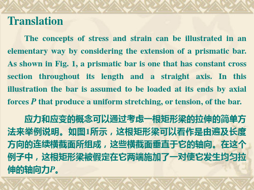
When a material exhibits a linear relationship between stress and strain, it is said to be linear elastic. This is an extremely important property of many solid materials, including most metals, plastics, wood, concrete, and ceramics. The linear relationship between stress and strain for a bar in tension can be expressed by the simple equation ζ=Eε (3) in which E is a constant of proportionality known as the modulus of elasticity for the material. 当一种材料的应力与应变表现出线性关系时，我们称这种材料为线弹性材料。这是许多固体材料的一个极其重要的性质，这些材料包括大多数金属，塑料，木材，混凝土和陶瓷。对于被拉伸的梁来说，这种应力与应变之间的线性关系可以用简单方程(3) ζ= Eε 来表示，这里E是一个已知的比例常数，即该材料的弹性模量。
方程(1) 用于求解在梁中均匀分布的应力问题。它表示了应力的单位是力除以面积。正如我们在图1中所看到的，当梁被力P拉伸的时候，生成的应力是拉应力；如果力的方向被颠倒，导致梁被压缩时，产生的应力被称为压应力。
A necessary condition for Eq.(1) to be valid is that the stress ζ must be uniform over the cross section of the bar. This condition will be realized if the axial force P acts through the centroid of the cross section. When the load P does not act at the centroid, bending of the bar will result, and a more complicated analysis is necessary. At present, however, it is assumed that all axial forces are applied at the centroid of the cross section unless specifically stated to the contrary. Also, unless stated otherwise, it is generally assumed that the weight of the object itself is neglected, as was done when discussing the bar in Fig.1.

弯曲正应力公式

σ = My Iz
(12.4)
物理条件：材料是线弹性材料所以可以应用胡克定律，即σ = Eε。线性变化的应变必然引起线性变化的应力。因此，如正应变的变化规律一样，正应力从在中性轴处的零应力线性地变化到离中性轴最远处的最大值。
静力学条件：由横截面上正应力的合力应为零可以确定中性轴的位置。
ε = a′b′ − ab = (ρ + y)dθ − ρdθ = y
ab
ρdθ
ρ
(12.1)
注意到中性层上的任意线不改变长度。根据定义，沿 a′b′的正应变可表示为：
47
Stresses in Beams
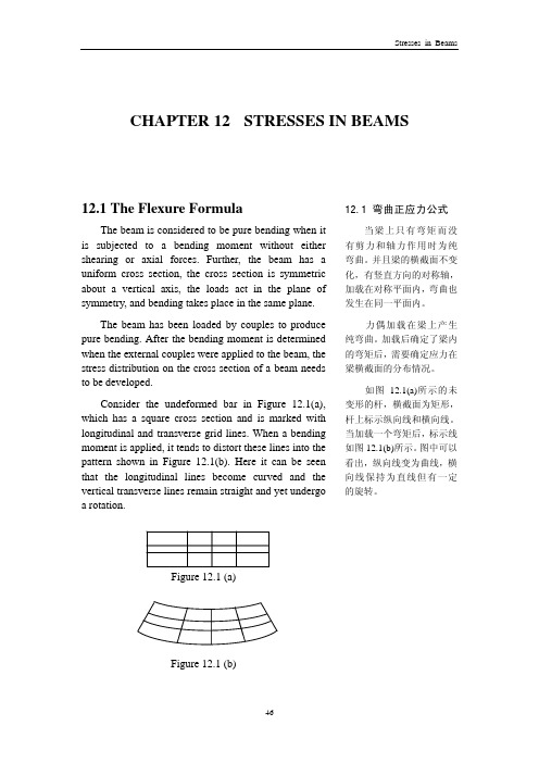
Physical Condition. The material behaves in a linear-elastic manner so that Hooke’s law applies, that is, σ = Eε. A linear variation of normal strain must then be the consequence of a linear variation in normal stress. Hence, like the normal strain variation, normal stress will vary from zero at the member’s neutral axis to a maximum value, a distance farthest from the neutral axis.
Equation 12.4 is often referred to as the flexure formula. It is used to determine the normal stress in a straight member, having a cross section that is symmetrical with respect to an axis, and the moment is applied perpendicular to this axis.

AASHTO 美国国家公路与运输协会标准

AASHTO 美国国家公路与运输协会标准AASHTO PMG-1-2001 路面管理指南Pavement Management GuideAASHTO GMPC-2-2002 指导方法和程序，在合同维修Guide for Methods and Procedures in Contract MaintenanceAASHTO GHOV-3-2004 指南高承载车辆（HOV ）设施Guide for High-Occupancy Vehicle (HOV) FacilitiesAASHTO GDPS-4-1993 指南设计路面结构Guide for Design of Pavement Structures AASHTO GDPS-3 V2-1986 指南设计路面结构第2卷-补充-1 998年Guide for Design of Pavement Structures Volume 2-Supplement - 1998AASHTO GDHS-5-2004 政策的几何设计的公路和街道-第五版Policy on Geometric Design of Highways and Streets-Fifth EditionAASHTO GDC-1-2003 准则设计constructibility -a ashto/ n sba钢桥协作-克 1 2.1-2003 Guidelines for Design for Constructibility - AASHTO/NSBA Steel Bridge Collaboration-G 12.1-2003 AASHTO GD-2-1965 政策上的几何设计的农村公路-撤回所取代aashto老人科日间医院A Policy on Geometric Design of Rural Highways-Withdrawn Replaced by AASHTO GDHS AASHTO GCPE-1996 指南订约，选拔，管理顾问公司在前期工程Guide for Contracting, Selecting, and Managing Consultants in Preconstruction EngineeringAASHTO FRBL-1-2002 交通运输投资在美国-货运铁路的底线报告Transportation Invest in America - Freight-Rail Bottom Line ReportAASHTO FHD-1-2004 指南实现的灵活性，在公路设计 A Guide to Achieving Flexibility in Highway DesignAASHTO FCAH-3-1990 信息指南剑击控制进入高速公路Informational Guide on Fencing Controlled Access HighwaysAASHTO ESC-2004 aashto中心环境方面的杰出表现-最佳做法，在竞争的环境管理AASHTO Center for Environmental Excellence - Best Practices in Environmental Stewardship Competition AASHTO EMCP-1992 评价和维修混凝土路面Evaluation and Maintenance of Concrete PavementsAASHTO DS-2005 一项政策的设计标准号州际公路系统5版A POLICY ON DESIGN STANDARDS INTERSTATE SYSTEM-Edition 5AASHTO DIVISION II 11.7-N/A 计量与支付Measurement and PaymentAASHTO DIVISION I 5.14-1996 重力及半重力墙的设计，和悬臂墙设计-中期1997年Gravity and Semi-Gravity Wall Design, and Cantilever Wall Design-Interim 1997AASHTO DIVISION I 5.13-1996 极限状态，负载因素和阻力因素，1997年中期Limit States, Load Factors and Resistance Factors-Interim 1997AASHTO DDPG-1-2003 设计图纸介绍指引Design Drawing Presentation GuidelinesAASHTO CSS-1-2005 中心环境方面的杰出表现最佳做法，在上下文敏感的解决方案Center for Environmental Excellence Best Practices in Context-Sensitive SolutionsAASHTO CSD-1-1998 不断变化的状态点The Changing State DOTAASHTO COMMENTARIES-2002 评标准规格为公路桥梁2002年第十七版Commentaries to Standard Specifications for Highway Bridges 2002-17th EditionAASHTO CM-4-1990 施工手册公路建设-第四版Construction Manual for HighwayConstruction-Fourth EditionAASHTO CA-3-2006 通勤在美国三-第三次国家报告对通勤的格局和趋势Commuting In America III - The Third National Report On Commuting Patterns and TrendsAASHTO BPCSS-2006 aashto中心环境方面的杰出表现-最佳做法，在上下文敏感的解决方案AASHTO Center for Environmental Excellence - Best Practices in Context-Sensitive Solutions AASHTO AU-5-2005 一政策对住宿的水电费与高速公路右侧的双向 A Policy On the Accommodation of Utilities Within Freeway Right-Of-WayAASHTO APPENDICES-2002 附录标准规格为公路桥梁2002年第十七版Appendices to Standard Specifications for Highway Bridges 2002-17th EditionAASHTO APH-1-2005 合作伙伴手册Partnering HandbookAASHTO APD-1-2005 加快项目交付。

Chapter_3_new

10
3.2.2 Solution (Continued)
a a ⇒ P e + Fa ⋅ − Fs ⋅ = 0 4 4 a ⇒ P e = ( Fs − Fa ) ⋅ 4 a = (σ s − σ a ) ⋅ ⋅ A 4 a 3 P 1 P a 1 = − = P⋅ ⋅ ⋅ 8 2 at 2 at 4 2at a ⇒e= 8
15
3.2.2 Solution to Ex. 3.2-3 (IV)
Solve LB'C 2 + LCD 2 +LB'D 2 ⇒ α ′ = sin −1 2LCD LB'C
−1
= 29.915 °
LB'C β ′ = cos cos α ′ = 44.912 ° LB'D
⇒ u total Px =± L AE
υ total
Px = mv h AE
wtotal
Px = mv b AE
8
3.2.2 Example 3.2-1
One half be aluminum the other half steel. Assume uniform elongation. ES / EA = 3. Determine stress distribution.
4
3.2 Axial Loading
3.2.1 Axial Stress
P σx = ± A
(3.2-1)
5
3.2.1 Axial Stress
Further limitations:
1. The load Px must go through the geometric centroid of the cross section A. For a given magnitude of force, the bending stress and deflections are greater when in compression versus tension. 2. For compressive loading, a stability problem called buckling can occur. If the magnitude of the force reaches the critical buckling load, the rod will begin to buckle or bend Eq(3.2-1) is no longer valid.

1、下载文档前请自行甄别文档内容的完整性，平台不提供额外的编辑、内容补充、找答案等附加服务。
2、"仅部分预览"的文档,不可在线预览部分如存在完整性等问题,可反馈申请退款(可完整预览的文档不适用该条件!)。
3、如文档侵犯您的权益，请联系客服反馈,我们会尽快为您处理(人工客服工作时间：9:00-18:30)。

115 - Uniform Sections subject to Bending 16. UNIFORM SECTIONS subject to BENDINGBending stressesWhen a uniform section of material is bent one side stretchesand the other compresses. At some point between the two thereis a plane where no stretching or compression occurs - this isknown as the neutral plane

Ry1

q󰀀

Neutralpla

top

bottom115 - Uniform Sections subject to Bending 2

original length = R xq󰀀Straintop =(R+y1) xq󰀀 - R xq󰀀R xq󰀀y

Length of bottom plane = (R-y2) xq󰀀original length = R xq󰀀

Strainbottom =(R-y2) xq󰀀 - R xq󰀀R xq󰀀y2Rs󰀀 = Ee󰀀buts󰀀 = yERs󰀀b = -EGenerally, if we measure y as positive above the neutral plane,and negative when below:s󰀀y=ER+-tensilestressescompressivestressesneutralplaney1Rs󰀀t = E&y2R= -

Length of top plane = (R+y1) xq󰀀115 - Uniform Sections subject to Bending 3s󰀀y

d󰀀y

Force = stress x area =s󰀀 xd󰀀y x wMoment = force x distanced󰀀M =s󰀀 xd󰀀y x w x yTo find the total moment we have to integrate from thetop to the bottom of the beam.

M =s󰀀 w y dyó󰀀õ󰀀

buts󰀀 = EyR

M = E y w y dyR

M = y² w dyER

This is a geometric property of the cross-sectionknown as the.It is an important section property given symbolI .

ó󰀀õ󰀀

The net effect of the internal stresses caused by the externallyapplied bending moment (M) must be equal and opposite to it.

Top half of the stressdistribution.w is thewidth of thebeam at distance yfrom the neutral plane

neutralplane115 - Uniform Sections subject to Bending 4

We can summarise the formulae for bending as below:

For any particular cross-section of beam we must either lookup theI-value in tables or calculate it from first principles.

This is known as the bending equation.M = external bending Moment applied (Nm).I = Second moment of area about the neutral plane. (m4)E = Elastic modulus of the material under bending.(N/m2)R = Radius of curvature of the beam at the where the bendingmoment (M) exists. (m)

= stress level in the beam (N/m2) at distancey (m) measuredfrom the neutral plane, above (+) or below (-) it.

Care - when using the Bending Equation make sure youusestandard SI unitsM often given in kNm [=103Nm]I often given in cm4 [= (10-2m)4 = 10-8m4]E often given in GN/m2 [ = 109 N/m2]s󰀀 often given in MN/m2 [ =106 N/m2]y may be in mm or cm [10-3 or 10-2 m]

M Es󰀀I R y= =115 - Uniform Sections subject to Bending 5Location of the Neutral Axis

?We divide the section intoshapes where weknow thecentroid position and find thetotal effect.

y2yA1

A1y1+A2y2=(A1+AFor 3 or more shapes it is

better to draw up a table.

Shape Area y Areax y123

-A1y1+A2y2

(A1+A2)y =

A(Ax y

y =-(Ax yA

The neutral axis of a beam’s cross-section always passesthrough the centroid of the section. i.e. the point (or line) aboutwhich the shape would balance.For symmetrical sections the centroid is at the centre.For unsymmetrical sections it has to be found bydividing into regular shapes, experimentally, or byusing a computer (CAD).

BENDING Section properties:115 - Uniform Sections subject to Bending 6

Second Moment of AreaFor certain geometrical shapes we can look up aformula which gives us theI-value about its neutral axis,otherwise it has to be found by dividing the shape intorecognised smaller shapes, or by using a computer(CAD).

When we have a composite section (one made up ofdifferent regular shapes) we cannot just add theI-values to obtain the totalI-value.We need to use theParallel Axis Theorem

IXX =Ina +Ay²IXX =I-value of the Area about axisX-XIna =I-value of the Area about itsown neutral axis n-ay = distance between the two axesX-X and n-aA = Area of the shape115 - Uniform Sections subject to Bending 7

Example - Find the position of the Neutral axis and theI-value of the section below: (lengths are in cm)

37-y

(for the section as a whole)

ShapeAyAyAy2Inaformula (cm2)(cm)(cm3)(cm4 )(cm4 )A16.007.00112.00784.005.33bd3/12B18.003.0054.00162.0054.00bd3/13Sum(S󰀀)34.00166.00946.0059.33

y =SA󰀀y/S󰀀AIXX =SA󰀀y2+S󰀀Ina=166/34=946 + 59.33=4.88cm=1005.33cm4

For the section as a wholeINA =IXX-Ay²=1005.33 - 34x4.882

=194.86cm4