Nonlinear Sigma Model Analysis of the AFM Phase Transition of the Kondo Lattice
matlab工具箱安装教程

1.1 如果是Matlab安装光盘上的工具箱,重新执行安装程序,选中即可;1.2 如果是单独下载的工具箱,一般情况下仅需要把新的工具箱解压到某个目录。
2 在matlab的file下面的set path把它加上。
3 把路径加进去后在file→Preferences→General的Toolbox Path Caching里点击update Toolbox Path Cache更新一下。
4 用which newtoolbox_command.m来检验是否可以访问。
如果能够显示新设置的路径,则表明该工具箱可以使用了。
把你的工具箱文件夹放到安装目录中“toolbox”文件夹中,然后单击“file”菜单中的“setpath”命令,打开“setpath”对话框,单击左边的“ADDFolder”命令,然后选择你的那个文件夹,最后单击“SAVE”命令就OK了。
MATLAB Toolboxes============================================/zsmcode.htmlBinaural-modeling software for MATLAB/Windows/home/Michael_Akeroyd/download2.htmlStatistical Parametric Mapping (SPM)/spm/ext/BOOTSTRAP MATLAB TOOLBOX.au/downloads/bootstrap_toolbox.htmlThe DSS package for MATLABDSS Matlab package contains algorithms for performing linear, deflation and symmetric DSS. http://www.cis.hut.fi/projects/dss/package/Psychtoolbox/download.htmlMultisurface Method Tree with MATLAB/~olvi/uwmp/msmt.htmlA Matlab Toolbox for every single topic !/~baum/toolboxes.htmleg. BrainStorm - MEG and EEG data visualization and processingCLAWPACK is a software package designed to compute numerical solutions to hyperbolic partial differential equations using a wave propagation approach/~claw/DIPimage - Image Processing ToolboxPRTools - Pattern Recognition Toolbox (+ Neural Networks)NetLab - Neural Network ToolboxFSTB - Fuzzy Systems ToolboxFusetool - Image Fusion Toolboxhttp://www.metapix.de/toolbox.htmWAVEKIT - Wavelet ToolboxGat - Genetic Algorithm ToolboxTSTOOL is a MATLAB software package for nonlinear time series analysis.TSTOOL can be used for computing: Time-delay reconstruction, Lyapunov exponents, Fractal dimensions, Mutual information, Surrogate data tests, Nearest neighbor statistics, Return times, Poincare sections, Nonlinear predictionhttp://www.physik3.gwdg.de/tstool/MATLAB / Data description toolboxA Matlab toolbox for data description, outlier and novelty detectionMarch 26, 2004 - D.M.J. Taxhttp://www-ict.ewi.tudelft.nl/~davidt/dd_tools/dd_manual.htmlMBEhttp://www.pmarneffei.hku.hk/mbetoolbox/Betabolic network toolbox for Matlabhttp://www.molgen.mpg.de/~lieberme/pages/network_matlab.htmlPharmacokinetics toolbox for Matlabhttp://page.inf.fu-berlin.de/~lieber/seiten/pbpk_toolbox.htmlThe SpiderThe spider is intended to be a complete object orientated environment for machine learning in Matlab. Aside from easy use of base learning algorithms, algorithms can be plugged together and can be compared with, e.g model selection, statistical tests and visual plots. This gives all the power of objects (reusability, plug together, share code) but also all the power of Matlab for machine learning research.http://www.kyb.tuebingen.mpg.de/bs/people/spider/index.htmlSchwarz-Christoffel Toolbox/matlabcentral/fileexchange/loadFile.do?objectId=1316&objectT ype=file#XML Toolbox/matlabcentral/fileexchange/loadFile.do?objectId=4278&object Type=fileFIR/TDNN Toolbox for MATLABBeta version of a toolbox for FIR (Finite Impulse Response) and TD (Time Delay) NeuralNetworks./interval-comp/dagstuhl.03/oish.pdfMisc.http://www.dcsc.tudelft.nl/Research/Software/index.htmlAstronomySaturn and Titan trajectories ... MALTAB astronomy/~abrecht/Matlab-codes/AudioMA Toolbox for Matlab Implementing Similarity Measures for Audiohttp://www.oefai.at/~elias/ma/index.htmlMAD - Matlab Auditory Demonstrations/~martin/MAD/docs/mad.htmMusic Analysis - Toolbox for Matlab : Feature Extraction from Raw Audio Signals for Content-Based Music Retrihttp://www.ai.univie.ac.at/~elias/ma/WarpTB - Matlab Toolbox for Warped DSPBy Aki Härmä and Matti Karjalainenhttp://www.acoustics.hut.fi/software/warp/MATLAB-related Softwarehttp://www.dpmi.tu-graz.ac.at/~schloegl/matlab/Biomedical Signal data formats (EEG machine specific file formats with Matlab import routines)http://www.dpmi.tu-graz.ac.at/~schloegl/matlab/eeg/MPEG Encoding library for MATLAB Movies (Created by David Foti)It enables MATLAB users to read (MPGREAD) or write (MPGWRITE) MPEG movies. That should help Video Quality project.Filter Design packagehttp://www.ee.ryerson.ca:8080/~mzeytin/dfp/index.htmlOctave by Christophe COUVREUR (Generates normalized A-weigthing, C-weighting, octave and one-third-octave digital filters)/matlabcentral/fileexchange/loadFile.do?objectType=file&object Id=69Source Coding MATLAB Toolbox/users/kieffer/programs.htmlBio Medical Informatics (Top)CGH-Plotter: MATLAB Toolbox for CGH-data AnalysisCode: http://sigwww.cs.tut.fi/TICSP/CGH-Plotter/Poster: http://sigwww.cs.tut.fi/TICSP/CSB2003/Posteri_CGH_Plotter.pdfThe Brain Imaging Software Toolboxhttp://www.bic.mni.mcgill.ca/software/MRI Brain Segmentation/matlabcentral/fileexchange/loadFile.do?objectId=4879Chemometrics (providing PCA) (Top)Matlab Molecular Biology & Evolution Toolbox(Toolbox Enables Evolutionary Biologists to Analyze and View DNA and Protein Sequences) James J. Caihttp://www.pmarneffei.hku.hk/mbetoolbox/Toolbox provided by Prof. Massart research grouphttp://minf.vub.ac.be/~fabi/publiek/Useful collection of routines from Prof age smilde research grouphttp://www-its.chem.uva.nl/research/pacMultivariate Toolbox written by Rune Mathisen/~mvartools/index.htmlMatlab code and datasetshttp://www.acc.umu.se/~tnkjtg/chemometrics/dataset.htmlChaos (Top)Chaotic Systems Toolbox/matlabcentral/fileexchange/loadFile.do?objectId=1597&objectT ype=file#HOSA Toolboxhttp://www.mathworks.nl/matlabcentral/fileexchange/loadFile.do?objectId=3013&objectTy pe=fileChemistry (Top)MetMAP - (Metabolical Modeling, Analysis and oPtimization alias Met. M. A. P.)http://webpages.ull.es/users/sympbst/pag_ing/pag_metmap/index.htmDoseLab - A set of software programs for quantitative comparison of measured and computed radiation dose distributions/GenBank Overview/Genbank/GenbankOverview.htmlMatlab: /matlabcentral/fileexchange/loadFile.do?objectId=1139CodingCode for the estimation of Scaling Exponentshttp://www.cubinlab.ee.mu.oz.au/~darryl/secondorder_code.htmlControl (Top)Control Tutorial for Matlab/group/ctm/AnotherCommunications (Top)Channel Learning Architecture toolbox(This Matlab toolbox is a supplement to the article "HiperLearn: A High Performance Learning Architecture")http://www.isy.liu.se/cvl/Projects/hiperlearn/Source Coding MATLAB Toolbox/users/kieffer/programs.htmlTCP/UDP/IP Toolbox 2.0.4/matlabcentral/fileexchange/loadFile.do?objectId=345&objectT ype=fileHome Networking Basis: Transmission Environments and Wired/Wireless Protocols Walter Y. Chen/support/books/book5295.jsp?category=new&language=-1MATLAB M-files and Simulink models/matlabcentral/fileexchange/loadFile.do?objectId=3834&object Type=file•OPNML/MATLAB Facilities/OPNML_Matlab/Mesh Generation/home/vavasis/qmg-home.htmlOpenFEM : An Open-Source Finite Element Toolbox/CALFEM is an interactive computer program for teaching the finite element method (FEM)http://www.byggmek.lth.se/Calfem/frinfo.htmThe Engineering Vibration Toolbox/people/faculty/jslater/vtoolbox/vtoolbox.htmlSaGA - Spatial and Geometric Analysis Toolboxby Kirill K. Pankratov/~glenn/kirill/saga.htmlMexCDF and NetCDF Toolbox For Matlab-5&6/staffpages/cdenham/public_html/MexCDF/nc4ml5.htmlCUEDSID: Cambridge University System Identification Toolbox/jmm/cuedsid/Kriging Toolbox/software/Geostats_software/MATLAB_KRIGING_TOOLBOX.htmMonte Carlo (Dr Nando)http://www.cs.ubc.ca/~nando/software.htmlRIOTS - The Most Powerful Optimal Control Problem Solver/~adam/RIOTS/ExcelMATLAB xlsheets/matlabcentral/fileexchange/loadFile.do?objectId=4474&objectTy pe=filewrite2excel/matlabcentral/fileexchange/loadFile.do?objectId=4414&objectTy pe=fileFinite Element Modeling (FEM) (Top)OpenFEM - An Open-Source Finite Element Toolbox/NLFET - nonlinear finite element toolbox for MATLAB ( framework for setting up, solving, and interpreting results for nonlinear static and dynamic finite element analysis.)/GetFEM - C++ library for finite element methods elementary computations with a Matlabinterfacehttp://www.gmm.insa-tlse.fr/getfem/FELIPE - FEA package to view results ( contains neat interface to MATLA/~blstmbr/felipe/Finance (Top)A NEW MATLAB-BASED TOOLBOX FOR COMPUTER AIDED DYNAMIC TECHNICAL TRADINGStephanos Papadamou and George StephanidesDepartment of Applied Informatics, University Of Macedonia Economic & Social Sciences, Thessaloniki, Greece/fen31/one_time_articles/dynamic_tech_trade_matlab6.htm Paper: :8089/eps/prog/papers/0201/0201001.pdfCompEcon Toolbox for Matlab/~pfackler/compecon/toolbox.htmlGenetic Algorithms (Top)The Genetic Algorithm Optimization Toolbox (GAOT) for Matlab 5/mirage/GAToolBox/gaot/Genetic Algorithm ToolboxWritten & distributed by Andy Chipperfield (Sheffield University, UK)/uni/projects/gaipp/gatbx.htmlManual: /~gaipp/ga-toolbox/manual.pdfGenetic and Evolutionary Algorithm Toolbox (GEATbx)/Evolutionary Algorithms for MATLAB/links/ea_matlab.htmlGenetic/Evolutionary Algorithms for MATLABhttp://www.systemtechnik.tu-ilmenau.de/~pohlheim/EA_Matlab/ea_matlab.html GraphicsVideoToolbox (C routines for visual psychophysics on Macs by Denis Pelli)/VideoToolbox/Paper: /pelli/pubs/pelli1997videotoolbox.pdf4D toolbox/~daniel/links/matlab/4DToolbox.htmlImages (Top)Eyelink Toolbox/eyelinktoolbox/Paper: /eyelinktoolbox/EyelinkToolbox.pdfCellStats: Automated statistical analysis of color-stained cell images in Matlabhttp://sigwww.cs.tut.fi/TICSP/CellStats/SDC Morphology Toolbox for MATLAB (powerful collection of latest state-of-the-art gray-scale morphological tools that can be applied to image segmentation, non-linear filtering, pattern recognition and image analysis)/Image Acquisition Toolbox/products/imaq/Halftoning Toolbox for MATLAB/~bevans/projects/halftoning/toolbox/index.htmlDIPimage - A Scientific Image Processing Toolbox for MATLABhttp://www.ph.tn.tudelft.nl/DIPlib/dipimage_1.htmlPNM Toolboxhttp://home.online.no/~pjacklam/matlab/software/pnm/index.htmlAnotherICA / KICA and KPCA (Top)ICA TU Toolboxhttp://mole.imm.dtu.dk/toolbox/menu.htmlMISEP Linear and Nonlinear ICA Toolboxhttp://neural.inesc-id.pt/~lba/ica/mitoolbox.htmlKernel Independant Component Analysis/~fbach/kernel-ica/index.htmMatlab: kernel-ica version 1.2KPCA- Please check the software section of kernel machines.KernelStatistical Pattern Recognition Toolboxhttp://cmp.felk.cvut.cz/~xfrancv/stprtool/MATLABArsenal A MATLAB Wrapper for Classification/tmp/MATLABArsenal.htmMarkov (Top)MapHMMBOX 1.1 - Matlab toolbox for Hidden Markov Modelling using Max. Aposteriori EM Prerequisites: Matlab 5.0, Netlab. Last Updated: 18 March 2002./~parg/software/maphmmbox_1_1.tarHMMBOX 4.1 - Matlab toolbox for Hidden Markov Modelling using Variational Bayes Prerequisites: Matlab 5.0,Netlab. Last Updated: 15 February 2002../~parg/software/hmmbox_3_2.tar/~parg/software/hmmbox_4_1.tarMarkov Decision Process (MDP) Toolbox for MatlabKevin Murphy, 1999/~murphyk/Software/MDP/MDP.zipMarkov Decision Process (MDP) Toolbox v1.0 for MATLABhttp://www.inra.fr/bia/T/MDPtoolbox/Hidden Markov Model (HMM) Toolbox for Matlab/~murphyk/Software/HMM/hmm.htmlBayes Net Toolbox for Matlab/~murphyk/Software/BNT/bnt.htmlMedical (Top)EEGLAB Open Source Matlab Toolbox for Physiological Research (formerly ICA/EEG Matlabtoolbox)/~scott/ica.htmlMATLAB Biomedical Signal Processing Toolbox/Toolbox/Powerful package for neurophysiological data analysis ( Igor Kagan webpage)/Matlab/Unitret.htmlEEG / MRI Matlab Toolbox/Microarray data analysis toolbox (MDAT): for normalization, adjustment and analysis of gene expression_r data.Knowlton N, Dozmorov IM, Centola M. Department of Arthritis and Immunology, Oklahoma Medical Research Foundation, Oklahoma City, OK, USA 73104. We introduce a novel Matlab toolbox for microarray data analysis. This toolbox uses normalization based upon a normally distributed background and differential gene expression_r based on 5 statistical measures. The objects in this toolbox are open source and can be implemented to suit your application. AVAILABILITY: MDAT v1.0 is a Matlab toolbox and requires Matlab to run. MDAT is freely available at:/publications/2004/knowlton/MDAT.zipMIDI (Top)MIDI Toolbox version 1.0 (GNU General Public License)http://www.jyu.fi/musica/miditoolbox/Misc. (Top)MATLAB-The Graphing Tool/~abrecht/matlab.html3-D Circuits The Circuit Animation Toolbox for MATLAB/other/3Dcircuits/SendMailhttp://carol.wins.uva.nl/~portegie/matlab/sendmail/Coolplothttp://www.reimeika.ca/marco/matlab/coolplots.htmlMPI (Matlab Parallel Interface)Cornell Multitask Toolbox for MATLAB/Services/Software/CMTM/Beolab Toolbox for v6.5Thomas Abrahamsson (Professor, Chalmers University of Technology, Applied Mechanics,Göteborg, Sweden)http://www.mathworks.nl/matlabcentral/fileexchange/loadFile.do?objectId=1216&objectType =filePARMATLABNeural Networks (Top)SOM Toolboxhttp://www.cis.hut.fi/projects/somtoolbox/Bayes Net Toolbox for Matlab/~murphyk/Software/BNT/bnt.htmlNetLab/netlab/Random Neural Networks/~ahossam/rnnsimv2/ftp: ftp:///pub/contrib/v5/nnet/rnnsimv2/NNSYSID Toolbox (tools for neural network based identification of nonlinear dynamic systems) http://www.iau.dtu.dk/research/control/nnsysid.htmlOceanography (Top)WAFO. Wave Analysis for Fatigue and Oceanographyhttp://www.maths.lth.se/matstat/wafo/ADCP toolbox for MATLAB (USGS, USA)Presented at the Hydroacoustics Workshop in Tampa and at ADCP's in Action in San Diego /operations/stg/pubs/ADCPtoolsSEA-MAT - Matlab Tools for Oceanographic AnalysisA collaborative effort to organize and distribute Matlab tools for the Oceanographic Community /Ocean Toolboxhttp://www.mar.dfo-mpo.gc.ca/science/ocean/epsonde/programming.htmlEUGENE D. GALLAGHER(Associate Professor, Environmental, Coastal & Ocean Sciences)/edgwebp.htmOptimization (Top)MODCONS - a MATLAB Toolbox for Multi-Objective Control System Design/mecheng/jfw/modcons.htmlLazy Learning Packagehttp://iridia.ulb.ac.be/~lazy/SDPT3 version 3.02 -- a MATLAB software for semidefinite-quadratic-linear programming .sg/~mattohkc/sdpt3.htmlMinimum Enclosing Balls: Matlab Code/meb/SOSTOOLS Sum of Squares Optimi zation Toolbox for MATLAB User’s guide/sostools/sostools.pdfPSOt - a Particle Swarm Optimization Toolbox for use with MatlabBy Brian Birge ... A Particle Swarm Optimization Toolbox (PSOt) for use with the Matlab scientific programming environment has been developed. PSO isintroduced briefly and then the use of the toolbox is explained with some examples. A link to downloadable code is provided.Plot/software/plotting/gbplot/Signal Processing (Top)Filter Design with Motorola DSP56Khttp://www.ee.ryerson.ca:8080/~mzeytin/dfp/index.htmlChange Detection and Adaptive Filtering Toolboxhttp://www.sigmoid.se/Signal Processing Toolbox/products/signal/ICA TU Toolboxhttp://mole.imm.dtu.dk/toolbox/menu.htmlTime-Frequency Toolbox for Matlabhttp://crttsn.univ-nantes.fr/~auger/tftb.htmlVoiceBox - Speech Processing Toolbox/hp/staff/dmb/voicebox/voicebox.htmlLeast Squared - Support Vector Machines (LS-SVM)http://www.esat.kuleuven.ac.be/sista/lssvmlab/WaveLab802 : the Wavelet ToolboxBy David Donoho, Mark Reynold Duncan, Xiaoming Huo, Ofer Levi /~wavelab/Time-series Matlab scriptshttp://wise-obs.tau.ac.il/~eran/MATLAB/TimeseriesCon.htmlUvi_Wave Wavelet Toolbox Home Pagehttp://www.gts.tsc.uvigo.es/~wavelets/index.htmlAnotherSupport Vector Machine (Top)MATLAB Support Vector Machine ToolboxDr Gavin CawleySchool of Information Systems, University of East Anglia/~gcc/svm/toolbox/LS-SVM - SISTASVM toolboxes/dmi/svm/LSVM Lagrangian Support Vector Machine/dmi/lsvm/Statistics (Top)Logistic regression/SAGA/software/saga/Multi-Parametric Toolbox (MPT) A tool (not only) for multi-parametric optimization. http://control.ee.ethz.ch/~mpt/ARfit: A Matlab package for the estimation of parameters and eigenmodes of multivariate autoregressive modelshttp://www.mat.univie.ac.at/~neum/software/arfit/The Dimensional Analysis Toolbox for MATLABHome: http://www.sbrs.de/Paper: http://www.isd.uni-stuttgart.de/~brueckner/Papers/similarity2002.pdfFATHOM for Matlab/personal/djones/PLS-toolbox/Multivariate analysis toolbox (N-way Toolbox - paper)http://www.models.kvl.dk/source/nwaytoolbox/index.aspClassification Toolbox for Matlabhttp://tiger.technion.ac.il/~eladyt/classification/index.htmMatlab toolbox for Robust Calibrationhttp://www.wis.kuleuven.ac.be/stat/robust/toolbox.htmlStatistical Parametric Mapping/spm/spm2.htmlEVIM: A Software Package for Extreme Value Analysis in Matlabby Ramazan Gençay, Faruk Selcuk and Abdurrahman Ulugulyagci, 2001.Manual (pdf file) evim.pdf - Software (zip file) evim.zipTime Series Analysishttp://www.dpmi.tu-graz.ac.at/~schloegl/matlab/tsa/Bayes Net Toolbox for MatlabWritten by Kevin Murphy/~murphyk/Software/BNT/bnt.htmlOther: /information/toolboxes.htmlARfit: A Matlab package for the estimation of parameters and eigenmodes of multivariate autoregressive models/~tapio/arfit/M-Fithttp://www.ill.fr/tas/matlab/doc/mfit4/mfit.htmlDimensional Analysis Toolbox for Matlab/The NaN-toolbox: A statistic-toolbox for Octave and Matlab®... handles data with and without MISSING VALUES.http://www-dpmi.tu-graz.ac.at/~schloegl/matlab/NaN/Iterative Methods for Optimization: Matlab Codes/~ctk/matlab_darts.htmlMultiscale Shape Analysis (MSA) Matlab Toolbox 2000p.br/~cesar/projects/multiscale/Multivariate Ecological & Oceanographic Data Analysis (FATHOM)From David Jones/personal/djones/glmlab (Generalized Linear Models in MATLA.au/staff/dunn/glmlab/glmlab.htmlSpacial and Geometric Analysis (SaGA) toolboxInteresting audio links with FAQ, VC++, on the topic机器学习网站北京大学视觉与听觉信息处理实验室北京邮电大学模式识别与智能系统学科复旦大学智能信息处理开放实验室IEEE Computer Society北京映象站点计算机科学论坛机器人足球赛模式识别国家重点实验室南京航空航天大学模式识别与神经计算实验室- PARNEC南京大学机器学习与数据挖掘研究所- LAMDA南京大学人工智能实验室南京大学软件新技术国家重点实验室人工生命之园数据挖掘研究院微软亚洲研究院中国科技大学人工智能中心中科院计算所中科院计算所生物信息学实验室中科院软件所中科院自动化所中科院自动化所人工智能实验室ACL Special Interest Group on Natural Language Learning (SIGNLL)ACMACM Digital LibraryACM SIGARTACM SIGIRACM SIGKDDACM SIGMODAdaptive Computation Group at University of New MexicoAI at Johns HopkinsAI BibliographiesAI Topics: A dynamic online library of introductory information about artificial intelligence Ant Colony OptimizationARIES Laboratory: Advanced Research in Intelligent Educational SystemsArtificial Intelligence Research in Environmental Sciences (AIRIES)Austrian Research Institute for AI (OFAI)Back Issues of Neuron DigestBibFinder: a computer science bibliography search engine integrating many other engines BioAPI ConsortiumBiological and Computational Learning Center at MITBiometrics ConsortiumBoosting siteBrain-Style Information Systems Research Group at RIKEN Brain Science Institute, Japan British Computer Society Specialist Group on Expert SystemsCanadian Society for Computational Studies of Intelligence (CSCSI)CI Collection of BibTex DatabasesCITE, the first-stop source for computational intelligence information and services on the web Classification Society of North AmericaCMU Advanced Multimedia Processing GroupCMU Web->KB ProjectCognitive and Neural Systems Department of Boston UniversityCognitive Sciences Eprint Archive (CogPrints)COLT: Computational Learning TheoryComputational Neural Engineering Laboratory at the University of FloridaComputational Neurobiology Lab at California, USAComputer Science Department of National University of SingaporeData Mining Server Online held by Rudjer Boskovic InstituteDatabase Group at Simon Frazer University, CanadaDBLP: Computer Science BibliographyDigital Biology: about creating artificial lifeDistributed AI Unit at Queen Mary & Westfield College, University of LondonDistributed Artificial Intelligence at HUJIDSI Neural Networks group at the Université di Firenze, ItalyEA-related literature at the EvALife research group at DAIMI, University of Aarhus, Denmark Electronic Research Group at Aberdeen UniversityElsevierComputerScienceEuropean Coordinating Committee for Artificial Intelligence (ECCAI)European Network of Excellence in ML (MLnet)European Neural Network Society (ENNS)Evolutionary Computing Group at University of the West of EnglandEvolutionary Multi-Objective Optimization RepositoryExplanation-Based Learning at University of Illinoise at Urbana-ChampaignFace Detection HomepageFace Recognition Vendor TestFace Recognition HomepageFace Recognition Research CommunityFingerpassftp of Jude Shavlik's Machine Learning Group (University of Wisconsin-Madison)GA-List Searchable DatabaseGenetic Algorithms Digest ArchiveGenetic Programming BibliographyGesture Recognition HomepageHCI Bibliography Project contain extended bibliographic information (abstract, key words, table of contents, section headings) for most publications Human-Computer Interaction dating back to 1980 and selected publications before 1980IBM ResearchIEEEIEEE Computer SocietyIEEE Neural Networks SocietyIllinois Genetic Algorithms Laboratory (IlliGAL)ILP Network of ExcellenceInductive Learning at University of Illinoise at Urbana-ChampaignIntelligent Agents RepositoryIntellimedia Project at North Carolina State UniversityInteractive Artificial Intelligence ResourcesInternational Association of Pattern RecognitionInternational Biometric Industry AssociationInternational Joint Conference on Artificial Intelligence (IJCAI)International Machine Learning Society (IMLS)International Neural Network Society (INNS)Internet Softbot Research at University of WashingtonJapanese Neural Network Society (JNNS)Java Agents for Meta-Learning Group (JAM) at Computer Science Department, Columbia University, for Fraud and Intrusion Detection Using Meta-Learning AgentsKernel MachinesKnowledge Discovery MineLaboratory for Natural and Simulated Cognition at McGill University, CanadaLearning Laboratory at Carnegie Mellon UniversityLearning Robots Laboratory at Carnegie Mellon UniversityLaboratoire d'Informatique et d'Intelligence Artificielle (IIA-ENSAIS)Machine Learning Group of Sydney University, AustraliaMammographic Image Analysis SocietyMDL Research on the WebMirek's Cellebration: 1D and 2D Cellular Automata explorerMIT Artificial Intelligence LaboratoryMIT Media LaboratoryMIT Media Laboratory Vision and Modeling GroupMLNET: a European network of excellence in Machine Learning, Case-based Reasoning and Knowledge AcquisitionMLnet Machine Learning Archive at GMD includes papers, software, and data sets MIRALab at University of Geneva: leading research on virtual human simulationNeural Adaptive Control Technology (NACT)Neural Computing Research Group at Aston University, UKNeural Information Processing Group at Technical University of BerlinNIPSNIPS OnlineNeural Network Benchmarks, Technical Reports,and Source Code maintained by Scott Fahlman at CMU; source code includes Quickprop, Cascade-Correlation, Aspirin/Migraines Neural Networks FAQ by Lutz PrecheltNeural Networks FAQ by Warren S. SarleNeural Networks: Freeware and Shareware ToolsNeural Network Group at Department of Medical Physics and Biophysics, University ofNeural Network Group at Université Catholique de LouvainNeural Network Group at Eindhoven University of TechnologyNeural Network Hyperplane Animator program that allows easy visualization of training data and weights in a back-propagation neural networkNeural Networks Research at TUT/ELENeural Networks Research Centre at Helsinki University of Technology, FinlandNeural Network Speech Group at Carnegie Mellon UniversityNeural Text Classification with Neural NetworksNonlinearity and Complexity HomepageOFAI and IMKAI library information system, provided by the Department of Medical Cybernetics and Artificial Intelligence at the University of Vienna (IMKAI) and the Austrian Research Institute for Artificial Intelligence (OFAI). It contains over 36,000 items (books, research papers, conference papers, journal articles) from many subareas of AI OntoWeb: Ontology-based information exchange for knowledge management and electronic commercePortal on Neural Network ForecastingPRAG: Pattern Recognition and Application Group at University of CagliariQuest Project at IBM Almaden Research Center: an academic website focusing on classification and regression trees. Maintained by Tjen-Sien LimReinforcement Learning at Carnegie Mellon UniversityResearchIndex: NECI Scientific Literature Digital Library, indexing over 200,000 computer science articlesReVision: Reviewing Vision in the Web!RIKEN: The Institute of Physical and Chemical Research, JapanSalford SystemsSANS Studies of Artificial Neural Systems, at the Royal Institute of Technology, Sweden Santa-Fe InstituteScirus: a search engine locating scientific information on the InternetSecond Moment: The News and Business Resource for Applied AnalyticsSEL-HPC Article Archive has sections for neural networks, distributed AI, theorem proving, and a variety of other computer science topicsSOAR Project at University of Southern CaliforniaSociety for AI and StatisticsSVM of ANU CanberraSVM of Bell LabsSVM of GMD-First BerlinSVM of MITSVM of Royal Holloway CollegeSVM of University of SouthamptonSVM-workshop at NIPS97TechOnLine: TechOnLine University offers free online courses and lecturesUCI Machine Learning GroupUMASS Distributed Artificial Intelligence LaboratoryUTCS Neural Networks Research Group of Artificial Intelligence Lab, Computer Science Department, University of Texas at AustinVivisimo Document Clustering: a powerful search engine which returns clustered results Worcester Polytechnic Institute Artificial Intelligence Research Group (AIRG)Xerion neural network simulator developed and used by the connectionist group at the University of TorontoYale's CTAN Advanced Technology Center for Theoretical and Applied Neuroscience ZooLand: Artificial Life Resource。
药剂学英文术语

生物药剂学英文汉译英要求Biopharmaceutics生物药剂学Absorption吸收Distribution分布Metabolism代谢Excretion排泄Transport转运Disposition处置Elimination消除Transcellular pathway细胞通道转运Paracellular pathway细胞旁路通道转运Passive transport被动转运Pore transport膜孔转运Carrier-mediated transport载体媒介转运Facilitated diffusion易化扩散、促进扩散Active transport主动转运Membrane mobile transport膜动转运Pinocytosis胞饮作用Phagocytosis吞噬作用First pass effect首过效应pH-partition hypothesis pH-分配假说Dissolution溶出Parenteral drug delivery注射给药Oral cavity mucosa drug delivery口腔粘膜给药Transdermal drug delivery皮肤给药Nasal mucosa drug delivery鼻粘膜给药Pulmonary drug delivery肺部给药Rectal drug delivery直肠给药Ophthalmic drug delivery眼部给药Distribution分布Accumulation蓄积Apparent volume of distribution表观分布容积Metabolize, metabolism代谢Biotransformation生物转化Inhibition酶抑制作用Inhibitor酶抑制剂Induction酶诱导作用Inducer酶诱导剂英译汉要求Membrane transport膜转运Fluid mosaic model生物膜液态镶嵌模型Extrinsic proteins外在蛋白Intrinsic proteins内在蛋白Fluidity流动性Asymmetry不对称性Semipermeability半透性P-glycoprotein P糖蛋白Vesicle小泡Endocytosis入胞作用Exocytosis出胞作用Kerckring环状褶壁Villi绒毛Epithelium cell上皮细胞Microvilli微绒毛Apical membrane顶侧膜Brush border membrane刷状缘膜Basal membrane基底膜Lateral membrane侧细胞膜Tight junction紧密结合Solvent drag effect溶媒牵引效应Gastric emptying rate胃空速率Liver first pass effect肝首过效应Lymphatic circulation淋巴循环Ionization解离度Lipophilicity脂溶性Dissolution rate溶出速率Molecular weight分子量Oil-water partition coefficient油水分配系数Sink condition漏槽条件Critical particle size, CPS临界粒径Polymorphism多晶型Absorption number, An吸收指数Dose number, Do剂量指数Dissolution number, Dn溶出指数Permeation enhancer透过促进剂或Absorption enhancer吸收促进剂Solid dispersion tech固体分散技术Dispersible tablet分散片Effervescent tablet泡腾片Sustained-release preparation缓释制剂Controlled-release preparation控释制剂Stability稳定性Day/night rhythm昼夜节律Site-specific drug delivery system定位释药系统Oral delayed-release preparation口服迟释制剂Stomach-specific preparation口服胃滞留制剂Floating漂浮型Swelling膨胀型Sticking粘附型Intestine-specific preparation小肠迟释制剂Oral colon-specific drug delivery system, OCDDS口服结肠定位给药系统In vitro experimental model离体实验模型Tissue flux chambers组织流动室法Mucosa粘膜Secosa浆膜Everted gut sac外翻肠囊法Everted rings外翻环法In situ experimental model原位实验模型Intestine perfusion method肠道灌流法In vivo experimental model体内法Intravenous injection静脉注射Intramuscular injection肌内注射Hypodermic injection皮下注射Intradermic injection皮内注射Solid particle precipitation固体粒子析出Masticatory mucosa咀嚼粘膜Lining mucosa内衬粘膜Specialized mucosa特性粘膜Buccal mucosa颊粘膜Sublingual mucosa舌下粘膜Transdermal drug delivery system, TDDS/Transdermal therapeutic system经皮给药系统Physiologic factors生理因素Iontophoresis离子导入技术Cilia movement纤毛运动Surfactant表面活性剂Eyelid眼睑Eye adjunct眼附属器Cornea角膜Drug-protein binding药物-蛋白结合Albumin白蛋白Alpha acid glycoprotein, AAG α1-酸性糖蛋白Lipoprotein脂蛋白Binding constant结合常数Blood-brain barrier血-脑脊液屏障Inter-membrane transfer膜间转运Contact release接触释放Adsorption吸附Fusion融合Endocytosis内吞Pinocytosis胞饮Long-circulating DDS长循环微粒给药系统Target drug delivery system靶向给药系统Intracellular target of biomacromolecule生物技术药物的细胞内靶向Liver microsome enzymes微粒体药物代谢酶系Live microsome mixed function monooxygenase肝微粒体混合功能氧化酶或单加氧酶Glucuronyl transferase葡萄糖醛酸转移酶The first phase reaction第一相反应Combination reaction结合反应Optical isomerism光学异构Cortex皮质Medulla髓质Nephron肾单位Glomerular filtration肾小球滤过Active tubular secretion肾小管分泌Tubular reabsorption肾小管重吸收Inulin菊粉Biliary excretion胆汁排泄Renal clearance肾清除率Enterohepatic cycle肠肝循环Compartment model隔室模型Single compartment mode一室模型Two compartment model二室模型Multicompartment model多室模型First order processes一级速度过程Zero order processes零级速度过程Nonlinear processes非线性速度过程Pharmacokinetics, PK药物动力学Population pharmacokinetics, PPK群体药物动力学Clinical pharmacokinetics临床药物动力学Therapeutic drug monitoring, TDM治疗药物监测Chronopharmacokinetics时辰药物动力学Physiological pharmacokinetic model生理药物动力学模型Biological half life生物半衰期Sigma-minus method亏量法,又称总和-减量法Steady-state drug concentration稳态血药浓度Loading dose负荷剂量Lag time滞后时间Extravascular delivery血管外给药Plateau level坪浓度Fluctuation percentage, FI波动百分数Degree of fluctuation, DF波动度Product inhibition产物抑制Plasma drug concentration change percentage血药浓度变化率Capacity-limited process容量限制过程Design of dosage regimen临床给药方案设计Individualization of drug dosage regimes给药方案个体化Bioavailability生物利用度Extent of bioavailability, EBA生物利用程度Rate of bioavailability, RBA生物利用速度Absolute bioavailability, Fabs绝对生物利用度Relative bioavailability, Frel相对生物利用度Pharmaceutical equivalence药剂等效性Bioequivalence生物等效性。
NONMEM软件使用说明书:非线性混合效应模型理解与应用
Package‘nmw’May10,2023Version0.1.5Title Understanding Nonlinear Mixed Effects Modeling for PopulationPharmacokineticsDescription This shows how NONMEM(R)software works.NONMEM's classical estimation meth-ods like'First Order(FO)approximation','First Order Conditional Estima-tion(FOCE)',and'Laplacian approximation'are explained.Depends R(>=3.5.0),numDerivByteCompile yesLicense GPL-3Copyright2017-,Kyun-Seop BaeAuthor Kyun-Seop BaeMaintainer Kyun-Seop Bae<********>URL https:///package=nmwNeedsCompilation noRepository CRANDate/Publication2023-05-1003:40:02UTCR topics documented:nmw-package (2)AddCox (3)CombDmExPc (4)CovStep (5)EstStep (6)InitStep (7)TabStep (9)TrimOut (10)Index1112nmw-package nmw-package Understanding Nonlinear Mixed Effects Modeling for PopulationPharmacokineticsDescriptionThis shows how NONMEM(R)</innovation/nonmem/>software works. DetailsThis package explains’First Order(FO)approximation’method,’First Order Conditional Estima-tion(FOCE)’method,and’Laplacian(LAPL)’method of NONMEM software.Author(s)Kyun-Seop Bae<********>References1.NONMEM Users guide2.Wang Y.Derivation of various NONMEM estimation methods.J Pharmacokinet Pharmaco-dyn.2007.3.Kang D,Bae K,Houk BE,Savic RM,Karlsson MO.Standard Error of Empirical BayesEstimate in NONMEM(R)VI.K J Physiol Pharmacol.2012.4.Kim M,Yim D,Bae K.R-based reproduction of the estimation process hidden behind NON-MEM Part1:First order approximation method.2015.5.Bae K,Yim D.R-based reproduction of the estimation process hidden behind NONMEM Part2:First order conditional estimation.2016.ExamplesDataAll=Theophcolnames(DataAll)=c("ID","BWT","DOSE","TIME","DV")DataAll[,"ID"]=as.numeric(as.character(DataAll[,"ID"]))nTheta=3nEta=3nEps=2THETAinit=c(2,50,0.1)OMinit=matrix(c(0.2,0.1,0.1,0.1,0.2,0.1,0.1,0.1,0.2),nrow=nEta,ncol=nEta) SGinit=diag(c(0.1,0.1))LB=rep(0,nTheta)#Lower boundUB=rep(1000000,nTheta)#Upper boundFGD=deriv(~DOSE/(TH2*exp(ETA2))*TH1*exp(ETA1)/(TH1*exp(ETA1)-TH3*exp(ETA3))*(exp(-TH3*exp(ETA3)*TIME)-exp(-TH1*exp(ETA1)*TIME)),AddCox3 c("ETA1","ETA2","ETA3"),function.arg=c("TH1","TH2","TH3","ETA1","ETA2","ETA3","DOSE","TIME"),func=TRUE,hessian=TRUE)H=deriv(~F+F*EPS1+EPS2,c("EPS1","EPS2"),function.arg=c("F","EPS1","EPS2"),func=TRUE) PRED=function(THETA,ETA,DATAi){FGDres=FGD(THETA[1],THETA[2],THETA[3],ETA[1],ETA[2],ETA[3],DOSE=320,DATAi[,"TIME"]) Gres=attr(FGDres,"gradient")Hres=attr(H(FGDres,0,0),"gradient")if(e$METHOD=="LAPL"){Dres=attr(FGDres,"hessian")Res=cbind(FGDres,Gres,Hres,Dres[,1,1],Dres[,2,1],Dres[,2,2],Dres[,3,])colnames(Res)=c("F","G1","G2","G3","H1","H2","D11","D21","D22","D31","D32","D33") }else{Res=cbind(FGDres,Gres,Hres)colnames(Res)=c("F","G1","G2","G3","H1","H2")}return(Res)}#######First Order Approximation Method#Commented out for the CRAN CPU time#InitStep(DataAll,THETAinit=THETAinit,OMinit=OMinit,SGinit=SGinit,LB=LB,UB=UB,#Pred=PRED,METHOD="ZERO")#(EstRes=EstStep())#4sec#(CovRes=CovStep())#2sec#PostHocEta()#Using e$FinalPara from EstStep()#TabStep()########First Order Conditional Estimation with Interaction Method#InitStep(DataAll,THETAinit=THETAinit,OMinit=OMinit,SGinit=SGinit,LB=LB,UB=UB,#Pred=PRED,METHOD="COND")#(EstRes=EstStep())#2min#(CovRes=CovStep())#1min#get("EBE",envir=e)#TabStep()########Laplacian Approximation with Interacton Method#InitStep(DataAll,THETAinit=THETAinit,OMinit=OMinit,SGinit=SGinit,LB=LB,UB=UB,#Pred=PRED,METHOD="LAPL")#(EstRes=EstStep())#4min#(CovRes=CovStep())#1min#get("EBE",envir=e)#TabStep()AddCox Add a Covariate Column to an Existing NONMEM datasetDescriptionA new covariate column can be added to an existing NONMEM dataset.4CombDmExPcUsageAddCox(nmData,coxData,coxCol,dateCol="DATE",idCol="ID")ArgumentsnmData an existing NONMEM datasetcoxData a data table containing a covariate columncoxCol the covariate column name in the coxData tabledateCol date column name in the NONMEM dataset and the covariate data tableidCol ID column name in the NONMEM dataset and the covariate data tableDetailsItfirst carry forward for the missing data.If NA is remained,it carry backward.ValueA new NONMEM dataset containing the covariate columnAuthor(s)Kyun-Seop Bae<********>CombDmExPc Combine the demographics(DM),dosing(EX),and DV(PC)tables intoa new NONMEM datasetDescriptionA new NONMEM dataset can be created from the demographics,dosing,and DV tables.UsageCombDmExPc(dm,ex,pc)Argumentsdm A demographics table.It should contain a row per subject.ex An exposure table.Drug administration(dosing)history table.pc A DV(dependent variable)or PC(drug concentration)tableDetailsCombining a demographics,a dosing,and a concentration table can produce a new NONMEM dataset.CovStep5ValueA new NONMEM datasetAuthor(s)Kyun-Seop Bae<********>CovStep Covariance StepDescriptionIt calculates standard errors and various variance matrices with the e$FinalPara after estimation step.UsageCovStep()DetailsBecause EstStep uses nonlinear optimization,covariance step is separated from estimation step.It calculates variance-covariance matrix of estimates in the original scale.ValueTime consumed timeStandard Error standard error of the estimates in the order of theta,omega,and sigmaCovariance Matrix of Estimatescovariance matrix of estimates in the order of theta,omega,and sigma.This isinverse(R)x S x inverse(R)by default.Correlation Matrix of Estimatescorrelation matrix of estimates in the order of theta,omega,and sigma Inverse Covariance Matrix of Estimatesinverse covariance matrix of estimates in the order of theta,omega,and sigma Eigen Values eigen values of covariance matrixR Matrix R matrix of NONMEM,the second derivative of log likelihood function with respect to estimation parametersS Matrix S matrix of NONMEM,sum of individual cross-product of thefirst derivative of log likelihood function with respect to estimation parametersAuthor(s)Kyun-Seop Bae<********>6EstStepReferencesNONMEM Users GuideSee AlsoEstStep,InitStepExamples#Only after InitStep and EstStep#CovStep()EstStep Estimation StepDescriptionThis estimates upon the conditions with InitStep.UsageEstStep()DetailsIt does not have arguments.All necessary arguments are stored in the e environment.It assumes "INTERACTION"between eta and epsilon for"COND"and"LAPL"options.The output is basically same to NONMEM output.ValueInitial OFV initial value of the objective functionTime time consumed for this stepOptim the raw output from optim functionFinal Estimatesfinal estimates in the original scaleAuthor(s)Kyun-Seop Bae<********>ReferencesNONMEM Users GuideSee AlsoInitStepExamples#Only After InitStep#EstStep()InitStep Initialization StepDescriptionIt receives parameters for the estimation and stores them into e environment.UsageInitStep(DataAll,THETAinit,OMinit,SGinit,LB,UB,Pred,METHOD)ArgumentsDataAll Data for all subjects.It should contain columns which Pred function uses.THETAinit Theta initial valuesOMinit Omega matrix initial valuesSGinit Sigma matrix initial valuesLB Lower bounds for theta vectorUB Upper bounds for theta vectorPred Prediction function nameMETHOD one of the estimation methods"ZERO","COND",or"LAPL"DetailsPrediction function should return not only prediction values(F or IPRED)but also G(first derivative with respect to etas)and H(first derivative of Y with respect to epsilon).For the"LAPL",prediction function should return second derivative with respect to eta also."INTERACTION"is TRUE for "COND"and"LAPL"option,and FALSE for"ZERO".Omega matrix should be full block one.Sigma matrix should be diagonal one.ValueThis does not return values,but stores necessary values into the environment e.Author(s)Kyun-Seop Bae<********>ReferencesNONMEM Users GuideExamplesDataAll=Theophcolnames(DataAll)=c("ID","BWT","DOSE","TIME","DV")DataAll[,"ID"]=as.numeric(as.character(DataAll[,"ID"]))nTheta=3nEta=3nEps=2THETAinit=c(2,50,0.1)#Initial estimateOMinit=matrix(c(0.2,0.1,0.1,0.1,0.2,0.1,0.1,0.1,0.2),nrow=nEta,ncol=nEta)OMinitSGinit=diag(c(0.1,0.1))SGinitLB=rep(0,nTheta)#Lower boundUB=rep(1000000,nTheta)#Upper boundFGD=deriv(~DOSE/(TH2*exp(ETA2))*TH1*exp(ETA1)/(TH1*exp(ETA1)-TH3*exp(ETA3))*(exp(-TH3*exp(ETA3)*TIME)-exp(-TH1*exp(ETA1)*TIME)),c("ETA1","ETA2","ETA3"),function.arg=c("TH1","TH2","TH3","ETA1","ETA2","ETA3","DOSE","TIME"),func=TRUE,hessian=TRUE)H=deriv(~F+F*EPS1+EPS2,c("EPS1","EPS2"),function.arg=c("F","EPS1","EPS2"),func=TRUE) PRED=function(THETA,ETA,DATAi){FGDres=FGD(THETA[1],THETA[2],THETA[3],ETA[1],ETA[2],ETA[3],DOSE=320,DATAi[,"TIME"]) Gres=attr(FGDres,"gradient")Hres=attr(H(FGDres,0,0),"gradient")if(e$METHOD=="LAPL"){Dres=attr(FGDres,"hessian")Res=cbind(FGDres,Gres,Hres,Dres[,1,1],Dres[,2,1],Dres[,2,2],Dres[,3,])colnames(Res)=c("F","G1","G2","G3","H1","H2","D11","D21","D22","D31","D32","D33") }else{Res=cbind(FGDres,Gres,Hres)colnames(Res)=c("F","G1","G2","G3","H1","H2")}return(Res)}#########First Order Approximation MethodInitStep(DataAll,THETAinit=THETAinit,OMinit=OMinit,SGinit=SGinit,LB=LB,UB=UB, Pred=PRED,METHOD="ZERO")#########First Order Conditional Estimation with Interaction MethodInitStep(DataAll,THETAinit=THETAinit,OMinit=OMinit,SGinit=SGinit,LB=LB,UB=UB, Pred=PRED,METHOD="COND")#########Laplacian Approximation with Interacton MethodInitStep(DataAll,THETAinit=THETAinit,OMinit=OMinit,SGinit=SGinit,LB=LB,UB=UB,TabStep9 Pred=PRED,METHOD="LAPL")TabStep Table StepDescriptionThis produces standard table.UsageTabStep()DetailsIt does not have arguments.All necessary arguments are stored in the e environment.This is similar to other standard results table.ValueA table with ID,TIME,DV,PRED,RES,WRES,derivatives of G and H.If the estimation methodis other than’ZERO’(First-order approximation),it includes CWRES,CIPREDI(formerly IPRED), CIRESI(formerly IRES).Author(s)Kyun-Seop Bae<********>ReferencesNONMEM Users GuideSee AlsoEstStepExamples#Only After EstStep#TabStep()10TrimOut TrimOut Trimming and beutifying NONMEM original OUTPUTfileDescriptionTrimOut removes unnecessary parts from NONMEM original OUTPUTfile.UsageTrimOut(inFile,outFile="PRINT.OUT")ArgumentsinFile NONMEM original untidy OUTPUTfile nameoutFile Outputfile name to be writtenDetailsNONMEM original OUTPUTfile contains unnecessary parts such as CONTROLfile content, Start/End Time,License Info,Print control characters such as"+","0","1".This function trims those.ValueoutFile will be written in the current working folder or designated folder.Ths returns TRUE if the process was smooth.Author(s)Kyun-Seop Bae<********>Index∗Covariance StepCovStep,5∗Data PreparationAddCox,3CombDmExPc,4∗Estimation StepEstStep,6∗Initialization StepInitStep,7∗NONMEM OUTPUTTrimOut,10∗Nonlinear Mixed Effects Modelingnmw-package,2∗Population Pharmacokineticsnmw-package,2∗Tabulation StepTabStep,9AddCox,3CombDmExPc,4CovStep,5EstStep,6,6,9InitStep,6,7nmw(nmw-package),2nmw-package,2TabStep,9TrimOut,1011。
我国股票市场非线性特征的检验与分形验证
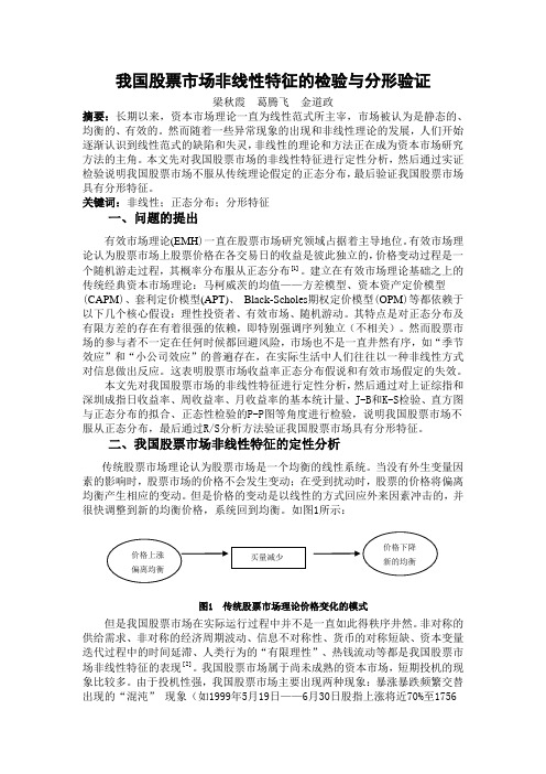
我国股票市场非线性特征的检验与分形验证梁秋霞葛腾飞金道政摘要:长期以来,资本市场理论一直为线性范式所主宰,市场被认为是静态的、均衡的、有效的。
然而随着一些异常现象的出现和非线性理论的发展,人们开始逐渐认识到线性范式的缺陷和失灵,非线性的理论和方法正在成为资本市场研究方法的主角。
本文先对我国股票市场的非线性特征进行定性分析,然后通过实证检验说明我国股票市场不服从传统理论假定的正态分布,最后验证我国股票市场具有分形特征。
关键词:非线性;正态分布;分形特征一、问题的提出有效市场理论(EMH)一直在股票市场研究领域占据着主导地位。
有效市场理论认为股票市场上股票价格在各交易日的收益是彼此独立的,价格变动过程是一个随机游走过程,其概率分布服从正态分布]1[。
建立在有效市场理论基础之上的传统经典资本市场理论:马柯威茨的均值——方差模型、资本资产定价模型(CAPM)、套利定价模型(APT)、Black-Scholes期权定价模型(OPM)等都依赖于以下几个核心假设:理性投资者、有效市场、随机游动。
其特点是对正态分布及有限方差的存在有着很强的依赖,即特别强调序列独立(不相关)。
然而股票市场的参与者不一定在任何时候都回避风险,市场也不是一直井然有序,如“季节效应”和“小公司效应”的普遍存在,在实际生活中人们往往以一种非线性方式对信息做出反应。
这表明股票市场收益率正态分布假说和有效市场假定的失效。
本文先对我国股票市场的非线性特征进行定性分析,然后通过对上证综指和深圳成指日收益率、周收益率、月收益率的基本统计量、J-B和K-S检验、直方图与正态分布的拟合、正态性检验的P-P图等角度进行检验,说明我国股票市场不服从正态分布,最后通过R/S分析方法验证我国股票市场具有分形特征。
二、我国股票市场非线性特征的定性分析传统股票市场理论认为股票市场是一个均衡的线性系统。
当没有外生变量因素的影响时,股票市场的价格不会发生变动;在受到扰动时,股票的价格将偏离均衡产生相应的变动。
Cubature Kalman Filters
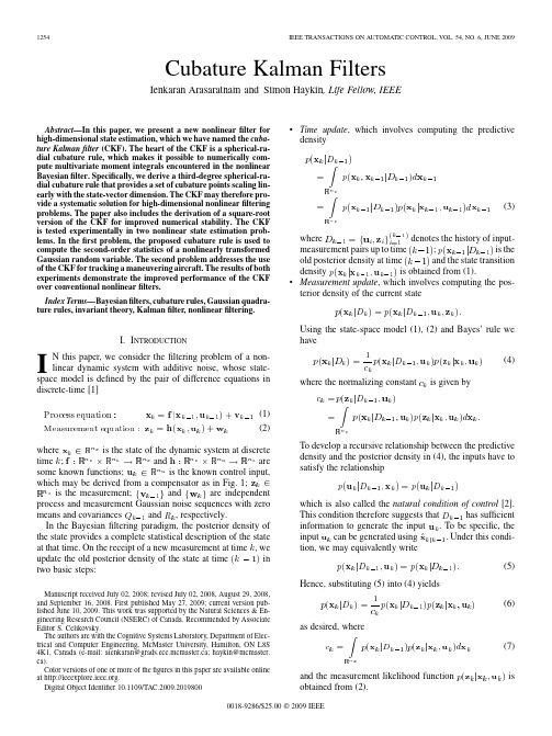
1254IEEE TRANSACTIONS ON AUTOMATIC CONTROL, VOL. 54, NO. 6, JUNE 2009Cubature Kalman FiltersIenkaran Arasaratnam and Simon Haykin, Life Fellow, IEEEAbstract—In this paper, we present a new nonlinear filter for high-dimensional state estimation, which we have named the cubature Kalman filter (CKF). The heart of the CKF is a spherical-radial cubature rule, which makes it possible to numerically compute multivariate moment integrals encountered in the nonlinear Bayesian filter. Specifically, we derive a third-degree spherical-radial cubature rule that provides a set of cubature points scaling linearly with the state-vector dimension. The CKF may therefore provide a systematic solution for high-dimensional nonlinear filtering problems. The paper also includes the derivation of a square-root version of the CKF for improved numerical stability. The CKF is tested experimentally in two nonlinear state estimation problems. In the first problem, the proposed cubature rule is used to compute the second-order statistics of a nonlinearly transformed Gaussian random variable. The second problem addresses the use of the CKF for tracking a maneuvering aircraft. The results of both experiments demonstrate the improved performance of the CKF over conventional nonlinear filters. Index Terms—Bayesian filters, cubature rules, Gaussian quadrature rules, invariant theory, Kalman filter, nonlinear filtering.• Time update, which involves computing the predictive density(3)where denotes the history of input; is the measurement pairs up to time and the state transition old posterior density at time is obtained from (1). density • Measurement update, which involves computing the posterior density of the current stateI. INTRODUCTIONUsing the state-space model (1), (2) and Bayes’ rule we have (4) where the normalizing constant is given byIN this paper, we consider the filtering problem of a nonlinear dynamic system with additive noise, whose statespace model is defined by the pair of difference equations in discrete-time [1] (1) (2)is the state of the dynamic system at discrete where and are time ; is the known control input, some known functions; which may be derived from a compensator as in Fig. 1; is the measurement; and are independent process and measurement Gaussian noise sequences with zero and , respectively. means and covariances In the Bayesian filtering paradigm, the posterior density of the state provides a complete statistical description of the state at that time. On the receipt of a new measurement at time , we in update the old posterior density of the state at time two basic steps:Manuscript received July 02, 2008; revised July 02, 2008, August 29, 2008, and September 16, 2008. First published May 27, 2009; current version published June 10, 2009. This work was supported by the Natural Sciences & Engineering Research Council (NSERC) of Canada. Recommended by Associate Editor S. Celikovsky. The authors are with the Cognitive Systems Laboratory, Department of Electrical and Computer Engineering, McMaster University, Hamilton, ON L8S 4K1, Canada (e-mail: aienkaran@grads.ece.mcmaster.ca; haykin@mcmaster. ca). Color versions of one or more of the figures in this paper are available online at . Digital Object Identifier 10.1109/TAC.2009.2019800To develop a recursive relationship between the predictive density and the posterior density in (4), the inputs have to satisfy the relationshipwhich is also called the natural condition of control [2]. has sufficient This condition therefore suggests that information to generate the input . To be specific, the can be generated using . Under this condiinput tion, we may equivalently write (5) Hence, substituting (5) into (4) yields (6) as desired, where (7) and the measurement likelihood function obtained from (2). is0018-9286/$25.00 © 2009 IEEEARASARATNAM AND HAYKIN: CUBATURE KALMAN FILTERS1255Fig. 1. Signal-flow diagram of a dynamic state-space model driven by the feedback control input. The observer may employ a Bayesian filter. The label denotes the unit delay.The Bayesian filter solution given by (3), (6), and (7) provides a unified recursive approach for nonlinear filtering problems, at least conceptually. From a practical perspective, however, we find that the multi-dimensional integrals involved in (3) and (7) are typically intractable. Notable exceptions arise in the following restricted cases: 1) A linear-Gaussian dynamic system, the optimal solution for which is given by the celebrated Kalman filter [3]. 2) A discrete-valued state-space with a fixed number of states, the optimal solution for which is given by the grid filter (Hidden-Markov model filter) [4]. 3) A “Benes type” of nonlinearity, the optimal solution for which is also tractable [5]. In general, when we are confronted with a nonlinear filtering problem, we have to abandon the idea of seeking an optimal or analytical solution and be content with a suboptimal solution to the Bayesian filter [6]. In computational terms, suboptimal solutions to the posterior density can be obtained using one of two approximate approaches: 1) Local approach. Here, we derive nonlinear filters by fixing the posterior density to take a priori form. For example, we may assume it to be Gaussian; the nonlinear filters, namely, the extended Kalman filter (EKF) [7], the central-difference Kalman filter (CDKF) [8], [9], the unscented Kalman filter (UKF) [10], and the quadrature Kalman filter (QKF) [11], [12], fall under this first category. The emphasis on locality makes the design of the filter simple and fast to execute. 2) Global approach. Here, we do not make any explicit assumption about the posterior density form. For example, the point-mass filter using adaptive grids [13], the Gaussian mixture filter [14], and particle filters using Monte Carlo integrations with the importance sampling [15], [16] fall under this second category. Typically, the global methods suffer from enormous computational demands. Unfortunately, the presently known nonlinear filters mentioned above suffer from the curse of dimensionality [17] or divergence or both. The effect of curse of dimensionality may often become detrimental in high-dimensional state-space models with state-vectors of size 20 or more. The divergence may occur for several reasons including i) inaccurate or incomplete model of the underlying physical system, ii) informationloss in capturing the true evolving posterior density completely, e.g., a nonlinear filter designed under the Gaussian assumption may fail to capture the key features of a multi-modal posterior density, iii) high degree of nonlinearities in the equations that describe the state-space model, and iv) numerical errors. Indeed, each of the above-mentioned filters has its own domain of applicability and it is doubtful that a single filter exists that would be considered effective for a complete range of applications. For example, the EKF, which has been the method of choice for nonlinear filtering problems in many practical applications for the last four decades, works well only in a ‘mild’ nonlinear environment owing to the first-order Taylor series approximation for nonlinear functions. The motivation for this paper has been to derive a more accurate nonlinear filter that could be applied to solve a wide range (from low to high dimensions) of nonlinear filtering problems. Here, we take the local approach to build a new filter, which we have named the cubature Kalman filter (CKF). It is known that the Bayesian filter is rendered tractable when all conditional densities are assumed to be Gaussian. In this case, the Bayesian filter solution reduces to computing multi-dimensional integrals, whose integrands are all of the form nonlinear function Gaussian. The CKF exploits the properties of highly efficient numerical integration methods known as cubature rules for those multi-dimensional integrals [18]. With the cubature rules at our disposal, we may describe the underlying philosophy behind the derivation of the new filter as nonlinear filtering through linear estimation theory, hence the name “cubature Kalman filter.” The CKF is numerically accurate and easily extendable to high-dimensional problems. The rest of the paper is organized as follows: Section II derives the Bayesian filter theory in the Gaussian domain. Section III describes numerical methods available for moment integrals encountered in the Bayesian filter. The cubature Kalman filter, using a third-degree spherical-radial cubature rule, is derived in Section IV. Our argument for choosing a third-degree rule is articulated in Section V. We go on to derive a square-root version of the CKF for improved numerical stability in Section VI. The existing sigma-point approach is compared with the cubature method in Section VII. We apply the CKF in two nonlinear state estimation problems in Section VIII. Section IX concludes the paper with a possible extension of the CKF algorithm for a more general setting.1256IEEE TRANSACTIONS ON AUTOMATIC CONTROL, VOL. 54, NO. 6, JUNE 2009II. BAYESIAN FILTER THEORY IN THE GAUSSIAN DOMAIN The key approximation taken to develop the Bayesian filter theory under the Gaussian domain is that the predictive density and the filter likelihood density are both Gaussian, which eventually leads to a Gaussian posterior den. The Gaussian is the most convenient and widely sity used density function for the following reasons: • It has many distinctive mathematical properties. — The Gaussian family is closed under linear transformation and conditioning. — Uncorrelated jointly Gaussian random variables are independent. • It approximates many physical random phenomena by virtue of the central limit theorem of probability theory (see Sections 5.7 and 6.7 in [19] for more details). Under the Gaussian approximation, the functional recursion of the Bayesian filter reduces to an algebraic recursion operating only on means and covariances of various conditional densities encountered in the time and the measurement updates. A. Time Update In the time update, the Bayesian filter computes the mean and the associated covariance of the Gaussian predictive density as follows: (8) where is the statistical expectation operator. Substituting (1) into (8) yieldsTABLE I KALMAN FILTERING FRAMEWORKB. Measurement Update It is well known that the errors in the predicted measurements are zero-mean white sequences [2], [20]. Under the assumption that these errors can be well approximated by the Gaussian, we write the filter likelihood density (12) where the predicted measurement (13) and the associated covariance(14) Hence, we write the conditional Gaussian density of the joint state and the measurement(15) (9) where the cross-covariance is assumed to be zero-mean and uncorrelated Because with the past measurements, we get (16) On the receipt of a new measurement , the Bayesian filter from (15) yielding computes the posterior density (17) (10) where is the conventional symbol for a Gaussian density. Similarly, we obtain the error covariance where (18) (19) (20) If and are linear functions of the state, the Bayesian filter under the Gaussian assumption reduces to the Kalman filter. Table I shows how quantities derived above are called in the Kalman filtering framework. The signal-flow diagram in Fig. 2 summarizes the steps involved in the recursion cycle of the Bayesian filter. The heart of the Bayesian filter is therefore how to compute Gaussian(11)ARASARATNAM AND HAYKIN: CUBATURE KALMAN FILTERS1257Fig. 2. Signal-flow diagram of the recursive Bayesian filter under the Gaussian assumption, where “G-” stands for “Gaussian-.”weighted integrals whose integrands are all of the form nonGaussian density that are present in (10), linear function (11), (13), (14) and (16). The next section describes numerical integration methods to compute multi-dimensional weighted integrals. III. REVIEW ON NUMERICAL METHODS FOR MOMENT INTEGRALS Consider a multi-dimensional weighted integral of the form (21) is some arbitrary function, is the region of where for all integration, and the known weighting function . In a Gaussian-weighted integral, for example, is a Gaussian density and satisfies the nonnegativity condition in the entire region. If the solution to the above integral (21) is difficult to obtain, we may seek numerical integration methods to compute it. The basic task of numerically computing the integral (21) is to find a set of points and weights that approximates by a weighted sum of function evaluations the integral (22) The methods used to find can be divided into product rules and non-product rules, as described next. A. Product Rules ), we For the simplest one-dimensional case (that is, may apply the quadrature rule to compute the integral (21) numerically [21], [22]. In the context of the Bayesian filter, we mention the Gauss-Hermite quadrature rule; when the is in the form of a Gaussian density weighting functionis well approximated by a polynomial and the integrand in , the Gauss-Hermite quadrature rule is used to compute the Gaussian-weighted integral efficiently [12]. The quadrature rule may be extended to compute multidimensional integrals by successively applying it in a tensorproduct of one-dimensional integrals. Consider an -point per dimension quadrature rule that is exact for polynomials of points for functional degree up to . We set up a grid of evaluations and numerically compute an -dimensional integral while retaining the accuracy for polynomials of degree up to only. Hence, the computational complexity of the product quadrature rule increases exponentially with , and therefore , suffers from the curse of dimensionality. Typically for the product Gauss-Hermite quadrature rule is not a reasonable choice to approximate a recursive optimal Bayesian filter. B. Non-Product Rules To mitigate the curse of dimensionality issue in the product rules, we may seek non-product rules for integrals of arbitrary dimensions by choosing points directly from the domain of integration [18], [23]. Some of the well-known non-product rules include randomized Monte Carlo methods [4], quasi-Monte Carlo methods [24], [25], lattice rules [26] and sparse grids [27]–[29]. The randomized Monte Carlo methods evaluate the integration using a set of equally-weighted sample points drawn randomly, whereas in quasi-Monte Carlo methods and lattice rules the points are generated from a unit hyper-cube region using deterministically defined mechanisms. On the other hand, the sparse grids based on Smolyak formula in principle, combine a quadrature (univariate) routine for high-dimensional integrals more sophisticatedly; they detect important dimensions automatically and place more grid points there. Although the non-product methods mentioned here are powerful numerical integration tools to compute a given integral with a prescribed accuracy, they do suffer from the curse of dimensionality to certain extent [30].1258IEEE TRANSACTIONS ON AUTOMATIC CONTROL, VOL. 54, NO. 6, JUNE 2009C. Proposed Method In the recursive Bayesian estimation paradigm, we are interested in non-product rules that i) yield reasonable accuracy, ii) require small number of function evaluations, and iii) are easily extendable to arbitrarily high dimensions. In this paper we derive an efficient non-product cubature rule for Gaussianweighted integrals. Specifically, we obtain a third-degree fullysymmetric cubature rule, whose complexity in terms of function evaluations increases linearly with the dimension . Typically, a set of cubature points and weights are chosen so that the cubature rule is exact for a set of monomials of degree or less, as shown by (23)Gaussian density. Specifically, we consider an integral of the form (24)defined in the Cartesian coordinate system. To compute the above integral numerically we take the following two steps: i) We transform it into a more familiar spherical-radial integration form ii) subsequently, we propose a third-degree spherical-radial rule. A. Transformation In the spherical-radial transformation, the key step is a change of variable from the Cartesian vector to a radius and with , so direction vector as follows: Let for . Then the integral (24) can be that rewritten in a spherical-radial coordinate system as (25) is the surface of the sphere defined by and is the spherical surface measure or the area element on . We may thus write the radial integral (26) is defined by the spherical integral with the unit where weighting function (27) The spherical and the radial integrals are numerically computed by the spherical cubature rule (Section IV-B below) and the Gaussian quadrature rule (Section IV-C below), respectively. Before proceeding further, we introduce a number of notations and definitions when constructing such rules as follows: • A cubature rule is said to be fully symmetric if the following two conditions hold: implies , where is any point obtainable 1) from by permutations and/or sign changes of the coordinates of . on the region . That is, all points in 2) the fully symmetric set yield the same weight value. For example, in the one-dimensional space, a point in the fully symmetric set implies that and . • In a fully symmetric region, we call a point as a generator , where if , . The new should not be confused with the control input . zero coordinates and use • For brevity, we suppress to represent a complete fully the notation symmetric set of points that can be obtained by permutating and changing the sign of the generator in all possible ways. Of course, the complete set entails where; are non-negative integers and . Here, an important quality criterion of a cubature rule is its degree; the higher the degree of the cubature rule is, the more accurate solution it yields. To find the unknowns of the cubature rule of degree , we solve a set of moment equations. However, solving the system of moment equations may be more tedious with increasing polynomial degree and/or dimension of the integration domain. For example, an -point cubature rule entails unknown parameters from its points and weights. In general, we may form a system of equations with respect to unknowns from distinct monomials of degree up to . For the nonlinear system to have at least one solution (in this case, the system is said to be consistent), we use at least as many unknowns as equations [31]. That is, we choose to be . Suppose we obtain a cu. In this case, we solve bature rule of degree three for nonlinear moment equations; the re) sulting rule may consist of more than 85 ( weighted cubature points. To reduce the size of the system of algebraically independent equations or equivalently the number of cubature points markedly, Sobolev proposed the invariant theory in 1962 [32] (see also [31] and the references therein for a recent account of the invariant theory). The invariant theory, in principle, discusses how to restrict the structure of a cubature rule by exploiting symmetries of the region of integration and the weighting function. For example, integration regions such as the unit hypercube, the unit hypersphere, and the unit simplex exhibit symmetry. Hence, it is reasonable to look for cubature rules sharing the same symmetry. For the case considered above and ), using the invariant theory, we may con( cubature points struct a cubature rule consisting of by solving only a pair of moment equations (see Section IV). Note that the points and weights of the cubature rule are in. Hence, they can be computed dependent of the integrand off-line and stored in advance to speed up the filter execution. where IV. CUBATURE KALMAN FILTER As described in Section II, nonlinear filtering in the Gaussian domain reduces to a problem of how to compute integrals, whose integrands are all of the form nonlinear functionARASARATNAM AND HAYKIN: CUBATURE KALMAN FILTERS1259points when are all distinct. For example, represents the following set of points:Here, the generator is • We use . set B. Spherical Cubature Rule. to denote the -th point from theWe first postulate a third-degree spherical cubature rule that takes the simplest structure due to the invariant theory (28) The point set due to is invariant under permutations and sign changes. For the above choice of the rule (28), the monomials with being an odd integer, are integrated exactly. In order that this rule is exact for all monomials of degree up to three, it remains to require that the rule is exact , 2. Equivalently, to for all monomials for which find the unknown parameters and , it suffices to consider , and due to the fully symmonomials metric cubature rule (29) (30) where the surface area of the unit sphere with . Solving (29) and (30) , and . Hence, the cubature points are yields located at the intersection of the unit sphere and its axes. C. Radial Rule We next propose a Gaussian quadrature for the radial integration. The Gaussian quadrature is known to be the most efficient numerical method to compute a one-dimensional integration [21], [22]. An -point Gaussian quadrature is exact and constructed as up to polynomials of degree follows: (31) where is a known weighting function and non-negative on ; the points and the associated weights the interval are unknowns to be determined uniquely. In our case, a comparison of (26) and (31) yields the weighting function and and , respecthe interval to be tively. To transform this integral into an integral for which the solution is familiar, we make another change of variable via yielding. The integral on the right-hand side of where (32) is now in the form of the well-known generalized GaussLaguerre formula. The points and weights for the generalized Gauss-Laguerre quadrature are readily obtained as discussed elsewhere [21]. A first-degree Gauss-Laguerre rule is exact for . Equivalently, the rule is exact for ; it . is not exact for odd degree polynomials such as Fortunately, when the radial-rule is combined with the spherical rule to compute the integral (24), the (combined) spherical-radial rule vanishes for all odd-degree polynomials; the reason is that the spherical rule vanishes by symmetry for any odd-degree polynomial (see (25)). Hence, the spherical-radial rule for (24) is exact for all odd degrees. Following this argument, for a spherical-radial rule to be exact for all third-degree polyno, it suffices to consider the first-degree genermials in alized Gauss-Laguerre rule entailing a single point and weight. We may thus write (33) where the point is chosen to be the square-root of the root of the first-order generalized Laguerre polynomial, which is orthogonal with respect to the modified weighting function ; subsequently, we find by solving the zeroth-order moment equation appropriately. In this case, we , and . A detailed account have of computing the points and weights of a Gaussian quadrature with the classical and nonclassical weighting function is presented in [33]. D. Spherical-Radial Rule In this subsection, we describe two useful results that are used to i) combine the spherical and radial rule obtained separately, and ii) extend the spherical-radial rule for a Gaussian weighted integral. The respective results are presented as two propositions: Proposition 4.1: Let the radial integral be computed numer-point Gaussian quadrature rule ically by theLet the spherical integral be computed numerically by the -point spherical ruleThen, an by-point spherical-radial cubature rule is given(34) Proof: Because cubature rules are devised to be exact for a subspace of monomials of some degree, we consider an integrand of the form(32)1260IEEE TRANSACTIONS ON AUTOMATIC CONTROL, VOL. 54, NO. 6, JUNE 2009where are some positive integers. Hence, we write the integral of interestwhereFor the moment, we assume the above integrand to be a mono. Making the mial of degree exactly; that is, change of variable as described in Section IV-A, we getWe use the cubature-point set to numerically compute integrals (10), (11), and (13)–(16) and obtain the CKF algorithm, details of which are presented in Appendix A. Note that the above cubature-point set is now defined in the Cartesian coordinate system. V. IS THERE A NEED FOR HIGHER-DEGREE CUBATURE RULES? In this section, we emphasize the importance of third-degree cubature rules over higher-degree rules (degree more than three), when they are embedded into the cubature Kalman filtering framework for the following reasons: • Sufficient approximation. The CKF recursively propagates the first two-order moments, namely, the mean and covariance of the state variable. A third-degree cubature rule is also constructed using up to the second-order moment. Moreover, a natural assumption for a nonlinearly transformed variable to be closed in the Gaussian domain is that the nonlinear function involved is reasonably smooth. In this case, it may be reasonable to assume that the given nonlinear function can be well-approximated by a quadratic function near the prior mean. Because the third-degree rule is exact up to third-degree polynomials, it computes the posterior mean accurately in this case. However, it computes the error covariance approximately; for the covariance estimate to be more accurate, a cubature rule is required to be exact at least up to a fourth degree polynomial. Nevertheless, a higher-degree rule will translate to higher accuracy only if the integrand is well-behaved in the sense of being approximated by a higher-degree polynomial, and the weighting function is known to be a Gaussian density exactly. In practice, these two requirements are hardly met. However, considering in the cubature Kalman filtering framework, our experience with higher-degree rules has indicated that they yield no improvement or make the performance worse. • Efficient and robust computation. The theoretical lower bound for the number of cubature points of a third-degree centrally symmetric cubature rule is given by twice the dimension of an integration region [34]. Hence, the proposed spherical-radial cubature rule is considered to be the most efficient third-degree cubature rule. Because the number of points or function evaluations in the proposed cubature rules scales linearly with the dimension, it may be considered as a practical step for easing the curse of dimensionality. According to [35] and Section 1.5 in [18], a ‘good’ cubature rule has the following two properties: (i) all the cubature points lie inside the region of integration, and (ii) all the cubature weights are positive. The proposed rule equal, positive weights for an -dimensional entails unbounded region and hence belongs to a good cubature family. Of course, we hardly find higher-degree cubature rules belonging to a good cubature family especially for high-dimensional integrations.Decomposing the above integration into the radial and spherical integrals yieldsApplying the numerical rules appropriately, we haveas desired. As we may extend the above results for monomials of degree less than , the proposition holds for any arbitrary integrand that can be written as a linear combination of monomials of degree up to (see also [18, Section 2.8]). Proposition 4.2: Let the weighting functions and be and . such that , we Then for every square matrix have (35) Proof: Consider the left-hand side of (35). Because a positive definite matrix, we factorize to be , we get Making a change of variable via is .which proves the proposition. For the third-degree spherical-radial rule, and . Hence, it entails a total of cubature points. Using the above propositions, we extend this third-degree spherical-radial rule to compute a standard Gaussian weighted integral as follows:ARASARATNAM AND HAYKIN: CUBATURE KALMAN FILTERS1261In the final analysis, the use of higher-degree cubature rules in the design of the CKF may marginally improve its performance at the expense of a reduced numerical stability and an increased computational cost. VI. SQUARE-ROOT CUBATURE KALMAN FILTER This section addresses i) the rationale for why we need a square-root extension of the standard CKF and ii) how the square-root solution can be developed systematically. The two basic properties of an error covariance matrix are i) symmetry and ii) positive definiteness. It is important that we preserve these two properties in each update cycle. The reason is that the use of a forced symmetry on the solution of the matrix Ricatti equation improves the numerical stability of the Kalman filter [36], whereas the underlying meaning of the covariance is embedded in the positive definiteness. In practice, due to errors introduced by arithmetic operations performed on finite word-length digital computers, these two properties are often lost. Specifically, the loss of the positive definiteness may probably be more hazardous as it stops the CKF to run continuously. In each update cycle of the CKF, we mention the following numerically sensitive operations that may catalyze to destroy the properties of the covariance: • Matrix square-rooting [see (38) and (43)]. • Matrix inversion [see (49)]. • Matrix squared-form amplifying roundoff errors [see (42), (47) and (48)]. • Substraction of the two positive definite matrices present in the covariant update [see (51)]. Moreover, some nonlinear filtering problems may be numerically ill-conditioned. For example, the covariance is likely to turn out to be non-positive definite when i) very accurate measurements are processed, or ii) a linear combination of state vector components is known with greater accuracy while other combinations are essentially unobservable [37]. As a systematic solution to mitigate ill effects that may eventually lead to an unstable or even divergent behavior, the logical procedure is to go for a square-root version of the CKF, hereafter called square-root cubature Kalman filter (SCKF). The SCKF essentially propagates square-root factors of the predictive and posterior error covariances. Hence, we avoid matrix square-rooting operations. In addition, the SCKF offers the following benefits [38]: • Preservation of symmetry and positive (semi)definiteness of the covariance. Improved numerical accuracy owing to the fact that , where the symbol denotes the condition number. • Doubled-order precision. To develop the SCKF, we use (i) the least-squares method for the Kalman gain and (ii) matrix triangular factorizations or triangularizations (e.g., the QR decomposition) for covariance updates. The least-squares method avoids to compute a matrix inversion explicitly, whereas the triangularization essentially computes a triangular square-root factor of the covariance without square-rooting a squared-matrix form of the covariance. Appendix B presents the SCKF algorithm, where all of the steps can be deduced directly from the CKF except for the update of the posterior error covariance; hence we derive it in a squared-equivalent form of the covariance in the appendix.The computational complexity of the SCKF in terms of flops, grows as the cube of the state dimension, hence it is comparable to that of the CKF or the EKF. We may reduce the complexity significantly by (i) manipulating sparsity of the square-root covariance carefully and (ii) coding triangularization algorithms for distributed processor-memory architectures. VII. A COMPARISON OF UKF WITH CKF Similarly to the CKF, the unscented Kalman filter (UKF) is another approximate Bayesian filter built in the Gaussian domain, but uses a completely different set of deterministic weighted points [10], [39]. To elaborate the approach taken in the UKF, consider an -dimensional random variable having with mean and covariance a symmetric prior density , within which the Gaussian is a special case. Then a set of sample points and weights, are chosen to satisfy the following moment-matching conditions:Among many candidate sets, one symmetrically distributed sample point set, hereafter called the sigma-point set, is picked up as follows:where and the -th column of a matrix is denoted ; the parameter is used to scale the spread of sigma points by from the prior mean , hence the name “scaling parameter”. Due to its symmetry, the sigma-point set matches the skewness. Moreover, to capture the kurtosis of the prior density closely, it is sug(Appendix I of [10], gested that we choose to be [39]). This choice preserves moments up to the fifth order exactly in the simple one-dimensional Gaussian case. In summary, the sigma-point set is chosen to capture a number as correctly as of low-order moments of the prior density possible. Then the unscented transformation is introduced as a method that are related to of computing posterior statistics of by a nonlinear transformation . It approximates the mean and the covariance of by a weighted sum of projected space, as shown by sigma points in the(36)(37)。
物理学百篇经典文献目录(125篇)

物理学百篇经典文献目录(125篇)1.Quantum Phase factors accompanying adiabatic changes, M. V. Berry, Proc. R.Soc. Lond. A, 392, 45-47 (1984).2.Significance of Electromagnetic Potentials in the Quantum Theory ,Y. Aharonovand Bohm D. Phys. Rev. 115, 485 (1959).3.Fate of the false vacuum. II. First quantum corrections ,Curtis G, Callan, Jr.andColeman S. Phys. Rev. D, 16, 1762, (1977).4.Theory of the condensation point, Langer J. S. , Ann. Phys. (N. Y. ) 41, 108(1967).5.Quantum tunnelling in a dissipative system, Caldeira A O and Leggett A J. Ann.Phys. (N. Y. ), 149, 374 (1983),6.Possible new effects in superconductors,Josephson B D,Phys. Lett. , 1, 251,(1962).7.The theory of a general quantum system interacting with a linear dissipativesystem Feynman R. P. and Vernon F L, Jr. Ann. Phys. (N.Y), 24, 118 (1963),8.Exact analysis of an interacting Bose gas, I. General solution and the groundstate, E. H. Lieb and W. Liniger, Phys. Rev. 130, 1605 (1963).9.Continuum dynamics of the 1-D Heisenberg antiferromagnet: Identification withthe O(3) nonlinear sigma model, Haldane F. D. M. Phys. Lett. A, 93, 464, (1983).10.Broken Symmetries, Goldstone J. Salam A and Weinberg S. Phys. Rev. , 127,965, (1962).11.Two solvable models of an antiferromagnetic chain, Lieb E, Schultz T andMattis D, Ann. Phys. (N. Y.) 16, 407, (1961).parison of quantum and semiclassical radiation theories with application tothe beam maser, Jaynes E T and Cummings F W. Proc. IEEE, 51 89 (1963).13.Reduction of a wave packet in quantum Brownian motion, Unruh W. G. andZurek W. H. Phys. Rev. D. 40 1071 (1989).14.Non-classical Properties of states generated by the excitations on a coherentstate, G. S. Agarwal and K. Tara, Phys. Rev. A, 43, 492, (1991).15.Relationship between Systems of Impenetrable Bosons and Fermions in OneDimension, M. Girardeau, J. Math. Phys. 1, 516, (1960).16.Divergence-free WKB theory, T. Hyouguchi, R. Seto, M. Ueda, S. Adachi, Annof Phys. 312 177-267 (2004).17.Fate of the false vacuum: Semi-classical theory, S. Coleman, Phys. Rev. D, 15,2929, 1977,18.Decay widths for metastable states: Improved WKB approximation, H. K.Shepard, Phys. Rev. D, 27, 1288, (1983)19.Solution of the one-dimensional electron gas on a lattice, V. J. Emery, A. Lutherand I. Peschel, Phys. Rev. B, 13, 1272, (1976).20.Luttinger liquid theory of one-dimensional quantum fluids: I. Properties of theLuttinger model and their extension to the general 1D interacting spinless Fermi gas, F. D. M. Haldane, J. Phys. C. Solid state Phys. 14, 2585, (1981).21.Spinor Bose Condensates in Optical Traps, T.-L. Ho, Phys. Rev. Lett. 81, 742(1998).22.Cold Bosonic Atoms in Optical Lattices, D. Jaksch, C. Bruder, J. I. Cirac, C. W.Gardiner, and P. Zoller, Phys. Rev. Lett. 81, 3108 (1998).23.Quantum Coherent Atomic Tunneling between Two Trapped Bose-EinsteinCondensates, A. Smerzi, S. Fantoni, S. Giovanazzi, and S. R. Shenoy, Phys. Rev.Lett. 79, 4950 (1997).24.Ground-State Properties of Magnetically Trapped Bose-Condensed RubidiumGas, G. Baym and C. J. Pethick, Phys. Rev. Lett. 76, 6 (1996).25.Observation of Bose-Einstein Condensation in a Dilute Atomic Vapor, M. H.Anderson, J. R. Ensher, M. R. Matthews, C. E. Wieman, and E. A. Cornell, Science 269, 198 (1995).26.Quantum Phase Transition from a Superfuid to a Mott Insulator in a Gas ofUltracold Atoms, M. Greiner, O. Mandel, T. Esslinger, T. W. Hänsch & I. Bloch, Nature (London) 415, 39 (2002).27.The General Solution and the Ground State, E. H. Lieb, W. Liniger, ExactAnalysis of an Interacting Bose Gas. I. Phys. Rev. 130, 1605 (1963).28.F. Dalfovo and S. Stringari, Bosons in Anisotropic Traps: Ground State andV ortices, F. Dalfovo and S. Stringari, Phys. Rev. A 53, 2477 (1996).29.Theory of Bose-Einstein Condensation in Trapped Gases, F. Dalfovo, S.Giorgini, L. P. Pitaevskii, and S. Stringari, Rev. Mod. Phys. 71, 463 (1999).30.Bose-Einstein Condensation in Dilute Gases, C. J. Pethick and H. Smith,(Cambridge, England, 2002).31.Can quantum-mechanical description of physical reality be consideredcomplete ,E.Einstein, B.Podolsky, and N.Rosen, Physical Review, 47:777-780(1935)32.Atom cooling trapping and quantum manipulation, C.E.Wieman, et al, Rew.Mod. Phys., 71, S253(1999)33.Quantum effects in one-photon and two-photon interference, L.Mandel, Rew.Mod. Phys. 71, S274 (1999)ser spectroscopy and quantum optics, T.W.Hansch and H.Walther, Rew. Mod.Phys., 71, S242 (1999)35.J.M.Raimond, M.Brune and S.Haroche, Colloquium:Manipulating quantumentanglement with atoms and photons in a cavity, Rew. Mod. Phys., 73, 565 (2001 )rmation and computation: Classical and quantum aspects, A.Galindo, et al,Rew. Mod. Phys.,, 74, 347(2002)37.Quantum cryptography, H.Zbinden, et al, Appl.Phys.B67,743(1998)38.Nobel Lecture: When atoms behave as waves: BEC and the atom laser,W.Ketterle, Rew. Mod. Phys., 74, 1131(2002)39.Nobel Lecture: BEC in a dilute gas, the first 70 years and some recentexperiments, E.A.Cornell and C.E.Wieman, Rew. Mod. Phys.., 74, 875(2002)40.Colloquium: Trapping and manipulating photon states in atomic ensembles,M.D.Lukin,Rew. Mod. Phys.,75, 457(2003)41.Nonclassical states in quantum optics: a squeezed review of the first 75 years,V.V.Dodonov, J. Opt. B, 4, R1-33(2002)42.Quantum nondemolition measurements: the route from toys to tools,V.B.Braginsky, et al, Rew. Mod. Phys., 68, 1-11(1996)43.Optical dipole traps for neutral atoms, R.Grimm and M.Weidemuller, arxiv:Physics /9902072(1999)44.Full observation of single-atom dynamics in cavity QED, H.Mabuchi, et al,quan-ph-9805076(1998)45.Single-photon sources,B. Lounis and M. Orrit, Rep. Prog. Phys. 68,1129-1179(2005)46.Focus on single photons on demand, P.Grangier, et al, special issue on NewJournal of Physics, 6, 1367-2630(2004)47.Quantum Information with Continuous Variables, Samuel Braunstein and Petervan Loock,Rew. Mod .Phys.,77,513(2005)48.From classical to quantum noise, Hermann A. Haus, J. Opt. Soc. Am. B12,2019(1995)49.Evidence for the quantum nature of light, D.F.Walls, Nuture,280, 451(1979)50.Electromagnetically induced transparency in ladder-type inhomogeneouslybroadened media: Theory and experiment, Julio Gea-Banacloche, Yong-qing Li, Shao-zheng Jin, and Min Xiao, Phys. Rev. A, 51,576-584(1995)51.Quantum-state transfer between fields and atoms in electromagnetically inducedtransparency, A.Dantan and M.Pinard, Phys. Rev. A69, 043810 (2004)52.Storage and retrival of single photons transmitted between remote quantummemories, T.Chaneliere, et al, Nature, 438, 833(2005)53.Measurement of dispersive properties of EIT in Rubidium atoms, Min Xiao, etal, Phys. Rev. Lett., 74, 666(1995)54.Observation of coherent optical information storage in an atomic medium usinghalted light pulses, C.Liu, et al, Nature, 409, 490(2001)55.Very cold trapped atoms ina vapor cell, C.Monroe, et al, Phys. Rev. Lett., 65,13,1571(1990)56.Observation of atoms laser cooled below the Doppler limit, P.D.Lett, et al, Phys.Rev. Lett.,61,169 (1988)57.Trapping of neutral sodium atoms with radiation pressure, E.L.Raab, et al, Phys.Rev. Lett., 59, 2631(1987)ing diode lasers for atomic physics, C.E.Wieman, Rev. Sci. Instrum, 62,1(1991)59.A narrow-band tunable diode laser system with grating feedback and a saturatedabsorption spectrometer for Cs and Rb, K.B.MacAdam, et al, Am J. Phys. 60, 1098(1992)60.Optical lattice: cold atoms ordered by light, L.Guidon and P.Verkerk, J. Opt. B,1, R23-R45(1999)61.Nobel Lecture: The manipulation of neutral particles, Steven Chu, Rev. Mod.Phys., 70, 685 - 706 (1998)62.Nobel Lecture: Laser cooling and trapping of neutral atoms , William D. Phillips,Rev. Mod. Phys., 70, 721 - 741 (1998)63.Nobel lecture: When atoms behave as waves: Bose-Einstein condensation andthe atom laser, Wolfgang Ketterle, Rev. Mod. Phys. 74, 1131 - 1151 (2002)64.Photoassociative Spectroscopy and Formation of Cold Molecules in ColdCesium Vapor: Trap–Loss Spectrum versus Ion Spectrum, Comparat D, Drag C, Fioretti A, et al. J. Mol. Spectrosc. 1999, 195: 229-23565.Long-range molecules and atomic scattering, Kevin M. Jones, Eite Tiesinga, PaulD. Lett, and Paul S. Julienne, Rev. Mod. Phys. V ol.78, April-June (2006)Experiments and theory in cold and ultracold collisions,John Weiner,Vanderlei S.Bagnato and Sergio Zilio,Paul S. Julienne, Rev. Mod. Phys. V ol.71, 1-84 (1999)66.Photoassociation of Ultracold Atoms: A New Spectroscopic. Technique, WilliamC. Stwalley and He Wang, J. Mol. Spectrosc. 1999, 195: 194-22867.Optical modification of a single impurity molecule in a solid, Basché, T., and W.E. Moerner. Nature. 1992. 355:335-337.68.Near-field spectroscopy of single molecules at room temperature, Trautman, J.K., J. J. Macklin, L. E. Brus, and E. Betzig. Sience. 1994. 369:40-42.69.Single-molecule spectroscopy: The road ahead, Orrit, M. J. Chem. Phys.2002.117: 10938-10946.70.Correlation between photons in two coherent beams of light, Hanbury Brown,R., and R. Q. Twiss. Nature. 1956.177:27-32.71.Photon statistics characterization of a single photon source, Alléaume, R., F.Treussart, J. M. Courty, and J. F. Roch. New J. Phys. 2004. 6:1-24.72.Quantum cryptography, N. Gisin, G. Ribordy, W. Tittel, Hugo Zbinden, Rev.Mod. Phys. 2002 , 74 14573.Direct measurement of the photo statistics of a triggered single photon source,F.Treussart, R. Alleaume, L.T.Xiao, et al. Phys. Rev. Lett. 2002, 89 09360174.Photoelectron spectroscopy without photoelectrons: Twenty years of ZEKEspectroscopy, Martin C. R. Cockett. Chem. Soc. Rev., 2005, 34, 935–94875.Chemical Applications of Zero Kinetic Energy (ZEKE) PhotoelectronSpectroscopy, Klaus Müller-Dethlefs and Edward W. Schlag. Angew. Chem. Int.Ed. 1998, 37, 1346 –13776.The spectroscopy of the Rydberg and ionic states of the I2–Arvan der Waalscomplexq, Martin C.R. Cockett. Journal of Electron Spectroscopy and Related Phenomena 97 (1998) 171–19077.Analysis of a quantum logic device based on dipole-dipole interactions ofoptically trapped Rydberg atoms , M. Saffman and T. G. Walker, Phys. Rev. A 72, 022347 (2005)78.Controlled many-body interactions in a frozen Rydberg gas, I. Mourachko,Wenhui Li, and T. F. Gallagher, Phys. Rev. A 70, 031401(R) (2004)79.Dipole Blockade at Förster Resonances in High Resolution Laser Excitation ofRydberg States of Cesium Atoms, Thibault V ogt, Matthieu Viteau, Jianming Zhao, Amodsen Chotia, Daniel Comparat, and Pierre Pillet, Phys. Rev. Lett. 97, 083003 (2006)80.Strongly coupled plasmas: high-density classical plasmas and degenerateelectron liquids, S. Ichimuru, Rev. Mod. Phys., 54(4):1017, 1982.81.Creation of an ultracold neutral plasma, T. C. Killian, S. Kulin, S. D. Bergeson,L. A. Orozco, C. Orzel, and S. L.Rolston, Phys. Rev. Lett.83 (23):4776, 1999.82.Ultracold Neutral Plasmas, T. C. Killian a, T. Pattard b, T. Pohl c and J. M,RostarXiv:physics/0612097v1 11 Dec 200683.A review of recent advances in semiconductor laser based gas monitors, P.Werle, Spectrochimica ACTA part A, 54, (1998) 197-23684.Spectroscopic trace gas analusis using semiconductor diode lasers, P. Werle,Spectrochimica ACTA part A, 52, (1996) 805-82285.Cavity ring-down spectroscopy: Experimental schemes and applications, BerdenG, Peeters R, Meijer G., Int. Reviews in Physical Chemistry, 19, (2000) 565-60786.Ultrasensitive frequency-modulation spectroscopy enhanced by a high-finesseoptical cavity: theory and application to overtone transitions of C2H2 and C2HD, L. S. Ma, J. Ye, P. Dube, and J. L. Hall, J. Opt. Soc. Am. B, 16, (1999) 2255-226887.原子核物理, 卢希庭主编, 胡济民审校,原子能出版社, 20088.原子核物理基础——核子与核, 宁平治, 李磊, 闵德芬,高等教育出版社,2003.89.粒子物理学(上), 章乃森编著,科学出版社, 1986. 粒子物理学(下), 章乃森编著, 科学出版社, 1987.90.正负电子物理, 唐孝威等,科学出版社, 199591.粒子物理与场论简引(中译本), T.D.Lee (李政道)著, 科学出版社.92.Elementary Particles, I.S. Hughes, Cambridge, 1972.93.Introduction to High Energy Physics, D.H. Perkins, Cambridge, 2000.94.Foundations of Quantum Chromodynamics, Z. Muta, World Scientific, 1987.95.Introduction to High Energy Physics, D.H. Perkins, Addison-Wesley PublishingCompany, 1986.96.Introduction to High-Energy Heavy-Ion Collisions, C.Y. Wong, World Scientific,1994.97.Gauge Theory of Elementary Particle Physics, Ta-Pei Cheng, Ling-Feng Li,Oxford, 198498.Thermal Field Theory, Cambridge, M.Le Bellae, 1996.99.Finite Temperature Field Theory, J.I. Kapusta, Cambridge, 1989.100.Relativistic Kinetic Theory, S.R.de Groot et al., North-Holland, 1980101.粒子物理实验方法, 唐孝威主编,高等教育出版社, 1982102.核与粒子物理实验方法, 王韶舜主编,原子能出版社, 1984103.原子核物理实验方法, 复旦大学, 清华大学, 北京大学合编, 原子能出版社, 1984.104.实验的数学处理, 李惕培,科学出版社, 1984.105.有关综述文献.106.Finite-difference time-domain analysis of an integrated circuit ceramic ball grid array package antenna for single-chip wireless transceivers, Y. P. Zhang, IEEE Transactions on Antennas and Propagation, V ol. 52, No. 2, 2004,435.107.Performance of inter-chip RF-interconnect using CPW, capacitive coupler and UWB transceivers, M. Sun, Y. P. Zhang, IEEE Transactions on Microwave Theory and Techniques, V ol. 53, No. 9, 2005, 2650.108.A derived physically expressive cicuit model for multilayer RF embedded passives, Jie Wang and Ke-Li Wu, IEEE Trans. Microwave Theory Tech., vol.54, no. 5, 2006, 1961.109.Analysis of the time response of nonuniform multiconductor transmission lines with a method of equivalent cascaded network chain, J. F. Mao and Z. F. Li, IEEE Transactions on Microwave Theory and Techniques, vol. 40, 1992. 948.110.Transmission line synthesis by the method of characteristics, J. F. Mao, O. Wing, and F. Y. Chang, IEEE Transactions on Circuits and System (Part I), vol. 43, 1996, 461.111.Theory and Experiment of Novel Microstrip Slow-Wave Open-Loop Resonator Filters, J. S. Hong, M. J. Lancaster, IEEE Trans. on Microwave Theory and Tech., vol. 45, no. 12, 1997, 2358.112.A low-pass prototype network for microwave linear phase filters, IEEE Trans.Microwave Theory Tech, J. D. Rhodes, vol. MTT-18, 1970, 290.113.Couplings of microstrip square openloop resonators for cross-coupled planar microwave filters, J. S. Hong and M. J. Lancaster, IEEE Trans. MicrowaveTheory Tech., vol. 44, 1996, 2099.114.A New Broadband Monolithic Passive Differential Coupler for K/Ka-Band Applications, IEEE Trans. Microwave Theory Tech, K. W. Hamed,A. P.Freundorfer, andY. M. Antar, vol. 54, no. 6, 2006, 2527.115.Novel Circuit Model for Three-Dimensional Geometries With Multilayer Dielectrics, IEEE Trans. Microwave Theory Tech, J. Jayabalan, B.L, Ooi, M.S. Leong, and M. K. Iyer, vol. 54, no. 4, 2006, 1331.116.50 Years Development of the Microwave Mixer for Heterodyne Reception, T. H.Oxley, I IEEE Trans. Microwave Theory Tech.,, vol. 50, no. 3, 2002, 867.117.Design of Microwave Filters, R. Levy,R. V. Snyder, and G. Matthaei,IEEE Trans. Microwave Theory Tech., vol. 50, no. 3, 2002, 783.118.Active Integrated Antennas, K. Chang, R. A. York, P. S. Hall, and T. Itoh, IEEE Trans. Microwave Theory Tech., vol. 50, no. 3, 2002, 937.119.Applications of RF/Microwaves in Medicine, A. Rosen, M. A. Stuchly, and A.V. Vorst, IEEE Trans. Microwave Theory Tech., vol. 50, no. 3, 2002, 963.120.Phased Arrays—Part I: Theory and Architectures, D. P. and David C.Zimmermann, IEEE Trans. Microwave Theory Tech., vol. 50, no. 3, 2002, 678.121.Propagation Prediction Models for Wireless Communication Systems, M. F.Iskander, and Z. Yun,IEEE Trans. Microwave Theory Tech., vol. 50, no. 3, 2002, 662.122.Biological Effects of Radio-Frequency/Microwave Radiation, E.R. Adair, and R.C. Petersen, IEEE Trans. Microwave Theory Tech., vol. 50, no. 3, 2002,953.123.Hybrid S-Parameters for Transmission Line Networks With Linear/Nonlinear Load Terminations Subject to Arbitrary Excitations, Y. Bayram,and J. L.Volakis, IEEE Trans. Microwave Theory Tech., vol. 55, no. 5, 2007,941.124.RF-System-On-Package (SOP) for Wireless Communications, K. Lim, et al, IEEE microwave magazine, March 2002, 88.125.A Compact Second-Order LTCC Bandpass Filter With Two Finite Transmission Zeros, L. K. Yeung, and K. L. Wu, IEEE Trans. Microwave Theory Tech., vol.51, no. 2, 2003,337.。
GeoStudio 系列软件在岩土工程中的应用-方法-技巧

中仿科技---专业信息化软件及技术咨询公司 CnTech Co.,Ltd--- Leading Engineering Virtual Prototyping Solutions Provider
info@
软件介绍
加拿大GEO-SLOPE 公司从 1977 年发展至今,已成为全球最大的 岩土软件开发公司之一,用户覆盖全球 100 多个国家。 中仿科技公司是GEO-SLOPE公司中国区独家区总代理商,希望 GEO-SLOPE公司的系列软件能给您的工作带来方便和帮助。 当您使用GeoStudio解决问题 时,您已经加入了遍布世界100多 个国家的工程师、大学教授、学 者和学生组成的群体。我们将一 如既往地致力于提高和加强软件 解决岩土工程问题的能力,使得 我们的软件功能更强大、更易于 使用。
CnTech Co.,Ltd--- Leading Engineering Virtual Prototyping Solutions Provider info@
• • • • 工程背景 几何模型 分析步骤 问题探讨
中仿科技---专业信息化软件及技术咨询公司 CnTech Co.,Ltd--- Leading Engineering Virtual Prototyping Solutions Provider
info@
•
SIGMA/W 的分析类型与本构模型
分析类型
Insitu Stress Redistribution Load/Deformation Coupled Stress/PWP Volume Change Dynamic Deformation
Effective-Drained Parameters Linear Elastic Anisotropic Elastic Hyperbolic NonlinearElastic Elastic-Plastic Soft Clay (MCC) Slip Surface Add-In Model Effective Parameters w/ PWP Change Linear Elastic Elastic-Plastic Soft Clay (MCC) Slip Surface Add-In Model
6 sigma 单词英文
A
Absolute deviation, 絕對離差 Absolute number, 絕對數 Absolute residuals, 絕對殘差 Acceleration array, 加速度立體陣 Acceleration in an arbitrary direction, 任意方向上的加速度 Acceleration normal, 法向加速度 Acceleration space dimension, 加速度空間的維數 Acceleration tangential, 切向加速度 Acceleration vector, 加速度向量 Acceptable hypothesis, 可接受假設 Accumulation, 累積 Accuracy, 準確度 Actual frequency, 實際頻數 Adaptive estimator, 自適應估計量 Addition, 相加 Addition theorem, 加法定理 Additivity, 可加性 Adjusted rate, 調整率 Adjusted value, 校正值 Admissible error, 容許誤差 Aggregation, 聚集性 Alternative hypothesis, 備擇假設 Among groups, 組間 Amounts, 總量 Analysis of correlation, 相關分析 Analysis of covariance, 協方差分析 Analysis of regression, 回歸分析 Bar chart, 條形圖 Bar graph, 條形圖 Base period, 基期 Bayes' theorem , Bayes定理 Bell-shaped curve, 鍾形曲線 Bernoulli distribution, 伯努力分佈 Best-trim estimator, 最好切尾估計量 Bias, 偏性 Binary logistic regression, 二元邏輯斯蒂回歸 Binomial distribution, 二項分佈 Analysis of time series, 時間序列分析 Analysis of variance, 方差分析 Angular transformation, 角轉換 ANOVA (analysis of variance), 方差分析 ANOVA Models, 方差分析模型 Arcing, 弧/弧旋 Arcsine transformation, 反正弦變換 Area under the curve, 曲線面積 AREG , 評估從一個時間點到下一個時間點回歸相關時的誤差 ARIMA, 季節和非季節性單變數模型的極大似然估計 Arithmetic grid paper, 算術格紙 Arithmetic mean, 算術平均數 Arrhenius relation, 艾恩尼斯關係 Assessing fit, 擬合的評估 Associative laws, 結合律 Asymmetric distribution, 非對稱分佈 Asymptotic bias, 漸近偏倚 Asymptotic efficiency, 漸近效率 Asymptotic variance, 漸近方差 Attributable risk, 歸因危險度 Attribute data, 屬性資料 Attribution, 屬性 Autocorrelation, 自相關 Autocorrelation of residuals, 殘差的自相關 Average, 平均數 Average confidence interval length, 平均置信區間長度 Average growth rate, 平均增長率
- 1、下载文档前请自行甄别文档内容的完整性,平台不提供额外的编辑、内容补充、找答案等附加服务。
- 2、"仅部分预览"的文档,不可在线预览部分如存在完整性等问题,可反馈申请退款(可完整预览的文档不适用该条件!)。
- 3、如文档侵犯您的权益,请联系客服反馈,我们会尽快为您处理(人工客服工作时间:9:00-18:30)。
ǫ k c† ck + J
k <i,j>
Si · Sj + K
i
Si · Sc (ri ) (1)
2 where J, K > 0, are the Heisenberg and Kondo coupling respectively, and Sc (ri ) = c† i,α σαβ ci,α . Since we are interested in the AFM phase, the Heisenberg term can be mapped onto the non-linear sigma model in a well-known manner [22]. The local spin, Si = (−1)i n + 1 , has both |S |l a Neel component, n, and a small ferromagnetic moment, l ∝ ∂τ n × n. The conduction electrons couple to both the Neel vector, Sc (ri ) · n, and also the ferromagnetic part of the local spin, Sc (ri ) · l. Upon integrating out the electrons, we obtain two 4th order terms, one due to the coupling to the Neel component and the other to the ferromagnetic part. As we have assumed a Fermi surface that is not nested by the AF wave vector, (π, π ), there is a kinetic energy gap for the former term. Similarly, there are no low-lying fermionic excitations that couple to n to give rise to Landau damping; hence it remains a z = 1 theory. The effective Lagrangian in terms of the Goldstone modes, π a , where a ∈ x, y is,
PACS numbers:
The physics of heavy-fermion metals, systems that contain both localized f -electrons and conduction electron bands, has been of great interest in the stronglycorrelated community for several decades. Initial work by Doniach [1] pointed out the competition between the Kondo (JK ) and the RKKY (JH ) interaction, and the quantum critical point (QCP) associated with the transition from an antiferromagnetic metal (AFM) to a paramagnetic (PM) state as JK and JH vary. Work on the two-impurity model [2, 3] showed that the RKKY and Kondo coupling are not mutually exclusive either for ferromagnetic or antiferromagnetic interactions. In fact, a correlated Kondo effect is the rule rather than the exception, with the impurities partially compensated by the conduction electrons, and partially by each other (for AF interactions). In 1-D, there have been various numerical [4] and analytical [5, 6] studies. However, the physics of higher dimensional systems and the corresponding quantum phase transition (QPT) is much less well-understood. A commonly assumed scenario is that the f -electrons delocalize and are included in the Fermi surface, resulting in a large Fermi surface as given by Luttinger’s Theorem [7, 8], and the QPT is of the spin density-wave (SDW) type. This QPT has typically been understood in the Hertz-Millis approach [9, 10], and the physics of delocalized f -electrons forming a heavy fermi liquid have been well-understood in a large-N approach [11, 12, 13]. However, experimental studies have shown that the HertzMillis picture may be inadequate for describing the behavior of the system near the QCP [14, 15]. An alternative picture of the AFM to PM transition is that the f electrons do not delocalize and become part of the Fermi surface, hence the Fermi surface is small. This picture has been proposed by several groups [16, 17], and studied within the DMFT approach [16, 18]. Exotic ground states have also been proposed for Kondo lattice systems [19, 20, 21] that include fractionalized quasi-particles. We study the effect of the Kondo coupling on the antiferromagnetic phase transition, and also see if the various exotic states can be obtained from a more microscopic
Nonlinear Sigma Model Analysis of the AFM Phase Transition of the Kondo Lattice
T. Tzen Ong1, 2 and B. A. Jones2
1 2
Department of Applied Physics, Stanford University, Stanford CA 94305, USA IBM Research Division, Almaden Research Center, San Jose, CA 95120, USA (Dated: August 27, 2008)
approach. We assume that the AFM state has a small Fermi surface, with no“hot-spots” spanned by the Neel vector (π, π ), as shown in Fig. 1. Tom of Fermi surface with no “hot”-spots nested by Q = (π, π ). The solid black lines indicate the Fermi surface, and the dashed black lines indicate the magnetic B.Z. .
QPT of the two-dimensional (2D) square Kondo lattice with a small Fermi surface, we map the system onto a non-linear sigma model (NLSM) coupled to conduction electrons. We then obtain an effective Lagrangian by integrating out the fermionic degrees of freedom, and carry out a renormalization group (RG) analysis to one-loop within the ǫ-expansion. The calculations and results are described in the following sections. As we shall show, there is a new QCP, with logarithmic scaling due to the Kondo interaction that plays an essential role in the QPT. The Kondo interaction strongly affects the spin-wave fluctuations near the QCP, and leads to logarithmic scaling of the spin-wave velocity, implying localization of the spin-waves due to the Kondo effect. Based upon the RG results, we also propose a possible phase diagram near the AFM state. The Hamiltonian for the Kondo-Heisenberg model is written as: H=