Optimal Tuning of PI Speed Controller Using Nature Inspired
执行器饱和下的最优 IMC-PI控制器设计

执行器饱和下的最优 IMC-PI控制器设计夏浩;于明莉;李柳柳;杨希珞【期刊名称】《计算机应用研究》【年(卷),期】2016(33)4【摘要】控制器性能会受到执行器饱和现象的影响,为了准确评价系统在出现执行器饱和时的跟踪性能,研究了饱和条件下基于内模法(internal model control,IMC)的跟踪性能基准PI控制器的设计问题。
当被控对象可近似为一阶带滞后(first order plus dead time,FOPDT)模型时,选取绝对误差积分(integral absolute error,IAE)为控制器性能评价指标,给出了IAE指标与控制器参数的关系。
通过分析闭环传递函数的时域特性,建立控制器输出最大值与控制器参数的解析关系,可直接根据解析关系式选取饱和情形下基准IMC-PI控制器的参数。
仿真证明所提方法较其他抗饱和方法更为简洁且跟踪效果更好。
%Actuator saturation can affect the performance of PI controller.In order to assess the setpoint tracking performance under actuator saturation accurately,the paper studied the design method of PI controller based on internal model control (IMC)with optimal setpiont tracking performance.With the plant approximated to the first order plus time delay (FOPDT) model,the control performance index used the integral absolute error (IAE),this paper developed the relationship between IAE index and controller parameter.By analyzing the time-response of closed-loop transfer function,the paper established the analytic relationship between the maximum controller output and the controller tuning parameter.Based on this relationship,selecting the optimal IMC-PI controller under actuator saturation is more simple.Simulation experiments show that the design method in this paper is more concise and has better setpoint tracking performance than other common anti-windup methods.【总页数】4页(P1083-1086)【作者】夏浩;于明莉;李柳柳;杨希珞【作者单位】大连理工大学电子信息与电气工程学部,辽宁大连 116024;大连理工大学电子信息与电气工程学部,辽宁大连 116024;大连理工大学电子信息与电气工程学部,辽宁大连 116024;大连理工大学电子信息与电气工程学部,辽宁大连 116024【正文语种】中文【中图分类】TP273.2【相关文献】1.具有执行器饱和系统的控制器设计理论及应用研究 [J], 方敏;孙秀丽;方会2.考虑执行器饱和约束的非光滑船舶航向控制器设计 [J], 王国峰;郑凯;王兴成3.具有非线性执行器饱和的时滞切换系统的控制器设计 [J], 张美玉;刘玉忠4.一体化执行器饱和线性矩阵不等式跟踪容错控制器设计 [J], 刘聪;钱坤;李颖晖;刘勇智;丁奇5.小电容应用下的三角形联结级联H桥STATCOM建模和最优控制器设计 [J], 王恒宜;汪飞因版权原因,仅展示原文概要,查看原文内容请购买。
先进的PID控制
北京化工大学本科毕业论文题目:基于遗传算法整定的PID控制院系:专业:电气工程及其自动化班级:________ ____ _ _ _____ 学生姓名:____________ ________ _____ 执导老师:___________ ______________ ______论文提交日期:年月日论文答辩日期:年月日摘要PID控制器是在工业过程控制中常见的一种控制器,因此,PID参数整定与优化一直是自动控制领域研究的重要问题。
遗传算法是一种具有极高鲁棒性的全局优化方法,在自控领域得到广泛的应用。
针对传统PID 参数整定的困难性,本文提出了把遗传算法运用于PID参数整定中。
本文首先对PID控制的原理和PID参数整定的方法做了简要的介绍。
其次介绍了遗传算法的原理、特点和应用。
再次,本文结合实例阐述了基于遗传算法的PID参数优化方法,采用误差绝对值时间积分性能指标作为参数选择的最小目标函数,利用遗传算法的全局搜索能力,使得在无须先验知识的情况下实现对全局最优解的寻优,以降低PID参数整定的难度,达到总体上提高系统的控制精度和鲁棒性的目的。
最后,本文针对遗传算法收敛速度慢、易早熟等缺点,将传统的赌盘选择法与最优保存策略结合起来,并采用改进的自适应交叉算子和自适应变异算子对PID参数进行迭代寻优整定。
采用MATLAB对上述算法进行仿真验证,仿真结果表明了遗传算法对PID参数整定的有效性。
关键词:PID;参数控制;遗传算法;MATLABAbstractPID controller is a kind of controller that is usual in industrial process control. Therefore, tuning and optimization of PID parameters are important researchable problems in the automatic control field, where Genetic algorithm is widely used because of the highly robust global optimization ability of it. Aiming at the difficulty of traditional tuning of PID parameter, this paper puts forward a method that genetic algorithm is applied to the tuning of PID parameters.Firstly, the principle of PID control and the methods of tuning of PID parameters are introduced briefly. Secondly, this paper introduces the principle, characteristics and application of genetic algorithm. Thirdly, this article expounds on the methods of tuning of PID parameters based on genetic algorithm with an example. In this paper, the performance index of time integral of absolute error serves as the minimum objective function in the tuning of PID parameters, and the global search ability of genetic algorithm is used, so the global optimal solution is obtained without prior knowledge, and the difficulty of tuning of PID parameter is reduced, so the goal is achieved which is improving the control accuracy and robustness of the system overall. Finally, aiming at the weakness of genetic algorithm, such as the slow convergence of prematurity and precocious, the traditional gambling site selection method and elitist model are united in this paper, and the paper alsoadopted adaptive crossover operator and adaptive mutation operator to optimize PID parameters iteratively.Use MATLAB to simulate these algorithms, and the simulation results show that PID controller tuning based on genetic algorithm is effective.Keywords: Genetic algorithm; PID control; optimum; MATLAB目录第一章引言 (1)1.1 课题研究的背景及意义 (1)1.2 PID控制的发展与现状 (1)1.3 本文研究的内容 (2)第二章PID控制 (4)2.1 PID控制原理 (4)2.2 常规PID参数整定方法 (6)2.2.1 Ziegler-Nichols整定方法 (6)2.2.2 改进的Ziegler-Nichols整定方法 (8)2.2.3 ISTE最优设定方法的经验公式 (9)2.2.4 Haalman法的计算公式 (10)2.2.5 KT整定法 (11)第三章基于遗传算法整定的PID控制 (13)3.1 遗传算法基本原理 (13)3.1.1 遗传算法概要 (13)3.1.2 遗传算法的应用步骤 (14)3.2 遗传算法的实现 (15)3.2.1 编码方法 (15)3.2.2 适应度函数 (16)3.2.3 选择算子 (17)3.2.4 交叉算子 (17)3.2.5 变异算子 (18)3.2.6 遗传算法控制参数选取 (19)3.3 遗传算法的仿真验证 (20)3.2.6遗传算法中关键参数的确定 (23)3.3 遗传算法的主要步骤 (23)3.3.1 准备工作 (23)3.3.2 基本遗传算法的步骤 (24)3.4遗传算法PID参数整定的编程实现 (24)3.4.1初始群体 (24)3.4.2 编码 (25)3.4.3 基本操作算子 (26)3.4.4 目标函数 (29)3.4.5 画图 (29)第四章PID整定方法的仿真应用 (31)4.1 一阶对象 (31)4.2 二阶对象 (32)4.3 三阶对象 (34)第五章结论 (37)参考文献 (38)致谢 (40)第一章引言1.1 课题研究的背景及意义PID(p一proportion,I一Integral,D一Differentia)控制是比例、积分、微分控制的简称PID[l]。
PID controller
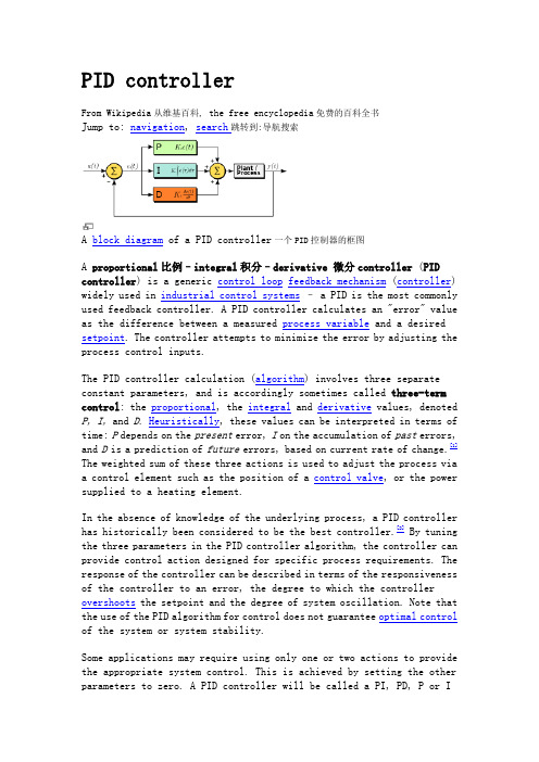
PID controller免费的百科全书Jump to: navigation, search跳转到:导航搜索A block diagram of a PID controller一个PID控制器的框图A proportional比例–integral积分–derivative 微分controller (PID controller) is a generic control loop feedback mechanism (controller) widely used in industrial control systems– a PID is the most commonly used feedback controller. A PID controller calculates an "error" value as the difference between a measured process variable and a desired setpoint. The controller attempts to minimize the error by adjusting the process control inputs.The PID controller calculation (algorithm) involves three separate constant parameters, and is accordingly sometimes called three-term control: the proportional, the integral and derivative values, denoted P,I, and D.Heuristically, these values can be interpreted in terms of time: P depends on the present error, I on the accumulation of past errors, and D is a prediction of future errors, based on current rate of change.[1] The weighted sum of these three actions is used to adjust the process via a control element such as the position of a control valve, or the power supplied to a heating element.In the absence of knowledge of the underlying process, a PID controller has historically been considered to be the best controller.[2] By tuning the three parameters in the PID controller algorithm, the controller can provide control action designed for specific process requirements. The response of the controller can be described in terms of the responsiveness of the controller to an error, the degree to which the controller overshoots the setpoint and the degree of system oscillation. Note that the use of the PID algorithm for control does not guarantee optimal control of the system or system stability.Some applications may require using only one or two actions to provide the appropriate system control. This is achieved by setting the other parameters to zero. A PID controller will be called a PI, PD, P or Icontroller in the absence of the respective control actions. PI controllers are fairly common, since derivative action is sensitive to measurement noise, whereas the absence of an integral term may prevent the system from reaching its target value due to the control action.Contents[hide]∙ 1 Control loop basics∙ 2 PID controller theoryo 2.1 Proportional term2.1.1 Droopo 2.2 Integral termo 2.3 Derivative term∙ 3 Loop tuningo 3.1 Stabilityo 3.2 Optimum behavioro 3.3 Overview of methodso 3.4 Manual tuningo 3.5 Ziegler–Nichols methodo 3.6 PID tuning software∙ 4 Modifications to the PID algorithm∙ 5 History∙ 6 Limitations of PID controlo 6.1 Linearityo 6.2 Noise in derivative∙7 Improvementso7.1 Feed-forwardo7.2 Other improvements∙8 Cascade control∙9 Physical implementation of PID control∙10 Alternative nomenclature and PID formso10.1 Ideal versus standard PID formo10.2 Basing derivative action on PVo10.3 Basing proportional action on PVo10.4 Laplace form of the PID controllero10.5 PID Pole Zero Cancellationo10.6 Series/interacting formo10.7 Discrete implementationo10.8 Pseudocode∙11 PI controller∙12 See also∙13 References∙14 External linkso14.1 PID tutorialso14.2 Special topics and PID control applications [edit] Control loop basics基本控制回路Further information更多信息: Control system控制系统A familiar example of a control loop is the action taken when adjusting hot and cold faucets (valves) to maintain the water at a desired temperature. This typically involves the mixing of two process streams, the hot and cold water. The person touches the water to sense or measure its temperature. Based on this feedback they perform a control action to adjust the hot and cold water valves until the process temperature stabilizes at the desired value.The sensed water temperature is the process variable or process value (PV). The desired temperature is called the setpoint (SP). The input to the process (the water valve position) is called the manipulated variable (MV). The difference between the temperature measurement and the set point is the error (e) and quantifies whether the water is too hot or too cold and by how much.After measuring the temperature (PV), and then calculating the error, the controller decides when to change the tap position (MV) and by how much. When the controller first turns the valve on, it may turn the hot valve only slightly if warm water is desired, or it may open the valve all the way if very hot water is desired. This is an example of a simple proportional control. In the event that hot water does not arrive quickly, the controller may try to speed-up the process by opening up the hot water valve more-and-more as time goes by. This is an example of an integral control.Making a change that is too large when the error is small is equivalent to a high gain controller and will lead to overshoot. If the controller were to repeatedly make changes that were too large and repeatedly overshoot the target, the output would oscillate around the setpoint in either a constant, growing, or decaying sinusoid. If the oscillations increase with time then the system is unstable, whereas if they decrease the system is stable. If the oscillations remain at a constant magnitude the system is marginally stable.In the interest of achieving a gradual convergence at the desired temperature (SP), the controller may wish to damp the anticipated future oscillations. So in order to compensate for this effect, the controller may elect to temper its adjustments. This can be thought of as a derivative control method.If a controller starts from a stable state at zero error (PV = SP), then further changes by the controller will be in response to changes in other measured or unmeasured inputs to the process that impact on the process, and hence on the PV. Variables that impact on the process other than the MV are known as disturbances. Generally controllers are used to reject disturbances and/or implement setpoint changes. Changes in feedwater temperature constitute a disturbance to the faucet temperature control process.In theory, a controller can be used to control any process which has a measurable output (PV), a known ideal value for that output (SP) and an input to the process (MV) that will affect the relevant PV. Controllers are used in industry to regulate temperature, pressure, flow rate, chemical composition, speed and practically every other variable for which a measurement exists.[edit] PID controller theoryThis section describes the parallel or non-interacting form of the PID controller. For other forms please see the section Alternative nomenclature and PID forms.The PID control scheme is named after its three correcting terms, whose sum constitutes the manipulated variable (MV). The proportional, integral, and derivative terms are summed to calculate the output of the PIDcontroller. Defining as the controller output, the final form of the PID algorithm is:where: Proportional gain, a tuning parameter: Integral gain, a tuning parameter: Derivative gain, a tuning parameter: Error: Time or instantaneous time (the present) [edit] Proportional termPlot of PV vs time, for three values of Kp (Kiand Kdheld constant)The proportional term makes a change to the output that is proportional to the current error value. The proportional response can be adjusted by multiplying the error by a constant K p, called the proportional gain.The proportional term is given by:A high proportional gain results in a large change in the output for a given change in the error. If the proportional gain is too high, the system can become unstable (see the section on loop tuning). In contrast, a small gain results in a small output response to a large input error, and a less responsive or less sensitive controller. If the proportional gain is too low, the control action may be too small when responding to system disturbances. Tuning theory and industrial practice indicate that the proportional term should contribute the bulk of the output change.[citation needed][edit] DroopA pure proportional controller will not always settle at its target value, but may retain a steady-state error. Specifically, drift in the absence of control, such as cooling of a furnace towards room temperature, biases a pure proportional controller. If the drift is downwards, as in cooling, then the bias will be below the set point, hence the term "droop".Droop is proportional to the process gain and inversely proportional to proportional gain. Specifically the steady-state error is given by:Droop is an inherent defect of purely proportional control. Droop may be mitigated by adding a compensating bias term (setting the setpoint above the true desired value), or corrected by adding an integral term.[edit] Integral termPlot of PV vs time, for three values of Ki (Kpand Kdheld constant)The contribution from the integral term is proportional to both the magnitude of the error and the duration of the error. The integral in a PID controller is the sum of the instantaneous error over time and gives the accumulated offset that should have been corrected previously. Theaccumulated error is then multiplied by the integral gain () and added to the controller output.The integral term is given by:The integral term accelerates the movement of the process towards setpoint and eliminates the residual steady-state error that occurs with a pure proportional controller. However, since the integral term responds to accumulated errors from the past, it can cause the present value to overshoot the setpoint value (see the section on loop tuning).[edit] Derivative termPlot of PV vs time, for three values of Kd (Kpand Kiheld constant)The derivative of the process error is calculated by determining the slope of the error over time and multiplying this rate of change by thederivative gain . The magnitude of the contribution of the derivative term to the overall control action is termed the derivative gain, . The derivative term is given by:The derivative term slows the rate of change of the controller output. Derivative control is used to reduce the magnitude of the overshoot produced by the integral component and improve the combinedcontroller-process stability. However, the derivative term slows thetransient response of the controller. Also, differentiation of a signal amplifies noise and thus this term in the controller is highly sensitive to noise in the error term, and can cause a process to become unstable if the noise and the derivative gain are sufficiently large. Hence an approximation to a differentiator with a limited bandwidth is more commonly used. Such a circuit is known as a phase-lead compensator.[edit] Loop tuningTuning a control loop is the adjustment of its control parameters (proportional band/gain, integral gain/reset, derivative gain/rate) to the optimum values for the desired control response. Stability (bounded oscillation) is a basic requirement, but beyond that, different systems have different behavior, different applications have different requirements, and requirements may conflict with one another.PID tuning is a difficult problem, even though there are only three parameters and in principle is simple to describe, because it must satisfy complex criteria within the limitations of PID control. There are accordingly various methods for loop tuning, and more sophisticated techniques are the subject of patents; this section describes some traditional manual methods for loop tuning.Designing and tuning a PID controller appears to be conceptually intuitive, but can be hard in practice, if multiple (and often conflicting) objectives such as short transient and high stability are to be achieved. Usually, initial designs need to be adjusted repeatedly through computer simulations until the closed-loop system performs or compromises as desired.Some processes have a degree of non-linearity and so parameters that work well at full-load conditions don't work when the process is starting up from no-load; this can be corrected by gain scheduling (using different parameters in different operating regions). PID controllers often provide acceptable control using default tunings, but performance can generally be improved by careful tuning, and performance may be unacceptable with poor tuning.[edit] StabilityIf the PID controller parameters (the gains of the proportional, integral and derivative terms) are chosen incorrectly, the controlled process input can be unstable, i.e., its output diverges, with or withoutoscillation, and is limited only by saturation or mechanical breakage. Instability is caused by excess gain, particularly in the presence of significant lag.Generally, stabilization of response is required and the process must not oscillate for any combination of process conditions and setpoints, though sometimes marginal stability (bounded oscillation) is acceptable or desired.[citation needed][edit] Optimum behaviorThe optimum behavior on a process change or setpoint change varies depending on the application.Two basic requirements are regulation (disturbance rejection – staying at a given setpoint) and command tracking(implementing setpoint changes) –these refer to how well the controlled variable tracks the desired value. Specific criteria for command tracking include rise time and settling time. Some processes must not allow an overshoot of the process variable beyond the setpoint if, for example, this would be unsafe. Other processes must minimize the energy expended in reaching a new setpoint.[edit] Overview of methodsThere are several methods for tuning a PID loop. The most effective methods generally involve the development of some form of process model, then choosing P, I, and D based on the dynamic model parameters. Manual tuning methods can be relatively inefficient, particularly if the loops have response times on the order of minutes or longer.The choice of method will depend largely on whether or not the loop can be taken "offline" for tuning, and the response time of the system. If the system can be taken offline, the best tuning method often involves subjecting the system to a step change in input, measuring the output as a function of time, and using this response to determine the control parameters.Choosing a Tuning MethodMethod Advantages DisadvantagesManual Tuning No math required. Online method. Requires experienced personnel.Ziegler–Nichols Proven Method. Online method. Process upset, sometrial-and-error, veryaggressive tuning.Software Tools Consistent tuning. Online oroffline method. May includevalve and sensor analysis. Allow simulation before downloading. Can support Non-Steady State(NSS) Tuning.Some cost and training involved.Cohen-Coon Good process models. Some math. Offline method. Only good forfirst-order processes.[edit ] Manual tuningIf the system must remain online, one tuning method is to first set and values to zero. Increase the until the output of the loop oscillates, then the should be set to approximately half of that valuefor a "quarter amplitude decay" type response. Then increaseuntil any offset is corrected in sufficient time for the process. However, too muchwill cause instability. Finally, increase , if required, until the loop is acceptably quick to reach its reference after a load disturbance. However, too much will cause excessive response and overshoot. A fast PID loop tuning usually overshoots slightly to reach the setpoint more quickly; however, some systems cannot accept overshoot, in which case an over-damped closed-loop system is required, which will require a setting significantly less than half that of the setting causing oscillation. Effects of increasing a parameter independently Parameter Rise time OvershootSettlingtime Steady-state error Stability [3] Decrease Increase Smallchange DecreaseDegrade Decrease [4] Increase Increase Decrease DegradesignificantlyMinor decrease Minor decrease Minor decrease No effect intheory Improve if small[edit ] Ziegler –Nichols methodFor more details on this topic, see Ziegler –Nichols method .Another heuristic tuning method is formally known asthe Ziegler –Nichols method , introducedbyJohnG.ZieglerandNathaniel B. Nichols in the 1940s. As in the method above, the and gains are first set to zero. TheP gain is increased until it reaches the ultimate gain,, at which the output of the loop starts to oscillate.and the oscillation periodare used to set the gains as shown:Ziegler –Nichols methodControl Type P- - PI-PID These gains apply to the ideal, parallel form of the PID controller. When applied to the standard PID form, the integral and derivative time parameters and are only dependent on the oscillation period . Please see the section "Alternative nomenclature and PID forms ".[edit ] PID tuning softwareMost modern industrial facilities no longer tune loops using the manual calculation methods shown above. Instead, PID tuning and loopoptimization software are used to ensure consistent results. These software packages will gather the data, develop process models, andsuggest optimal tuning. Some software packages can even develop tuning by gathering data from reference changes.Mathematical PID loop tuning induces an impulse in the system, and then uses the controlled system's frequency response to design the PID loop values. In loops with response times of several minutes, mathematical loop tuning is recommended, because trial and error can take days just to find a stable set of loop values. Optimal values are harder to find. Some digital loop controllers offer a self-tuning feature in which very small setpoint changes are sent to the process, allowing the controller itself to calculate optimal tuning values.Other formulas are available to tune the loop according to different performance criteria. Many patented formulas are now embedded within PID tuning software and hardware modules.Advances in automated PID Loop Tuning software also deliver algorithms for tuning PID Loops in a dynamic or Non-Steady State (NSS) scenario. The software will model the dynamics of a process, through a disturbance, and calculate PID control parameters in response.[edit] Modifications to the PID algorithmThe basic PID algorithm presents some challenges in control applications that have been addressed by minor modifications to the PID form.Integral windupFor more details on this topic, see Integral windup.One common problem resulting from the ideal PID implementations is integral windup, where a large change in setpoint occurs (say a positive change) and the integral term accumulates an error larger than the maximal value for the regulation variable (windup), thus the system overshoots and continues to increase as this accumulated error is unwound. This problem can be addressed by:∙Initializing the controller integral to a desired value∙Increasing the setpoint in a suitable ramp∙Disabling the integral function until the PV has entered the controllable region∙Limiting the time period over which the integral error is calculated ∙Preventing the integral term from accumulating above or below pre-determined boundsOvershooting from known disturbancesFor example, a PID loop is used to control the temperature of an electric resistance furnace, the system has stabilized. Now the door is opened and something cold is put into the furnace thetemperature drops below the setpoint. The integral function of the controller tends to compensate this error by introducing another error in the positive direction. This overshoot can be avoided by freezing of the integral function after the opening of the door for the time the control loop typically needs to reheat the furnace. Replacing the integral function by a model based partOften the time-response of the system is approximately known. Then it is an advantage to simulate this time-response with a model and to calculate some unknown parameter from the actual response of the system. If for instance the system is an electrical furnace the response of the difference between furnace temperature and ambient temperature to changes of the electrical power will be similar to that of a simple RC low-pass filter multiplied by an unknownproportional coefficient. The actual electrical power supplied to the furnace is delayed by a low-pass filter to simulate the response of the temperature of the furnace and then the actual temperature minus the ambient temperature is divided by this low-pass filtered electrical power. Then, the result is stabilized by anotherlow-pass filter leading to an estimation of the proportionalcoefficient. With this estimation, it is possible to calculate the required electrical power by dividing the set-point of thetemperature minus the ambient temperature by this coefficient. The result can then be used instead of the integral function. This also achieves a control error of zero in the steady-state, but avoids integral windup and can give a significantly improved controlaction compared to an optimized PID controller. This type ofcontroller does work properly in an open loop situation which causes integral windup with an integral function. This is an advantage if, for example, the heating of a furnace has to be reduced for some time because of the failure of a heating element, or if thecontroller is used as an advisory system to a human operator who may not switch it to closed-loop operation. It may also be useful if the controller is inside a branch of a complex control system that may be temporarily inactive.Many PID loops control a mechanical device (for example, a valve). Mechanical maintenance can be a major cost and wear leads to control degradation in the form of either stiction or a deadband in the mechanical response to an input signal. The rate of mechanical wear is mainly a function of how often a device is activated to make a change. Where wearis a significant concern, the PID loop may have an output deadband to reduce the frequency of activation of the output (valve). This is accomplished by modifying the controller to hold its output steady if the change would be small (within the defined deadband range). The calculated output must leave the deadband before the actual output will change.The proportional and derivative terms can produce excessive movement in the output when a system is subjected to an instantaneous step increase in the error, such as a large setpoint change. In the case of the derivative term, this is due to taking the derivative of the error, which is very large in the case of an instantaneous step change. As a result, some PID algorithms incorporate the following modifications:Derivative of the Process VariableIn this case the PID controller measures the derivative of themeasured process variable (PV), rather than the derivative of the error. This quantity is always continuous (i.e., never has a step change as a result of changed setpoint). For this technique to be effective, the derivative of the PV must have the opposite sign of the derivative of the error, in the case of negative feedbackcontrol.Setpoint rampingIn this modification, the setpoint is gradually moved from its old value to a newly specified value using a linear or first orderdifferential ramp function. This avoids the discontinuity present in a simple step change.Setpoint weightingSetpoint weighting uses different multipliers for the errordepending on which element of the controller it is used in. The error in the integral term must be the true control error to avoidsteady-state control errors. This affects the controller'ssetpoint response. These parameters do not affect the response to load disturbances and measurement noise.[edit] HistoryThis section requires expansion.PID theory developed by observing the action of helmsmen.PID controllers date to 1890s governor design.[2][5] PID controllers were subsequently developed in automatic ship steering. One of the earliest examples of a PID-type controller was developed by Elmer Sperry in 1911,[6] while the first published theoretical analysis of a PID controller was by Russian American engineer Nicolas Minorsky, in (Minorsky 1922). Minorsky was designing automatic steering systems for the US Navy, and based his analysis on observations of a helmsman, observing that the helmsman controlled the ship not only based on the current error, but also on past error and current rate of change;[7]this was then made mathematical by Minorsky. His goal was stability, not general control, which significantly simplified the problem. While proportional control provides stability against small disturbances, it was insufficient for dealing with a steady disturbance, notably a stiff gale (due to droop), which required adding the integral term. Finally, the derivative term was added to improve control.Trials were carried out on the USS New Mexico, with the controller controlling the angular velocity (not angle) of the rudder. PI control yielded sustained yaw (angular error) of ±2°, while adding D yielded yaw of ±1/6°, better than most helmsmen could achieve.[8]The Navy ultimately did not adopt the system, due to resistance by personnel. Similar work was carried out and published by several others in the 1930s.[edit] Limitations of PID controlWhile PID controllers are applicable to many control problems, and often perform satisfactorily without any improvements or even tuning, they can perform poorly in some applications, and do not in general provide optimal control. The fundamental difficulty with PID control is that it is a feed back system, with constant parameters, and no direct knowledge of the process, and thus overall performance is reactive and a compromise –while PID control is the best controller with no model of the process,[2] better performance can be obtained by incorporating a model of the process.The most significant improvement is to incorporate feed-forward control with knowledge about the system, and using the PID only to control error. Alternatively, PIDs can be modified in more minor ways, such as by changing the parameters (either gain scheduling in different use cases or adaptively modifying them based on performance), improving measurement (higher sampling rate, precision, and accuracy, and low-pass filtering if necessary), or cascading multiple PID controllers.PID controllers, when used alone, can give poor performance when the PID loop gains must be reduced so that the control system does not overshoot, oscillate or hunt about the control setpoint value. They also have difficulties in the presence of non-linearities, may trade-off regulation versus response time, do not react to changing process behavior (say, the process changes after it has warmed up), and have lag in responding to large disturbances.[edit] LinearityAnother problem faced with PID controllers is that they are linear, and in particular symmetric. Thus, performance of PID controllers innon-linear systems (such as HVAC systems) is variable. For example, in temperature control, a common use case is active heating (via a heating element) but passive cooling (heating off, but no cooling), so overshoot can only be corrected slowly –it cannot be forced downward. In this case the PID should be tuned to be overdamped, to prevent or reduce overshoot, though this reduces performance (it increases settling time).[edit] Noise in derivativeA problem with the derivative term is that small amounts of measurement or process noise can cause large amounts of change in the output. It is often helpful to filter the measurements with a low-pass filter in order to remove higher-frequency noise components. However, low-pass filtering and derivative control can cancel each other out, so reducing noise by instrumentation is a much better choice. Alternatively, a nonlinear median filter may be used, which improves the filtering efficiency and practical performance.[9]In some case, the differential band can be turned off in many systems with little loss of control. This is equivalent to using the PID controller as a PI controller.。
蚁群算法在PID参数优化中的应用研究

第8卷 第5期 中 国 水 运 Vol.8 No.5 2008年 5月 China Water Transport May 2008收稿日期:2008-03-30作者简介:李楠,浙江海洋学院机电工程学院。
蚁群算法在PID 参数优化中的应用研究李 楠,胡即明(浙江海洋学院 机电工程学院,浙江 舟山 316000)摘 要:本文介绍了蚁群算法的基本原理,将蚁群算法应用到了PID 控制的参数优化问题中,并详细给出了基于蚁群算法的PID 控制参数优化算法的实现步骤。
为了验证本文算法的可行性,我们对文献[1]中的例子进行了仿真,并将仿真结果与文献[1]给出的基于遗传算法的PID 控制参数优化结果进行了比较,发现:基于蚁群算法的PID 参数优化算法无论是在最优解的质量方面还是在算法的执行效率方面都要优于基于遗传算法的PID 参数优化算法。
关键词:蚁群算法;PID 控制;遗传算法;信息素中图分类号:TP301.6 文献标识码:A 文章编号:1006-7973(2008)05-0101-03一、引言在控制系统中,PID (比例-积分-微分)控制是控制器最常用的控制规律。
PID 控制早在20世纪30年代末期就已经出现,但由于其具有算法简单、鲁棒性好及可靠性高等优点,所以在控制工程领域里至今还是具有很强的生命力。
在PID 控制中,PID 参数K p ,T i 和T d 的整定是决定整个PID 控制系统性能优劣的关键环节。
因此,PID 参数的整定和优化问题一直倍受人们的关注。
在过去的几十年里,已经形成了一系列的PID 参数优化算法。
如,经典的Ziegler—Nichols (ZN)[2]算法,基于遗传算法的PID 参数优化设计[3]等。
其中,基于遗传算法的PID 参数优化设计是一种利用仿生优化算法对PID 控制进行参数优化的设计方法,这是一种全新的设计思想,已经逐渐成为PID 应用领域中的一个新的研究内容。
另一方面,蚁群优化是Marco Dorigo 等学者在真实蚂蚁觅食行为的启发下提出的一种具有高度创新性的元启发式算法[4]。
一类多输入多输出系统的预测PID控制算法仿真

计算量也大为减少 , 从而提高了控制算法的有效性和可行 性。
1 系统描述和 γ GPC 算法
考虑如下离散差分方程描述的
( )
−1
p -输入 / p -输出的多
(1)
变量系统 A( z − 1 ) ∆y (k ) = z −1 B (z −1 )∆ u (k ) + ζ (k ) 其中 u (k ) 和 y (k ) 分别为包含 量
• 496 •
系
统
仿
真
学
报 注
Vol. 16 No. 3 March. 2004 性能指标(7)的右端前两项为标准 GPC 的性能指
定问题,提出了一种介于 GPC 和 PID 之间的折中算法。这 种算法的优点是既保留了预测控制的长处, 同时又考虑了操 作人员所熟悉的 PID 参数的调节方法。另外,这里采用了 一类改进的 GPC 算法,即所谓的 γ GPC ,这使得所需的
( )
L
A p z −1
( )}
(3)
将上式写为矢量形式
= GU + f
Y = GU + H z − 1 ∆ u (k − 1 ) + F z − 1 y (k )
( )
( )
其中 Ai z
( ) 为最高阶次二阶的标量多项式,其形式如下
( )
B1,1 z − 1 −1 B z = 2,1 M B p,1 z −1
用于实际工业过程的控制 [1]。即使在先进控制策略层出不穷 的今天,PID 控制仍然以其结构简单、调整维护方便、算法 简洁明了和操作人员易于接受而占据着过程控制中的主导 地位,因而使得几乎所有的工业控制系统都把 PID 控制作 为标准的控制算法。 但是,PID 控制在处理过程具有时滞、非最小相位或非 常规的动态特性时,在性能上会受到很大的限制。而对于更 加复杂的系统,就不得不采用先进的控制策略,例如:广义 预测控制( GPC)[2]、动态矩阵控制(DMC)[3]等来获得更 好的控制性能。虽然,这类先进的预测控制算法能够提供更 高级的控制, 但是也存在多种原因阻碍着它在实际场合中的 应用。 其中一个主要的原因就是由于这类先进的控制算法在 硬件、软件和人员培训方面缺乏有效的支持,阻碍了它在 DCS 层上的实现,而且在参数调节方面,由于这类先进控
新型模糊PID控制及在HVAC系统的应用

新型模糊PID控制及在HV AC系统的应用第26卷第11期2009年11月控制理论与应用ControlTheory&Applications文章编号:1000—8152(2009)11—1277—05新型模糊PID控制及在HV AC系统的应用吕红丽,段培永,崔玉珍,贾磊z(1.山东建筑大学信息与电气工程学院,山东济南250101;2.山东大学控制科学与工程学院,山东济南250061)摘要:为了推广模糊控制器在非线性系统中的应用,提出一种利用PID控制器的参数优化和调节模糊控制器的新糊控制器设计算法,然后利用改进的变论域思想进一步优化模糊控制器设计参数.将其应用于暖通空调(HV AC)系统的节能控制中并与常规PID控制器相比较,仿真和实验结果表明这种模糊控制器具有超调量小,跟踪迅速,鲁棒性强等优越的控制性能.关键词:模糊控制;PID控制;结构分析;变论域;暖通空调系统中图分类号:TP273文献标识码:A NovelfuzzyPIDcontrolandapplicationtoHV ACsystemsLOHong.1i,DUANPei—yong,CUIYu.zhen,JIALei(rmationandElectricalEngineeringCollege,ShandongJianzhuUniversity,JinanSha ndong250101,China;2.SchoolofControlScienceandEngineering,ShandongUniversity,JinanShandong250061,China)Abstract:Inordertoextendtheapplicationoffuzzycontrollertononlinearsystems,anewfuzz ycontrolstrategytrollerandthelineargainoftheconventionalPIDcontrollerisderivedbasedonthegtructurean alysisoffuzzycontroller~—tuninginthePIDcontroller~Furthermore,theimprovedvariableuniversemethodisemployedtooptimizetheparametertuni ngofthefuzzycontrolleron—savingcontrolinheating,ventilating,andair—conditioning(HV AC)thatthisfuzzycontrolleriseffectiveandthealgorithmprovideslessovershoot,shortersetting timeandbetterrobustness,etc.Keywords:fuzzycontrol;PIDcontrol;structureanalysis;variableuniverse;HV ACsystems 1引言(Introduction)自1974年Mamdani将模糊控制首次应用到蒸汽机车的控制以来[1],基于Zadeh提出的模糊逻辑技术发展起来的模糊控制已经被成功应用到各种过程作经验而无需建立系统的精确数学模型,但模糊控制器仍无法在现实工业过程中大范围的进行推广和应用,主要原因之一是现场操作人员难以理解和掌前工业过程中大部分控制问题所面临的是高度非线性,时变,含有扰动等不确定性因素的复杂非线性规PID控制器仍然被广泛应用,但是由于实际被控过程的复杂性往往很难获得满意的控制效果[4].尽管收稿日期:2008-01一lO;收修改稿日期:2009—02--03 基金项目:山东省自然科学基金资助项目(Z2006G07); 很多先进的控制技术已经被用来调节和改进PID控制器的设计【516],但是这些并不能改变PID控制器本行逆向思维,尝试探索模糊控制器与PID控制器的一种新型的组合设计形式,利用成熟的PID控制器增益因子对模糊控制器的参数进行设计和调节,提出了一种基于PID控制器增益因子的模糊控制器新型设计方法.这样既充分利用PID控制器的成熟技术,同时又发挥了模糊控制器的全局非线性优势,提高控制系统的鲁棒性,还使得模糊控制技术便于普通技术人员的学习和掌握.'2模糊控制器的结构和参数设计(Structure andparametersdesignoffuzzycontroller)考虑一个通常的闭环反馈控制系统,其中r,u和控制理论与应用第26卷先经过分析和比较确定采用输入变量均为e,Ae,输出变量分别为直接输出饥和增量输出Au的2维模糊控制器的并联组合,即采用模糊PD控制器uPD:F1(e,△e),和模糊PI控制器△PI=(e,△e).模糊控制器的参数可通过设计参数和调节参数两部分进定,同时所有变量均采用基本论域为f-1,11,并且把在卜1,1】上完成设计参数的模糊控制器称为通用模正规化因子即可完成整个模糊控制器的设计过程.2.1通用模糊控制器的设计(Designofnominal fuzzycontrollers)考虑模糊PD控制器(e,Ae),在任意给定的采样时刻n,e(n),△e)作为控制器的输入变量,u(礼)作为控制器的输出,模糊控制器结构参数具体设计如下:e,△e(礼)首先通过正规化因子Ge】,GAe】进行正规化变换转换到基本论域上,u(n)的正规化因子为Gu,即e*=,Gei.e(n),△e=G△?△e(竹)j(1)(佗)=Gu.这里i=1,2且e,Ae,,Au∈『-1,11.两个输入变量e,Ae的隶属函数如图1所示,每一个变量存在两个模糊集合,分别记作JF)e,Ne,PAe,NAe,输出变量的模糊集合乱采用模糊单点集,本文考虑e,Ae,u∈『一1,1】,并且采用线性模糊规则,模糊and运算选用算术积product;模糊or运算选用有界和算子sum;模糊蕴涵运算选择取小算子min;解模糊算法选择加权平均法.N(£)P/\一一l01e图1输入变量e的隶属函数Fig.1Themembershipfunctionofinpute{2.2通用模糊控制器的结构分析(Sructureanaly—sisofnominalfuzzycontrollers1为了基于PID控制器参数设计模糊控制器,首先必须通过模糊控制器的结构分析获得两者之间的解析关系,继续考虑模糊PD控制器(e,Ae),在采样时刻礼,e(礼),△e(礼)进入模糊控制系统,经过模糊推理过程,解模糊以及反正规化变换得到局部输出结果:u1=Gu?札木=Gu(e+Ae,)/2=Gu(Cel?e(n)+GAel?△e(礼))/2.(2)对于平行结构的增量模糊控制器F2(e,Ae),选择与F1相同设计参数的通用模糊控制器,只是其输出变量是Au,,正规化因子为Ge2,GAe2,GAu,经过结构分析得到其局部模糊控制器输出为Au2=GAu?Au=GAu(eAe)/2=GAu(Ge2?e(n)+GAe2?Ae(n))/2.(3)系(AnalyticalrelationbetweenfuzzyandPID controllers)基于以上的模糊控制器的结构解析分析考虑常规PID控制器与模糊控制器的参数之间的解析关系并选取Gel=Ge2=Ge,GAe1=GAe2=GAe.(4)于是全局模糊控制器的输出为fuyn)=l+∑Au2=(Ge.e(n)+G△e.Ae(n))+(Ge.e(叩)+GAe.△e(叩)):言[(Gu?Ge+GAu?GAe)?e(n)+Gu?GAe?Ae(n)+GAu?Ge?∑e(叩)】.(5)为了与常规PID控制器相对应,选择Kp:=G(a△Uu'.+2△u'G△/6于是"lZfuzzy(n)=Kp?e(n)+KI∑e(i)+?△e(n).(7)模糊控制律(7)在n采样时刻形式上完全成为一种常规PID控制器,但是随着时间的变化,,/co3个增益系数也随之不断变化,实现了一组特殊PID控常规PID控制器的增益系数,,KD是已知常数,并与所设计的模糊控制器在n采样时刻对应相等,把第11期吕红丽等:新型模糊PID控制及在HV AC系统的应用1279 fGAe=(Kp-t-,//郦一4‰)?Ge/2硒,《Gu=4KDKI/(Kp土,//郦-4KIKD)Ge,(8)IGAu=/Ge.可见模糊控制器和常规PID控制器之间存在着精确的解析关系,于是模糊控制器与常规PID控制器可以通过以上的解析关系式来设计模糊控制器的正规化因子.3基于PID控制参数的模糊控制器新型设计(Noveldesignoffuzzycontrollersbased—onPIDparameters)器(Noveldesignoffuzzycontrollersbased—on conventionalPIDparameters)首先设计出系统的常规PID控制器,获得其比的初始正规化因子Ge0保持不变,于是初步确定误步分析调节PID控制器的增益系数来间接调节模糊增加时,输出响应加速,而稳态误差也会降低,但是当太大时会引起震荡或者不稳定.此时,根据解析关系(8),对应的GAe的值随着增加而增加,Gu随着增加而减小,代替了简单的比例因子的单一变化.同理,当PID控制器中的积分因子增加时,GAe随着积分因子增加而减小,而Gu和GAu的增加反应了两个局部并行模糊控制器各自规则输出的变化;当PID控制器中的微分因子KD增加时, 降低稳态误差同时加速系统响应,GAe随着微分因子KD增加而减小,Gu增加而GAu保持不变.数优化(Parameteroptimizationoffuzzycon—trollersbased-onimprovedvariableuniverse)模糊控制器的积分环节有时候在平衡点附近会产生一些细微的连续震荡,消除震荡的一种改进论域本质是改变变量的正规化因子,因此如果通用模糊控制器的论域保持不变,那么通过增加模糊控制器输入变量的正规化因子的取值同样达到了缩小论域的目的,从而优化了模糊控制器的规则.将以上设计得到的模糊控制器正规化因子分别记作GAe.,Gu0,GAu.,当误差变得很小时继续缩小论域来优化控制性能,于是适当的放大输出误差正规化因子Ge,对模糊控制器参数在平衡点附近进行细微的调节,完成模糊控制系统的参数在线优化,实现在误差较小时的高精度模糊控制,从而进一步提高模糊控制系统性能.4仿真结果(Simulationresults)为了验证模糊控制器新型设计算法的有效性,过程G(s)=_0.3e-O.8~.(9)首先设计出常规PID控制器:u(n)=一1.875?e(礼)一2.08?∑e(v)+0.09Ae(n).然后选取适合于被控对象的参数和算法设计出通用模糊控制器,采用第3节的设计选定初始正规化误差因子Ge0=l,模糊控制器的调节参数为△u=2.08.最后将以上设计的模糊控制器作用于系统f9),基于变论域思想在线调节模糊控制器的各个正规化制器分别作用于控制系统(9),可以看到它们的控制输出响应几乎是相同的,如图2所示,这说明针对被控对象保持不变的系统,设计的模糊控制器具有常规PID控制器同样的控制性能.,FC一…PID一图22O406080100tlS被控过程(9)的系统响应曲线Controlresponseofprocess(9)5模糊控制在暖通空调中的应用研究(ApplyfuzzycontrollersintoHV ACsys一针对暖通空调系统的空气处理机组设计控制器,个物理回路,强迫对流的热交换过程非常复杂,很得PID控制器的参数和实现模糊控制器设计,把经过热交换后进入房间之前的空气温度,回风机的干球温度.作为空调处理机组的输出变量,而冷冻水的1280控制理论与应用第26卷流速h是可操作变量,假设进入蒸发器的冷冻水温度hi是常数,水流速是根据空调房间的冷冻.=.厂(.h,,i,hwi),(10)其中,表示系统的非线性时变函数,在稳定状态下以及很小的区间上可采用下面的模型进行较准确的估计:0(s)Kchwe一…,—TFtchw(8)一'儿J这里:h,h,Lh分别是冷冻水的过程增益,时间常数,时间滞后,它们是随着空气和水的控制器设计的有效性.考虑方程(11)所描述的热交换过程,在不同的操作区域内进行高,中,低3种不器,得到增益系数,KI,KD分别为1.1,1.22和0.09,基于这3个参数设计出相应的模糊控制器,然后分别作用于对3种工况下的系统,得到图4的PID控制和模糊控制结果.室夕一一图3空气处理机组的结构图.--FC...设定值一nnn'一一低中高一0l00200300400500600t|S-i.低.'中图4模糊控制与PID控制的输出响应仿真结果表明,最初根据PID控制器参数设计的模糊控制器对第1种工况的控制效果很理想,但是当模型发生变化时,PID控制器和模糊控制器的参数都保持不变的情况下,PID控制器很难适应模型变化, 系统震荡强烈,第3种工况时系统几乎无法稳定,而过仿真试验的验证后将该新型模糊控制设计方法应用到HV AC实验室系统的空气处理机组的温度控制是固定不变的,测量信号包括水和空气的流速,空气和水的温度,而且冷负荷的变化是通过空气和水的实验结果.图中表明与常规PID控制器相比,模糊控制器跟踪迅速,超调时间短,稳定性好,具有较强的鲁棒性.t}S图5模糊控制器与PID控制器的实验结果6结语(Conclusion)为了更好的研究非线性系统的复杂控制问题,推广模糊控制器的应用,使模糊控制器的设计更加简单实用,本文提出一种利用PID控制器的增益因子仅尝试着将模糊控制器的结构分析这一理论研究成果推广到模糊控制器的应用领域,而且充分利用了常规PID控制器的成熟经验.仿真和实验结果表明,这种模糊控制器的新型设计具有良好的控制性能.参考文献(References):…namicplant[J].InstitutionofElectricalEngineers,1974,121(12): 1585——1588.systemsanddecisionprocesses[J].IEEETransactionsonSystems, ManandCybernetic,1973,3(1):28—44.应用,2008,25(4):780—782.05O5O5O5O50的""第11期吕红丽等:新型模糊PID控制及在HV AC系统的应用1281 nonlinearsystems[J].ControlTheory&Applications,2008,25(4): 780—782.)制.控制理论与应用,2008,25(3):468—474.—ternbasedonsupportvectormachines[J].ControlTheory&Applica—tions,2008,25(4):468—474.)[5】BIQ,CAIWJ,WANGQG,eta1.Advancedcontrollerauto?tuning anditsapplicationinHV ACsystems[J].ControlEngineeringPrac—tice,2000,8(3):633—644.—PIDcontrollerwithoptimalfuzzyreasoning[J].IEEETransactionsonSystems,ManandCybernetics,controller[J].Automatica,2000,361:3):673—684.[8】HEM,CAIWJ.Multiplefuzzymodel-basedtemperaturepredic. livecontrolforHV ACsystems[J].InformationScience,2005,169(1): 155—174.作者简介:吕红丽(1978__1,女,博士,讲师,主要研究方向为模糊控制等非线性系统的智能控制理论及应用,E.mail:hllv@ ;段培永(1968__】,男,博士生导师,主要研究方向为智能控制理论与技术,建筑与园区智能化系统等;崔玉珍(1973—),女,硕士,讲师,主要研究方向为通信协同,系统仿真:贾磊(1959一),男,博士生导师,主要研究方向为预测控制,模糊控制,鲁棒控制等现代控制理论及应用.(上接第12763)7结论(Conclusions)本文利用鲁棒可变时域模型预测控制和混合整数线性规划,成功解决了航天器近距离相对运动的鲁棒控制问题.所建立的控制器适应性好,鲁棒性强,便于工程实现,为航天器近距离相对运动的精确控制提供了一种可行的选择.参考文献(References):ⅢD出fpredictivecontrol[D].Cambridge,MA,USA:MassachusettsInstituteofTechnology,2005.【2】曹喜滨,贺东雷.编队构形保持模型预测控制方法研究[J】.宇航学报,2008,29(41:1276—1283.approachforsatelliteformationflying[J].JournalofAstronautics,bits[q//A/AAGuidance,Navigation,andControlConferenceand Exhibit.Montreal,Canada:AIAA,2001:1—11.【4】TILLERSONM,INALHANG,HOWJECoordinationandcon- trolofdistributedspacecraftsystemsusingconvexoptimizationtech—niques[J].InternationalJournalofRobustandNonlinearControl, 2002,12(2):207—242.【5]SCHOUWENAARSSafetrajectoryplanningofautonomousvehi- cles[D].Cambridge,MA,USA:MassachusettsInstituteofTechnol—ogy,2006.【6]KERRIGANEC.Robustconstraintsatisfaction."invariantsetsand predictivecontrol[D].Cambridge,UK:UniversityofCambridge,2O00.modelpredictivecontrol[C】//MAilGuidance,Navigation,andCon—trolConferenceandExhibit.Austin,Texas,USA:AIAA,2003:1—9.—verswithguaranteedcompletiontimeandrobustfeasibility[C】//Pro- ceedingsoftheAmericanControlConference.Denver,Colorado, USA:IEEE,2003:4034—4040.作者简介:朱彦伟(1981—,,男,讲师,博士,主要研究方向为航天器动力学,制导与控制,E—mail:z9812030@hotmail ;杨乐平(1964__),男,教授,博士生导师,国家863-709重大项目专家组专家,主要研究方向为空间任务规划,电磁交会对接等,E. mail:ylp—.1964@163 .。
PID调节温度自动控制系统
pid增益比例增益积分增益流程

pid增益比例增益积分增益流程1. PID控制器是一种常见的控制系统,用于调节控制系统的输出。
The PID controller is a common control system used to regulate the output of a control system.2. PID控制器由三个部分组成:比例增益、积分增益和微分增益。
The PID controller consists of three parts: proportional gain, integral gain, and derivative gain.3.比例增益决定了PID控制器对偏差的响应速度。
The proportional gain determines the speed of response of the PID controller to an error.4.增加比例增益可以提高系统的响应时间,但可能导致系统产生振荡。
Increasing the proportional gain can improve the system's response time, but may cause the system to oscillate.5.积分增益用于消除系统的静态误差。
The integral gain is used to eliminate the static error of the system.6.增加积分增益可以缩小系统的稳态误差,但也可能导致系统产生超调。
Increasing the integral gain can reduce the steady-state error of the system, but may also cause the system to overshoot.7.微分增益用于减少系统的超调和振荡。
The derivative gain is used to reduce the overshoot and oscillation of the system.8.增加微分增益可以提高系统的阻尼性能,但可能对系统的噪声敏感。
- 1、下载文档前请自行甄别文档内容的完整性,平台不提供额外的编辑、内容补充、找答案等附加服务。
- 2、"仅部分预览"的文档,不可在线预览部分如存在完整性等问题,可反馈申请退款(可完整预览的文档不适用该条件!)。
- 3、如文档侵犯您的权益,请联系客服反馈,我们会尽快为您处理(人工客服工作时间:9:00-18:30)。
OPTIMAL TUNING OF PI SPEED CONTROLLER USING NATUREINSPIRED HEURISTICSMillie Pant1, Radha Thangaraj1 and Ajith Abraham21Department. of Paper Technology, IIT Roorkee, India2Center of Excellence for Quantifiable Quality of Service,Norwegian University of Science and Technology, Norwaymillifpt@iitr.ernet.in, t.radha@, ajith.abraham@AbstractThis paper presents a comparative study of three popular, Evolutionary Algorithms (EA); Genetic Algorithms (GA), Particle Swarm Optimization (PSO) and Differential Evolution (DE) for optimal tuning of Proportional Integral (PI) speed controller in Permanent Magnet Synchronous Motor (PMSM) drives. A brief description of all the three algorithms and the definition of the problem are given.1. IntroductionOptimization is one of the most discussed topics in engineering and applied research. Many engineering problems can be formulated as optimization problems for example Economic Dispatch problem, Pressure Vessel Design, VLSI design etc. these problems when subjected to a suitable optimization algorithm helps in improving the quality of solution. Due to this reason the Engineering community has shown a significant interest in optimization algorithms. In particular there has been a focus on Evolutionary algorithms for obtaining the global optimum solution to the problem, because in many cases it is not only desirable but also necessary to obtain the global optimal solution. Evolutionary algorithms have also become popular because of their advantages over the traditional optimization techniques (decent method, quadratic programming approach, etc).Some important differences of EAs over classical optimization techniques are as follows:¾Evolutionary algorithms start with a population of points whereas the classicaloptimization techniques start with a singlepoint.¾No initial guess is needed for EAs however a suitable initial guess is needed in most of theclassical optimization techniques.¾EAs do not require an auxiliary knowledge like differentiability or continuity of theproblem on the other hand classicaloptimization techniques depend on theauxiliary knowledge of the problem.¾The generic nature of EAs makes them applicable to a wider variety of problemswhere as classical optimization techniques areproblem specific.Some common EAs are Genetic Algorithms (GA), Evolutionary Programming (EP), Particle Swarm Optimization (PSO), Differential Evolution (DE) etc. these algorithms have been successfully applied for solving numerical bench mark problems and real life problems. Several attempts have been made to compare the performance of these algorithms with each other [1] - [3], etc.In this study we investigate the performance of PSO, DE and GA for optimizing the PI speed controller gains of the Permanent Magnet Synchronous Motor (PMSM).The PMSM is of great concern for researchers and industrialists due to its advantages over other electric motors like induction motor, DC motor etc. The research potential of the drive is especially towards development of speed controller so that performance of the PMSM is optimized. In this paper we have used PSO, GA and DE off-line to determine the controller parameters (optimum value) based on speed error and its derivative of the PMSM.The remaining of the paper is organized as follows: In Section 2 a brief overview of GA, PSO and DE is presented; Section 3 gives the mathematical model of PMSM, results are given in section 4. Finally the paper concludes with Section 5. Pseudo code of all the three algorithms is given in Appendix A.2. Evolutionary Algorithms used for comparisonEvolutionary algorithms may be termed as general purpose algorithms for solving optimization problems. Each EA is assisted with special operators that are based on some natural phenomenon. These algorithms are iterative in nature and in each iteration the operators are invoked to reach to optimal (or nearEighth International Conference on Intelligent Systems Design and Applicationsoptimal) solution. A brief description of the three EA used in this study is given in the following subsections:2.1. Genetic algorithmsGenetic algorithms are perhaps the most commonly used EA for solving optimization problems. The natural phenomenon which forms the basis of GA is the concept of survival of the fittest . GAs were first suggested by John Holland and his colleagues in 1975 [4]. The main operators of GA are Selection, Reproduction and Mutation . GAs work with a population of solutions called chromosomes . The fitness of each chromosome is determined by evaluating it against an objective function. The chromosomes then exchange information through crossover or mutation. More detail on the working ofGAs may be obtained from Goldberg [5] etc.2.2. Particle Swarm OptimizationParticle swarm optimization (PSO) was first suggestedby Kennedy and Eberhart in 1995 [6]. The mechanismof PSO is inspired from the complex social behaviorshown by the natural species. For a D-dimensionalsearch space the position of the ith particle isrepresented as X i = (x i1,x i2,..x iD ). Each particle maintains a memory of its previous best position P i =(p i1, p i2… p iD ) and a velocity V i = (v i1, v i2,…v iD ) alongeach dimension . At each iteration, the P vector of the particle with best fitness in the local neighborhood, designated g, and the P vector of the current particleare combined to adjust the velocity along each dimension and a new position of the particle is determined using that velocity. The two basic equations which govern the working of PSO are that of velocity vector and position vector are given by:)()(2211id gd id id id id x p r c x p r c v v −+−+=ω (1)id id id v x x += (2) The first part of equation (1) represents the inertia ofthe previous velocity, the second part is tells us aboutthe personal thinking of the particle and the third partrepresents the cooperation among particles and is therefore named as the social component. Accelerationconstants c 1, c 2 and inertia weight ω are predefined bythe user and r 1, r 2 are the uniformly generated randomnumbers in the range of [0, 1].2.3. Differential EvolutionDifferential Evolution was proposed by Storn and Price[7]. It is a population based algorithm like geneticalgorithms using the similar operators; crossover,mutation and selection. The main difference in constructing better solutions is that genetic algorithms rely on crossover while DE relies on mutation operator [8]. DE works as follows: First, all individuals are initialized with uniformly distributed random numbers and evaluated using the fitness function provided. Then the following will be executed until maximum number of generation has been reached or an optimum solution is found.For a D-dimensional search space, each target vector g i x ,, a mutant vector is generated by )(*,,,1,321g rgrgrg i x x F x v −+=+ (3)where },....,2,1{,,321NP r r r ∈are randomly chosen integers, must be different from each other and also different from the running index i. F (>0) is a scaling factor which controls the amplification of the differential evolution )(,,32g r g r x x −. In order toincrease the diversity of the perturbed parameter vectors, crossover is introduced [9]. The parent vector is mixed with the mutated vector to produce a trial vector 1,+g ji u , ⎩⎨⎧=++gji g ji g ji x v u ,1,1,if if )()(CR rand CR rand j j >≤ and or )()(rand rand j j j j ≠=where j = 1, 2,……, D;]1,0[∈j rand ; CR is the crossover constant takes values in the range [0, 1] and ),.....,2,1(D j rand ∈is the randomly chosen index. Selection is the step to choose the vector between the target vector and the trial vector with the aim of creating an individual for the next generation. 3. Permanent Magnet Synchronous Motor(PMSM)3.1. Mathematical model of PMSM The PMSM drive model consists of a PWM converter, a PWM inverter, a PMSM speed controller and avoltage controller. The PMSM drive receives power from three-phase AC supply and runs a mechanical load at regulated speed. The drive is developed so that it injects minimum current harmonics into the utility supply system and drives mechanical load with minimum ripples in torque and speed. The developedmodel of the drive system is used for design in voltage,current and speed controllers.The mathematical model of PMSM in d-qsynchronously rotating reference frame can be obtainedfrom synchronous machine model. The PMSM can berepresented by the following set of nonlinear equations [10]:)*(1r l e r B T T Jp ωω−−=(4)sq s d q d f e i i L L P T ))((223−+=ψ (5))2(1sd s q d r s d d sd v i L P Ri L pi +⎟⎠⎞⎜⎝⎛+−=ω (6))22(1f r sq s d d r s qd s q P v i L P Ri L pi ψωω⎟⎠⎞⎜⎝⎛−+⎟⎠⎞⎜⎝⎛−−=(7)where sd v , sq v are the q, d-axis voltages, d L , q L arethe q, d-axis inductances, s d i , sq i are the q, d-axiscurrents, R is the stator resistance per phase, f ψ is the constant flux linkage due to rotor permanent magnet, r ω is the rotor speed, J is the moment of inertia, P represents number of poles, p is the differential operator, Te is the electromagnetic torque, l T is the load torque, B is the viscous coefficient.3.2. PI speed controllerThe PI speed controller is the simplest speed controller in comparison to any other speed controller. The general block diagram of the PI speed controller is shown in Figure 1. The input of the PI controller is given below,e(t) = ωref - ωact (8)where ωref -- Desired (reference) speed of the motor ωact – actual speed of the motorFigure 1 Block diagram of PI speed controllerThe output of the PI controller is torque command which limited by a torque limiter with specified values corresponding to the motor’s rating. The output of the speed controller at nth instant is expressed as follows:()(1)(1){()()}()n n p n n i n T T K e t e t K e t −−=+−+ (9)where T (n) is the torque output of the speed controller at the n th instant.K p and K i are proportional and integral gain constants e (t)(n-1) is the speed error at (n-1)th instant.The reference current generator decides the pulse width and triggers the inverter circuits so that required voltage will be applied to the motor. The motor speed can be observed by tacho generator and feedback to PI controller.4. Optimization of PI gains using GA, PSO and DEGA, PSO and DE are utilized off-line to determine the controller parameters (K p and K i ) based on speed error and its derivative of the PMSM shown Figure 2.The performance of the PMSM varies according to PI controller gains and is judged by the value of ITAE (Integral Time Absolute Error). The performance index ITAE is chosen as objective function. The purpose of stochastic algorithms is to minimize the objective function or maximize the fitness function, where fitness function is )1/(1+ITAE . As in [11], if more than 5% overshoot occurs in starting speed response a 75% of the penalty is imposed to the fitness value. All particles of the population are decoded for K p and K i .Figure 2 Speed controller of PMSM using PI with evolutionary tuning4.1. Experimental SettingsPMSM parameters [11]: Continuous stall current 3.40 A Torque constant 0.75 Nm/A Phase resistance 2.55 Ω Phase inductance 5.15 mH Number of poles 8 Moment of inertia of motor 0.062 x 10⁻³ kg-m 2Total load inertia 1.914 x 10⁻³ kg-m 2Damping friction 0.0041 N-m/rad.Parameter setting for the optimization algorithms : As mentioned earlier, each EA requires certain sets of parameters which are defined in the beginning of the algorithm. Since all the three algorithms are stochastic in nature, more than one execution is needed to reach to a solution. A maximum of 25 iterations was fixed for all the three algorithms. Computer SettingsAll the three algorithms were implemented using TurboC++ on a PC compatible with Pentium IV, a 3.2 GHzprocessor and 2 GB of RAM.4.2. Simulation resultsTable 1 shows the results of DE and PSO algorithms in terms of control parameters K p , K i and the fitness function value. The fitness values for 1st and 25th generation are shown in Figure 3 and 4 respectively.Table 1 Comparison Results PSO, DE and GAAlgo rithm Kp Ki Fitness value Runtime (sec) GA [11] 0.0360 0.0032 0.0179 ---- PSO 0.075816 0.004873 0.22494 35 DE 0.075543 0.002725 0.39032 36Figure 3 Fitness values corresponding to population at 1st generation GA settings [11]PSO settings DE settings Population size: 20CR: 0.7MR: 0.005 Swarm size: 20. Inertia weight (w): linearly decreasing (0.9-0.4) Acceleration constants: c 1 = c 2 = 2.0.Population size: 20 crossover constant: CR= 0.5 Scaling parameter : F = 0.5.Figure 4 Fitness values corresponding to population at25th generation5. Discussion and ConclusionThe present study considers off-line adjustment of PI gains which is not considering the parameter variations in the motor and other controllers due to external disturbance like temperature variation, supply voltage, etc. we investigated the performance of GA, PSO and DE for the off-line tuning of PI gains on the basis of average fitness function value obtained and the CPU time taken during the execution of these programs. From the numerical results presented in Table 1, DE comes out as a clear winner in terms of both fitness function value (which is of maximization type) and average CPU time when considered all the algorithms individually. The second place goes to PSO and finally on the third place is GA. Thus as a concluding remark we would like to add that while solving real life problems using EA, it would be better to make a comparison of two or more techniques in order to reach to final solution.Appendix A Pseudo codes of algorithms used in this study(1)Pseudo code for Genetic AlgorithmBeginInitialize the populationFor each individual calculate the fitness value.For i = 1 to maximum number of generationsDo Selection, Crossover, MutationEndforEnd.(2)Pseudo code for Particle Swarm optimization Step1: Initialization.For each particle i in the population:Step1.1: Initialize X[i] with Uniform distribution.Step1.2: Initialize V[i] randomly.Step1.3: Evaluate the objective function of X[i], and assigned the value to fitness[i].Step1.4: Initialize P best[i] with a copy of X[i].Step1.5: Initialize Pbest_fitness[i] with a copy of fitness[i].Step1.6: Initialize P gbest with the index of the particle with the least fitness.Step2: Repeat until stopping criterion is reached:For each particle i:Step 2.1: Update V[i] and X[i] according to equations (1) and (2).Step2.2: Evaluate fitness[i].Step2.3: If fitness[i] < Pbest_fitness[i] then P best[i] =X[i], Pbest_fitness[i] =fitness[i].Step2.4: Update P gbest by the particle with current least fitness among the population.(3)Pseudo code for Differential Evolution Initialize the populationCalculate the fitness value for each particleDoFor i = 1 to number of particlesDo mutation, Crossover and SelectionEnd for.Until stopping criteria is reached.References[1] J. Vesterstrom, R. Thomsen, “A Comparative studyof Differential Evolution, Particle Swarm optimization, and Evolutionary Algorithms onNumerical Benchmark Problems,” In Proc. IEEECongr. Evolutionary Computation, Portland, OR,Jun. 20 – 23, (2004), pg. 1980 – 1987.[2] A. Khosla, S. Kumar and K. R. Ghosh, “AComparison of Computational Efforts betweenParticle Swarm Optimization and Genetic Algorithm for Identification of Fuzzy Models”,Annual Meeting of the North American FuzzyInformation Processing Society, pp. 245 – 250,2007.[3] E. Elbeltagi, T. Hegazy and D. Grierson,“Comparison among five evolutionary-basedoptimization algorithms”, Anvanced Engg.Informatics, Vol. 19, pp. 43 – 53, 2005.[4] Holland, J. H., “Adaptation in Natural and ArtificialSystems: An Introductory Analysis withApplications to Biology, Control, and ArtificialIntelligence,” Ann Arbor, MI: University ofMichigan Press.[5] Goldberg, D., “Genetic Algorithms in SearchOptimization and Machine Learning,” AddisonWesley Publishing Company, Reading, Massachutes.[6] Kennedy, J. and Eberhart, R., “Particle SwarmOptimization,” IEEE International Conference onNeural Networks (Perth, Australia), IEEE ServiceCenter, Piscataway, NJ, 1995, pg. IV: 1942-1948.[7] R. Storn and K. Price, “Differential Evolution – asimple and efficient adaptive scheme for globaloptimization over continuous spaces”, TechnicalReport, International Computer Science Institute,Berkley, 1995. [8] D. Karaboga and S. Okdem, “A simple and GlobalOptimization Algorithm for Engineering Problems: Differential Evolution Algorithm”,Turk J. Elec. Engin. 12(1), 2004, pp. 53 – 60.[9] R. Storn and K. Price, “Differential Evolution – asimple and efficient Heuristic for globaloptimization over continuous spaces”, JournalGlobal Optimization. 11, 1997, pp. 341 – 359. [10] Rajesh Kumar, R. A Gupta and Bhim Singh,“Intelligent Tuned PID Controllers for PMSMDrive - A Critical Analysis,” IEEE Int.conference, PEDES, 2006, pp. 2055-2060.[11] A. N. Tiwari, “Investigations on PermanentMagnet Synchronous Motor Drive”, Ph.D thesis,IIT Roorkee, 2003.。