Static Voltage Stability Enhancement Using FACTS Controller
电子专业英语单词汇总

电路的基本概念及定律电源 source电压源 voltage source电流源 current source理想电压源 ideal voltage source 理想电流源 ideal current source 伏安特性 volt-ampere characteristic 电动势 electromotive force电压 voltage电流 current电位 potential电位差 potential difference欧姆 Ohm伏特 Volt安培 Ampere瓦特 Wa t焦耳 Joule电路 circuit电路元件 circuit element 电阻 resistance电阻器 resistor电感 inductance电感器 inductor电容 capacitance电容器 capacitor电路模型 circuit model参考方向reference direction参考电位 reference potential欧姆定律O h m’s law基尔霍夫定律Kirc h o ff’s law基尔霍夫电压定律Kirc h o ff’s vo lt ag e law(KVL)基尔霍夫电流定律Kirc h o ff’s cu rre n t law(KCL)结点 node支路 branch回路 loop网孔 mesh支路电流法 branch current analysis网孔电流法 mesh current analysis结点电位法 node voltage analysis电源变换source transformations叠加原理superposition theorem网络 network无源二端网络passive two-terminal n etwork 有源二端网络active two-terminal network 戴维宁定理Th e ve n in’s t h e o re m诺顿定理N o rt o n’s t h eo re m开路(断路)open circuit短路 short circuit开路电压 open-circuit voltage短路电流 short-circuit current交流电路直流电路 direct current circuit (dc) 交流电路 alternating current circuit (ac)正弦交流电路sinusoidal a-c circuit 平均值average value有效值 effective value均方根值 r o t-mean-s quire value (rms) 瞬时值 instantaneous value电抗 reactance感抗 inductive reactance容抗 capacitive reactance法拉 Farad亨利 Henry阻抗 impedance复数阻抗 complex impedance相位 phase初相位 initial phase相位差 phase difference 相位领先 phase lead相位落后 phase lag倒相,反相 phase inversion 频率 frequency角频率 angular frequency 赫兹 Hertz相量 phasor相量图 phasor diagram 有功功率 active power 无功功率reactive power 视在功率 apparent power功率因数 power factor功率因数补偿power-factor co mpe nsation串联谐振 series resonance并联谐振 parallel resonance谐振频率 resonance frequency频率特性 frequency characteristic幅频特性 amplitude-frequency response characteristic 相频特性 phase-frequency response characteristic截止频率cutoff frequency品质因数quality factor通频带 pass-band带宽 bandwidth (BW)滤波器 filter一阶滤波器 first-order filter二阶滤波器 second-order filter低通滤波器 low-pass filter高通滤波器 high-pass filter带通滤波器band-pass filter带阻滤波器band-stop filter转移函数transfer function波特图 Bode diagram傅立叶级数 Fourier series三相电路 three-phase circuit三相电源 three-phase source对称三相电源symmetrical three-phase s ource 对称三相负载symmetrical three-phase load相电压 phase voltage相电流 phase current线电压 line voltage线电流 line current三相三线制 three-phase three-wire system三相四线制 thr e -phasefour-wire system三相功率 three-phase power星形连接 star connection(Y-connection)三角形连接 triangular connection(D- connection ,delta connection) 中线 neutral line电路的暂态过程分析暂态 transient s tate稳态 steady state暂态过程,暂态响应transient response换路定理 low of switch一阶电路 first-order circuit三要素法 three-factor method时间常数 time constant积分电路 integrating circuit微分电路 differentiating circuit 磁路与变压器磁场 magnetic field 磁通 flux磁路 magnetic circuit磁感应强度 flux density磁通势 magnetomotive force磁阻 reluctance电动机直流电动机dc motor交流电动机 ac motor异步电动机 asynchronous motor同步电动机 synchronous motor三相异步电动机three-phase asynchronous motor 单相异步电动机single-phase asynchronous m otor 旋转磁场 rotating magnetic field定子 stator转子 rotor转差率 slip起动电流starting current起动转矩starting torque额定电压 rated voltage额定电流 rated current额定功率 rated power机械特性 mechanical characteristic继电器-接触器控制按钮 button熔断器fuse开关 switch行程开关 travel switch继电器 relay接触器 contactor常开(动合)触点 normally open contact 常闭(动断)触点 normally closed contact 时间继电器 time relay热继电器 thermal overload relay中间继电器 intermediate relay可编程控制器( PLC )可编程控制器programmable logic controller 语句表statement list梯形图 ladder diagram半导体器件本征半导体 intrinsic semiconductor 掺杂半导体 doped semiconductorP 型半导体 P-type semiconductorN 型半导体 N--type semiconductor自由电子 free electron空穴 hole载流子 carriersPN 结 PN junction扩散 diffusion漂移 drift二极管 diode硅二极管 silicon diode锗二极管 germanium diode阳极 anode阴极 cathode发光二极管 light-emitting diode (LED) 光电二极管 photodiode稳压二极管 Zener diode晶体管(三极管)transistorPNP 型晶体管 PNP transistor NPN 型晶体管 NPN transistor发射极 emitter集电极 collector基极 base电流放大系数current amplification coefficient场效应管 field-effect transistor (FET)P 沟道 p-channelN 沟道 n-channel结型场效应管junction FET (JFET)金属氧化物半导体metal-oxide semiconductor (MOS)耗尽型 MOS 场效应管depletion mode MOSFET (D-MOSFET )增强型 MOS 场效应管enhancement mode MOSFET (E-MOSFET )源极 source栅极 grid漏极 drain跨导 transconductance夹断电压 pinch-off voltage热敏电阻 thermistor开路 open短路 shorted基本放大器放大器 amplifier正向偏置 forward bias反向偏置 backward b ias静态工作点 quiescent point (Q-point) 等效电路 equivalent circuit电压放大倍数voltage gain总的电压放大倍数overall voltage gain 饱和 saturation截止 cut-off放大区amplifier region饱和区 saturation region截止区 cut-off region失真 distortion饱和失真 saturation distortion截止失真 cut-o f distortion零点漂移 zero drift正反馈 positive feedback负反馈 negative feedback串联负反馈 series negative feedback并联负反馈 parallel negative feedback共射极放大器common-emitter amplifier射极跟随器 emi t er-follower共源极放大器common-source amplifier共漏极放大器common-drain amplifier多级放大器 multistage amplifier阻容耦合放大器resistance-capacitance coupled amplifier 直接耦合放大器direct- coupled a mplifier输入电阻 input resistance输出电阻 output resistance负载电阻 load resistance动态电阻 dynamic resistance负载电流 load current旁路电容 bypass capacitor耦合电容 coupled capacitor直流通路 direct current path交流通路 alternating current path直流分量 direct current component交流分量 alternating current component变阻器(电位器) rheostat电阻(器) resistor电阻(值) resistance电容(器) capacitor电容(量) capacitance电感(器,线圈) inductor电感(量),感应系数 inductance正弦电压 sinusoidal voltage集成运算放大器及应用差动放大器differential amplifier运算放大器 operational amplifier(op-amp)失调电压 offset voltage失调电流 offset current共模信号 common-mode signal差模信号 different-mode signal共模抑制比 common-mode rejection ratio (CMRR) 积分电路 integrator (circuit )微分电路 differentiator (circuit )有源滤波器 active filter低通滤波器 low-pass filter高通滤波器 high-pass filter带通滤波器 band-pass filter带阻滤波器 band-stop filter波特沃斯滤波器Butterworth filter 切比雪夫滤波器Chebyshev filter 贝塞尔滤波器Bessel filter截止频率 cut-off frequency上限截止频率 u p er cut-off frequency 下限截止频率 lower cut-off frequency 中心频率 center frequency带宽 Bandwidth开环增益 open-loop gain闭环增益 closed-loop gain共模增益 common-mode gain输入阻抗 input impedance电压跟随器 voltage-follower电压源 voltage source电流源 current source单位增益带宽 unity-gain bandwidth频率响应 frequency response频响特性(曲线) response characteristic 波特图 the Bode plot稳定性 stability补偿 compensation比较器 comparator迟滞比较器 hysteresis comparator阶跃输入电压 step input voltage仪表放大器 instrumentation amplifier 隔离放大器 isolation amplifier对数放大器 log amplifier反对数放大器 antilog amplifier反馈通道 feedback path反向漏电流 reverse leakage current 相位 phase相移 phase shift锁相环 phase-locked loop(PLL)锁相环相位监测器PLL phase detector 和频 sum f requency差频 difference frequency波形发生电路振荡器oscillatorRC 振荡器 RC oscillatorLC 振荡器 LC oscillator正弦波振荡器sinusoidal oscillator三角波发生器triangular wave generator方波发生器 square wave generator幅度 magnitude电平 level饱和输出电平(电压)saturated output level功率放大器 power amplifier交越失真 cross-over distortion甲类功率放大器class A power amplifier乙类推挽功率放大器class B push-pull power amplifier OTL 功率放大器output transformerless power amplifier OCL 功率放大器output capacitorless power amplifier 直流稳压电源半波整流full-wave rectifier全波整流 half-wave rectifier电感滤波器inductor filter电容滤波器 capacitor filter串联型稳压电源series (voltage) regulator 开关型稳压电源switching (voltage) r egulator 集成稳压器 IC (voltage) regulator晶闸管及可控整流电路晶闸管 thyristor单结晶体管 unijunction transistor (UJT )可控整流 controlled rectifier可控硅 silicon-controlled rectifier峰点 peak point谷点 valley p oint控制角 controlling angle导通角 turn-on angle门电路与逻辑代数二进制binary二进制数 binary number十进制 decimal十六进制 hexadecimal二-十进制 binary coded decimal (BCD)门电路 gate三态门 tri-state gate与门 AND gate或门 OR gate非门 NOT gat e与非门 NAND gate或非门 NOR gate异或门 exclusive-OR gate反相器 inverter布尔代数 Boolean algebra真值表 truth table卡诺图 the Karnaugh map逻辑函数 logic function逻辑表达式 logic expression组合逻辑电路combination logic circuit 译码器decoder编码器 coder比较器co m p a r a t o r半加器 half-a d er全加器 full-adder七段显示器 seven-segment display时序逻辑电路sequential logic circuitR-S 触发器 R-S flip-flopD 触发器 D flip-flopJ-K 触发器 J-K flip-flop主从型触发器master-slave f lip-flop置位 set复位 reset直接置位端 direct-set terminal直接复位端 direct-reset terminal寄存器 register移位寄存器 shift register双向移位寄存器 bidirectional shift register计数器 counter同步计数器synchronous counter 异步计数器 asynchronous counter 加法计数器 adding counter减法计数器 subtracting counter 定时器 timer清除(清 0)clear载入 load时钟脉冲 clock pulse触发脉冲 trigger pulse上升沿 positive edge下降沿 negative edge时序图 timing diagram波形图 waveform单稳态触发器monostable flip-flop双稳态触发器bistable flip-flop无稳态振荡器astable oscillator晶体 crystal 555定时器 555 timer模拟信号 analog signal数字信号 digital signalAD 转换器 analog -digital converter (ADC)DA 转换器 digital-analog converter (DAC)半导体存储器只读存储器read-only memory (ROM )随机存取存储器random-access memory (RAM)可编程 ROM programmable ROM (PROM )常见英文缩写解释(按字母顺序排列):ASIC: Application Specific Integrated Circuit. 专用 ICCPLD: Complex Programmable Logic Device. 复杂可编程逻辑器件EDA: Electronic Design Automation. 电子设计自动化FPGA: Field P r og ra m ma ble Gate Array. 现场可编程门阵列GAL: Generic Array Logic. 通用阵列逻辑HDL: Hardware Description Language. 硬件描述语言IP: Intelligent Property. 智能模块PAL: Programmable Array Logic. 可编程阵列逻辑RTL: Register Transfer Level. 寄存器传输级描述)SOC: System On a Chip. 片上系统SLIC: System Level IC. 系统级ICVHDL: Very high speed integrated circuit HardwareDescription Language. 超高速集成电路硬件描述语言。
B024基于ZIP负荷模型的静态电压稳定研究

2 影响电压稳定的因素
电压稳定问题通常发生在重负载的系统中。 导致电压崩溃的扰动可能由不同原因引起, 但电 力系统存在着自身的一些弱点: 输电网络的联系 较弱;功率传输水平较低; 受发电机无功功率和 电压控制极限的限制; 不利的负荷特性; 各种控 制和保护系统之间的协调不好, 如带负荷调节抽 头变压器(ULTC) 的动作等都是影响电压稳定的 因素。由于在大型电力系统中元件的相互作用是 非常复杂的,因此分离影响电压稳定的基本因素 是非常困难的。
求扩展雅可比矩阵
解扩展潮流方程求状态修正量 x, V, 修正状态量 x x x
图 6 连续潮流算法流程图
f (x) b 0
n n
(5)
5.
算例
其中, x R ,f(x)为 n 维函数向量;b 为负荷增 长方向向量, b R ;入为实参变量,从物理的 角度说,它实际上在一定程度上代表着系统的负 荷水平。连续潮流法一般是在式(5)的连续潮流基 本方程基础上增加一个方程,同时将 当作变 量,从而使雅可比矩阵的右下方加上一行一列, 扩展后的雅可比矩阵即使在临界点处仍然是良态 的,因此就可以计算得到临界点的电压。 连续潮流法是求解 PV 曲线的有效方法,它 主要包括四个环节:参数连续化、预测、校正和步 长控制。 (I)预测环节:根据前面计算出的潮流结果用 切线法对后续节点进行方向预测; (2)步长控制:遵循一般原则, 在 PV 曲线的平 坦部分取大步长,而在接近极限点的地方取小步 长; (3)校正环节:用改进的潮流方程对预测值采 用牛顿迭代法进行校正,以得到在新的负荷水平 下的电压水平;
JP J JQ J pv J QV H J N* L*
x* x dx 根据 * h 求下一运行点预测值 d
stability工业用语

stability工业用语
在工业领域中,"stability" 通常指稳定性或稳定状态。
以下是一些与工业相关的"stability"相关的术语和短语:1. Process stability:工艺稳定性2. Operational stability:运营稳定性3. Stability test:稳定性测试4. Stability analysis:稳定性分析5. Stability control:稳定控制6. Thermal stability:热稳定性7. Stability indicator:稳定性指标8. Stability margin:稳定性余量9. Reliability and stability:可靠性与稳定性10. Stability coefficient:稳定性系数11. Stability monitoring:稳定性监测12. Stability enhancement:稳定性增强13. Stability improvement:稳定性改进14. Stability criterion:稳定性准则15. Stability factor:稳定性因子这些术语在讨论工业过程的稳定性、品质控制、可靠性和优化方面非常常见。
广东电网负荷中心区SVC应用研究

广东电网负荷中心区SVC应用研究杨汾艳;黄弘扬;徐政【摘要】随着负荷水平的快速增长和外来送电比例的逐步上升,广东电网珠江三角洲负荷中心区的电压稳定问题日益突出.分别从静态电压稳定性和暂态电压稳定性两方面出发,研究了广东电网负荷中心区域电压稳定状况,指出了电压稳定相对薄弱的220kV站点,并结合变电站实际施工条件,提出了负荷中心区SVC应用初步配置方案.最后从静态电压稳定性和暂态电压稳定性两方面出发校验所提方案的有效性.分析结果表明,所提方案可以显著提升负荷中心区暂态电压支撑能力,有效改善系统的电压稳定水平.【期刊名称】《中国电力》【年(卷),期】2015(048)002【总页数】4页(P90-93)【关键词】SVC;广东电网;负荷中心;电压稳定;动态无功配置【作者】杨汾艳;黄弘扬;徐政【作者单位】广东电网有限责任公司电力科学研究院,广东广州510080;浙江大学电气工程学院,浙江杭州 310027;浙江大学电气工程学院,浙江杭州 310027【正文语种】中文【中图分类】TM712随着广东电网负荷的快速增长和国家“西电东送”战略的逐步推进,广东电网已逐渐形成负荷高度密集、大容量外区送电而且多回直流集中馈入的电网格局,对系统的安全稳定运行提出了一定的挑战。
特别是由于近年来环保及城市化等因素的影响,广东电网珠江三角洲负荷中心区新建电厂受到诸多限制,所需的大量电力均是依靠区外送入,从而导致负荷中心区内电压支撑能力相对较弱,其具体表现有:一是无功电源分布不均衡,部分地区电网(如广州、东莞、佛山等)本地负荷较重,而且区内或附近电源较少,区内动态无功支撑相对不足;二是无功补偿形式单一,广东电网无功补偿绝大部分都是采用并联电容器和并联电抗器等传统无功补偿装置,并不具备动态无功补偿能力,对系统的暂态电压支撑效果有限。
与传统无功补偿设备相比,静止无功补偿器(static var compensator,SVC)和静止同步补偿器(static synchronous compensator,STATCOM)具有快速响应特性,可以有效提高系统的动态无功储备,改善系统的暂态电压稳定性[1-10]。
美国高速公路安全新车评测项目之侧翻控制(英文)
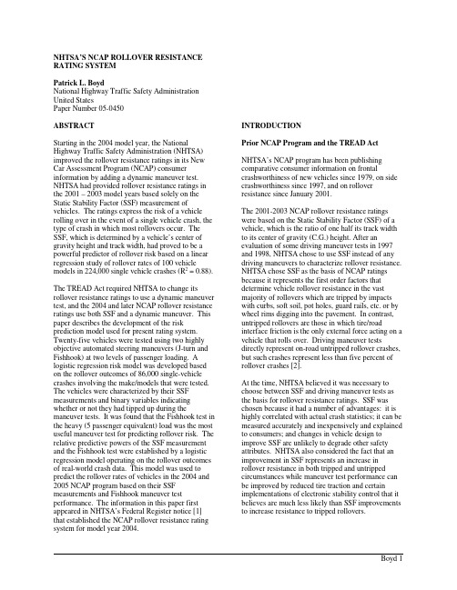
NHTSA’S NCAP ROLLOVER RESISTANCE RATING SYSTEMPatrick L. BoydNational Highway Traffic Safety Administration United StatesPaper Number 05-0450ABSTRACTStarting in the 2004 model year, the National Highway Traffic Safety Administration (NHTSA) improved the rollover resistance ratings in its New Car Assessment Program (NCAP) consumer information by adding a dynamic maneuver test. NHTSA had provided rollover resistance ratings in the 2001 – 2003 model years based solely on the Static Stability Factor (SSF) measurement of vehicles. The ratings express the risk of a vehicle rolling over in the event of a single vehicle crash, the type of crash in which most rollovers occur. The SSF, which is determined by a vehicle’s center of gravity height and track width, had proved to be a powerful predictor of rollover risk based on a linear regression study of rollover rates of 100 vehicle models in 224,000 single vehicle crashes (R2 = 0.88). The TREAD Act required NHTSA to change its rollover resistance ratings to use a dynamic maneuver test, and the 2004 and later NCAP rollover resistance ratings use both SSF and a dynamic maneuver. This paper describes the development of the risk prediction model used for present rating system. Twenty-five vehicles were tested using two highly objective automated steering maneuvers (J-turn and Fishhook) at two levels of passenger loading. A logistic regression risk model was developed based on the rollover outcomes of 86,000 single-vehicle crashes involving the make/models that were tested. The vehicles were characterized by their SSF measurements and binary variables indicating whether or not they had tipped up during the maneuver tests. It was found that the Fishhook test in the heavy (5 passenger equivalent) load was the most useful maneuver test for predicting rollover risk. The relative predictive powers of the SSF measurement and the Fishhook test were established by a logistic regression model operating on the rollover outcomes of real-world crash data. This model was used to predict the rollover rates of vehicles in the 2004 and 2005 NCAP program based on their SSF measurements and Fishhook maneuver test performance. The information in this paper first appeared in NHTSA’s Federal Register notice [1] that established the NCAP rollover resistance rating system for model year 2004. INTRODUCTIONPrior NCAP Program and the TREAD ActNHTSA’s NCAP program has been publishing comparative consumer information on frontal crashworthiness of new vehicles since 1979, on side crashworthiness since 1997, and on rollover resistance since January 2001.The 2001-2003 NCAP rollover resistance ratings were based on the Static Stability Factor (SSF) of a vehicle, which is the ratio of one half its track width to its center of gravity (C.G.) height. After an evaluation of some driving maneuver tests in 1997 and 1998, NHTSA chose to use SSF instead of any driving maneuvers to characterize rollover resistance. NHTSA chose SSF as the basis of NCAP ratings because it represents the first order factors that determine vehicle rollover resistance in the vast majority of rollovers which are tripped by impacts with curbs, soft soil, pot holes, guard rails, etc. or by wheel rims digging into the pavement. In contrast, untripped rollovers are those in which tire/road interface friction is the only external force acting on a vehicle that rolls over. Driving maneuver tests directly represent on-road untripped rollover crashes, but such crashes represent less than five percent of rollover crashes [2].At the time, NHTSA believed it was necessary to choose between SSF and driving maneuver tests as the basis for rollover resistance ratings. SSF was chosen because it had a number of advantages: it is highly correlated with actual crash statistics; it can be measured accurately and inexpensively and explained to consumers; and changes in vehicle design to improve SSF are unlikely to degrade other safety attributes. NHTSA also considered the fact that an improvement in SSF represents an increase in rollover resistance in both tripped and untripped circumstances while maneuver test performance can be improved by reduced tire traction and certain implementations of electronic stability control that it believes are much less likely than SSF improvements to increase resistance to tripped rollovers.Congress directed the agency to enhance the NCAP rollover resistance rating program. Section 12 of the “Transportation Recall, Enhancement, Accountability and Documentation (TREAD) Act of November 2000" directs the Secretary to “develop a dynamic test on rollovers by motor vehicles for a consumer information program; and carry out a program conducting such tests. As the Secretary develops a [rollover] test, the Secretary shall conduct a rulemaking to determine how best to disseminate test results to the public.” The rulemaking was to be carried out by November 1, 2002.Research and Public Comment on Dynamic Rollover TestsOn July 3, 2001, NHTSA published a Request for Comments notice (66 FR 35179) regarding its research plans to assess a number of possible dynamic rollover tests. The notice discussed the possible advantages and disadvantages of various approaches that had been suggested by manufacturers, consumer groups, and NHTSA’s prior research. The driving maneuver tests to be evaluated fit into two broad categories: closed-loop maneuvers in which all test vehicles attempt to follow the same path, and open-loop maneuvers in which all test vehicles are given equivalent steering inputs. The principal theme of the comments was a sharp division of opinion about whether the dynamic rollover test should be a closed loop maneuver test like the ISO 3888 double lane change that emphasizes the handling properties of vehicles or whether it should be an open loop maneuver like a J-Turn or Fishhook that are limit maneuvers in which vulnerable vehicles would actually tip up. Ford recommended a different type of closed loop lane change maneuver in which a path-following robot or a mathematical correction method would be used to evaluate all vehicles on the same set of paths at the same lateral acceleration. It used a measurement of partial wheel unloading without tip-up at 0.7g lateral acceleration as a performance criterion in contrast to the other closed loop maneuver tests that used maximum speed through the maneuver as the performance criterion. Another unique comment was a recommendation from Suzuki to use a sled test developed by Exponent Inc. to simulate tripped rollovers.The subsequent test program [3] (using four SUVs in various load conditions and with and without electronic stability control enabled on two of the SUVs) showed that open-loop maneuver tests using an automated steering controller could be performed with better repeatability of results than the other maneuver tests. The J-Turn maneuver and the Fishhook maneuver (with steering reversal at maximum vehicle roll angle) were found to be the most objective tests of the susceptibility of vehicles to maneuver-induced on-road rollover. Except for the Ford test, the closed loop tests were found not to measure rollover resistance. Instead, the evaluation criterion of maximum maneuver entrance speed measured just prior to entering a double lane change assessed vehicle agility. None of the test vehicles tipped up during runs in which they maintained the prescribed path even when loaded with roof ballast to experimentally reduce their rollover resistance. The speed scores of the test vehicles in the closed loop maneuvers were found to be unrelated to their resistance to tip-up in the open-loop maneuvers that actually caused tip-up. The test vehicle that was clearly the poorest performer in the maneuvers that caused tip-ups achieved the best score (highest speed) in the ISO 3888 and CU short course double lane change, and one vehicle improved its score in the ISO 3888 test when roof ballast was added to reduce its rollover resistance.Due to the non-limit test conditions and the averaging necessary for stable wheel force measurements, the wheel unloading measured in the Ford test appeared to be more quasi-static (as in driving in a circle at a steady speed or placing the vehicle on a centrifuge) than dynamic. Sled tests were not evaluated because NHTSA believed that SSF already provided a good indicator of resistance to tripped rollover. National Academy of Sciences StudyDuring the time NHTSA was evaluating dynamic maneuver tests in response the TREAD Act, the National Academy of Sciences (NAS) was conducting a study of the SSF-based rollover resistance ratings and was directed to make recommendations regarding driving maneuver tests. NHTSA expected the NAS recommendations to have a strong influence on TREAD-mandated changes to NCAP rollover resistance ratings.When NHTSA proposed the prior (SSF only) rollover resistance ratings in June 2000, vehicle manufacturers generally opposed it because they believed that SSF as a measure of rollover resistance is too simple since it does not include the effects of suspension deflections, tire traction and electronic stability control (ESC). In addition, the vehicle manufacturers argued that the influence of vehicle factors on rollover risk is too slight to warrant consumer information ratings for rollover resistance. In the conference report of the FY2001 DOT Appropriations Act, Congress permitted NHTSA tomove forward with its rollover rating program, but directed the agency to fund a National Academy of Sciences (NAS) study on vehicle rollover ratings. The study topics were “whether the static stability factor is a scientifically valid measurement that presents practical, useful information to the public including a comparison of the static stability factor test versus a test with rollover metrics based on dynamic driving conditions that may induce rollover events.” The National Academy’s report was completed and made available at the end of February 2002 [4].The NAS study found that SSF is a scientifically valid measure of rollover resistance for which the underlying physics and real-world crash data are consistent with the conclusion that an increase in SSF reduces the likelihood of rollover. It also found that dynamic tests should complement static measures, such as SSF, rather than replace them in consumer information on rollover resistance. The dynamic tests the NAS recommended would be driving maneuvers used to assess “transient vehicle behavior leading to rollover.”The NAS study also made recommendations concerning the statistical analysis of rollover risk and the representation of ratings. It recommended that NHTSA use logistic regression rather than linear regression for analysis of the relationship between rollover risk and SSF, and it recommended that NHTSA consider a higher-resolution representation of the relationship between rollover risk and SSF than is provided by a five-star rating system. NHTSA published a Federal Register notice on October 7, 2002 (67 FR 62528) that proposed to modify the NCAP rollover resistance ratings to satisfy the requirements of the TREAD Act and to align it with the recommendation of the NAS report. NHTSA chose the J-Turn and Fishhook maneuver (with roll rate feedback) as the dynamic maneuver tests because they were the type of limit maneuver tests that could directly lead to rollover as recommended by the NAS. NHTSA also proposed to use a logistic regression analysis to determine the relationship between vehicle properties and rollover risk, as recommended by the NAS.DYNAMIC MANEUVER TESTS OF 25 VEHICLESThe original NCAP rollover resistance ratings predicted the rate of rollovers per single vehicle crash based on the SSF of vehicles. Stars were used to express rollover risk in rate increments of 10% (i.e., 2 stars for a predicted rollover rate between 30 and 40%, 3 stars for a predicted rollover rate between 20 and 30%, etc.). The relationship between rollover rate and SSF was determined using a linear regression between the logarithm of SSF and the actual rollover rates of 100 vehicle make/models [5]. The rollover rates were determined from 224,000 state crash reports and were corrected for differences between vehicles in demographic and road condition variables reported by the states.The idea for improving the prediction of rollover rate (the risk model) using dynamic maneuver tests was to describe the vehicle by its SSF plus a number of variables resulting from the vehicle’s behavior in the dynamic maneuvers. In that way, the risk model would consider more than just the geometric properties of the vehicle. Four binary variables were anticipated. They would describe whether the vehicle tipped up or did not in the J-turn and in the Fishhook maneuver, each performed with the vehicle in two passenger load configurations. The risk model for predicting rollover rate on the basis of SSF plus dynamic test results would be determined using logistic regression between the rollover outcomes of state crash reports of single vehicle crashes of a number of vehicles and the new set of vehicle attributes (SSF plus dynamic test variables). The expression of rollover risk by stars would continue with the same relationship between the number of stars and the predicted rollover rate.The linear regression, SSF only, risk model used crash data on 100 vehicles, but it was impractical to perform maneuver tests on that many vehicles to develop the present risk model. This section presents an overview of the test maneuvers and the results for the subset of 25 vehicles selected for developing the logistic regression risk model. A more extensive account of the test program is contained in the Phase VI and VII rollover research report [6]. The NHTSA J-Turn and Fishhook (with roll rate feedback) maneuver tests were performed for 25 vehicles representing four vehicle types including passenger cars, vans, pickup trucks and SUVs. NHTSA chose mainly high production vehicles that spanned a wide range of SSF values, using vehicles NHTSA already owned where possible. Except for four 2001 model year vehicles NHTSA purchased new, the vehicle suspensions were rebuilt with new springs and shock absorbers, and other parts as required for all the other vehicles included in the test program.J-Turn ManeuverThe NHTSA J-Turn maneuver represents anavoidance maneuver in which a vehicle is steered away from an obstacle using a single input. The maneuver is similar to the J-Turn used during NHTSA’s 1997-98 rollover research program and is a common maneuver in test programs conducted by vehicle manufacturers and others. Often the J-Turn is conducted with a fixed steering input (handwheel angle) for all test vehicles. In its 1997-98 testing, NHTSA used a fixed handwheel angle of 330 degrees. During the development of the present tests, NHTSA developed an objective method of specifying equivalent handwheel angles for J-Turn tests of various vehicles, taking into account their differences in steering ratio, wheelbase and linear range understeer properties [3]. Under this method, one first measures the handwheel angle that would produce a steady-state lateral acceleration of 0.3 g at 50 mph on a level paved surface for a particular vehicle. In brief, the 0.3 g value was chosen because the steering angle variability associated with this lateral acceleration is quite low and there is no possibility that stability control intervention could confound the test results. Since the magnitude of the handwheel position at 0.3 g is small, it must be multiplied by a scalar to have a high maneuver severity. In the case of the J-Turn, the handwheel angle at 0.3 g was multiplied by eight. When this scalar is multiplied by handwheel angles commonly observed at 0.3 g, the result is approximately 330 degrees. Figure 1 illustrates the J-Turn maneuver in terms of the automated steering inputs commanded by the programmable steering machine. The rate of the handwheel turning is 1000 degrees per second. To begin the maneuver, the vehicle was driven in astraight line at a speed slightly greater than the desired entrance speed. The driver released the throttle, coasted to the target speed, and then triggered the commanded handwheel input. The nominal maneuver entrance speeds used in the J-Turn maneuver ranged from 35 to 60 mph, increased in 5 mph increments until a termination condition was achieved. Termination conditions were simultaneous two inch or greater lift of a vehicle’s inside tires (two-wheel lift) or completion of a test performed at the maximum maneuver entrance speed without two-wheel lift. If two-wheel lift was observed, a downward iteration of vehicle speed was used in 1 mph increments until such lift was no longer detected. Once the lowest speed for which two-wheel lift could be detected was isolated, two additional tests were performed at that speed to monitor two-wheel lift repeatability.Fishhook ManeuverThe Fishhook maneuver uses steering inputs that approximate the steering a driver acting in panic might use in an effort to regain lane position after dropping two wheels off the roadway onto the shoulder. NHTSA has often described it as a road edge recovery maneuver. As pointed out by some commenters, it is performed on a smooth pavement rather than at a road edge drop-off, but its rapid steering input followed by an over-correction is representative of a general loss of control situation. The original version of this test was developed by Toyota, and variations of it were suggested by Nissan and Honda. NHTSA has experimented with several versions since 1997, and the present test includes roll rate feedback in order to time the counter-steer to coincide with the maximum roll angle of each vehicle in response to the first steer.Figure 2 describes the Fishhook maneuver in terms of the automated steering inputs commanded by the programmable steering machine and illustrates the roll rate feedback. The initial steering magnitude and countersteer magnitudes are symmetric, and are calculated by multiplying the handwheel angle that would produce a steady state lateral acceleration of 0.3 g at 50 mph on level pavement by 6.5. When this scalar is multiplied by handwheel angles commonly observed at 0.3 g, the result is approximately 270 degrees. This is equivalent to the 270 degree handwheel angle used in earlier forms of the maneuver but, as in the case of the J-Turn, the procedure above is an objective way of compensating for differences in steering gear ratio, wheelbase and understeer properties between vehicles. The fishhook maneuver dwell times (the time between completion of the initial steering ramp and the initiation of the countersteer) are defined by the roll motion of the vehicle being evaluated, and can vary on a test-to-test basis. This is made possible by having the steeringFigure 1. NHTSA J-turn maneuver description.machine monitor roll rate (roll velocity). If an initial steer is to the left, the steering reversal following completion of the first handwheel ramp occurs when the roll rate of the vehicle first equals or goes below 1.5 degrees per second. If an initial steer is to the right, the steering reversal following completion of the first handwheel ramp occurs when the roll rate of the vehicle first equals or exceeds -1.5 degrees per second. The handwheel rates of the initial steer and countersteer ramps are 720 degrees per second.To begin the maneuver, the vehicle was driven in astraight line at a speed slightly greater than the desired entrance speed. The driver released the throttle, coasted to the target speed, and then triggered the commanded handwheel input described in Figure 2. The nominal maneuver entrance speeds used in the fishhook maneuver ranged from 35 to 50 mph, increased in 5 mph increments until a termination condition was achieved. Termination conditions included simultaneous two inch or greater lift of a vehicle’s inside tires (two-wheel lift) or completion of a test performed at the maximum maneuver entrance speed without two-wheel lift. If two-wheel lift was observed, a downward iteration of vehicle speed was used in 1 mph increments until such lift was no longer detected. Once the lowest speed for which two-wheel lift could be detected was isolated, two additional tests were performed at that speed to check two-wheel lift repeatability.NHTSA observed that during the Fishhook tests, excessive steering caused some vehicles to reach their maximum roll angle response to the initial steering input before it had been fully completed (this is essentially equivalent to a “negative” T1 in Figure 2). Since dwell time duration can have a significant effect on how the Fishhook maneuver’s ability to produce two-wheel lift, excessive steering may stifle the most severe timing of the counter steer for some vehicles. In an attempt to better insure high maneuver severity, a number of vehicles that did not produce two-wheel lift with steering inputs calculated with the 6.5 multiplier were also tested with lesser steering angles by reducing the multiplier to 5.5. This change increased the dwell times observed during the respective maneuvers. Some vehicles tipped up in Fishhook maneuvers conducted at the lower steering angle (5.5 multiplier) but not at the higher steering angle (6.5 multiplier). NHTSA adopted the practice of performing Fishhook maneuvers at both steering angles for NCAP. Loading ConditionsThe vehicles were tested in each maneuver in two load conditions in order to create four levels of stringency in the suite of maneuver tests. The light load was the test driver plus instrumentation in the front passenger seat, which represented two occupants. A heavier load was used to create a higher level of stringency for each test. In our NPRM, NHTSA announced that the heavy load would include 175 lb anthropomorphic forms (water dummies) in all rear seat positions. During the test of the 25 vehicles, it became obvious that heavy load tests were being run at very unequal load conditions especially between vans and other vehicles (two water dummies in some vehicles but six water dummies in others). While very heavy passenger loads can certainly reduce rollover resistance and potentially cause special problems, crashes at those loads are too few to greatly influence the overall rollover rate of vehicles. Over 94% of van rollovers in our 293,000 crash database occurred with five or fewer occupants, and over 99% of rollovers of other vehicles occurred with five or fewer occupants. The average passenger load of vehicles in our crash database was less than two: 1.81 for vans; 1.54 for SUVs; 1.48 for cars; and 1.35 for pickup trucks. In order to use the maneuver tests to predict real-world rollover rates, it seemed inappropriate to test theFigure 2. NHTSA Fishhook maneuver description.vehicles under widely differing loads that did not correspond to the real-world crash statistics. Therefore, the tests used to develop a statistical model of rollover risk were changed to a uniform heavy load condition of three water dummies (representing a 5-occupant loading) for all vehicles capable of carrying at least five occupants. Some vehicles were loaded with only two water dummies because they were designed for four occupants. For pickup trucks, water dummies were loaded in the bed at approximately the same height as a passenger in the front seat.Test ResultsThe test results in Table 1 (presented on the next page) reflect the performance as described for a heavy load condition representing five occupants except for the Ford Explorer 2DR, the Chevrolet Tracker and Metro that were designed for only four occupants, and the Honda CRV, Honda Civic and Chevrolet Cavalier that could not be loaded to the 5-occupant level without exceeding a gross axle weight rating because of the additional weight of the outriggers.Each test vehicle in Table 1 represented a generation of vehicles whose model year range is given. Twenty-four of the vehicles were taken from 100 vehicle groups whose 1994-98 crash statistics in six states were the basis of the present SSF based rollover resistance ratings. The nominal SSFs used to describe the vehicle groups in the prior statistical studies are given. While there were some variations between the SSFs of the individual test vehicles and the nominal vehicle group SSF values, the nominal SSFs were retained for the present statistical analyses because they represent vehicles produced over a wide range of years in many cases and provide a simple comparison between the risk model presented in this notice and that discussed in the previous notices. The X’s under the various test maneuver names indicate which vehicles tipped up during the tests. Eleven of the twenty-five vehicles tipped up in the Fishhook maneuver conducted in the heavy condition. The heavy condition represented a five-occupant load for all vehicles except the six mentioned above that were limited to a four-occupant load by the vehicle seating positions and GVWR. All eleven were among the sixteen test vehicles with SSFs less than 1.20. None of the vehicles with higher SSFs tipped up in any test maneuver. The Fishhook test under the heavy load clearly had the greatest potential to cause tip-up. The groups of vehicles that tipped up in other tests were subsets of the larger group of eleven that tipped up in the Fishhook Heavy test. There were seven vehicles in the group that tipped up in the J-Turn Heavy test, six of which also tipped up in the Fishhook Light test. The J-Turn Light test had the least potential to tip up vehicles. Only three vehicles tipped up, all of which had tipped up in every other test.ROLLOVER RISK MODELIn its study of NHTSA’s rating system for rollover resistance [4], the National Academy of Sciences (NAS) recommended that NHTSA use logistic regression rather than linear regression for analysis of the relationship between rollover risk and SSF. Logistic regression has the advantage that it operates on every crash data point directly rather than requiring that the crash data be aggregated by vehicle and state into a smaller number of data points. For example, NHTSA now has state data reports of about 293,000 single-vehicle crashes of the hundred vehicle make/models (together with their corporate cousins) whose single-vehicle crashes NHTSA have been tracking in six states. The logistic regression analysis of this data would have a sample size of 293,000, producing a narrow confidence interval on the repeatability of the relationship between SSF and rollover rate. In contrast, the linear regression analysis operates on the rollover rate of the hundred vehicle make/models in each of the six states. It produces a maximum sample size of only 600 (100 vehicles times six states) minus the number of samples for which fewer than 25 crashes were available for determining the rollover rate (a data quality control practice). Confidence limits computed for a data sample size of 600 will be much greater than those based on a sample size of 293,000. On average, each sample in the linear regression analysis was computed from over 400 crash report samples. However, ordinary techniques to compute the confidence intervals of linear regression results do not take into account the actual sample size represented by aggregated data. The statistical model created to combine SSF and dynamic test information in the prediction of rollover risk was computed by means of logistic regression as recommended by the NAS. Logistic regression is well suited to the correlation with crash data of vehicle properties that include both continuous variables like SSF and binary variables like tip-up or no tip-up in maneuver tests.NHTSA had previously considered logistic regression during the development of the SSF based rating system [4], but found that it consistently under-predicted the actual rollover rate at the low end of the。
电工英语词汇

电路的基本概念及定律电源source [sɔ:s]电压源voltage source电流源current source理想电压源ideal voltage source理想电流源ideal current source伏安特性volt-ampere characteristic电动势electromotive force电压voltage['vəultidʒ]电流current['kʌrənt]电位potential[pəu'tenʃəl]电位差potential difference欧姆Ohm伏特Volt安培Ampere瓦特Watt焦耳Joule电路circuit电路元件circuit element电阻resistance电阻器resistor电感inductance电感器inductor电容capacitance电容器capacitor电路模型circuit model参考方向reference direction 参考电位reference potential欧姆定律Ohm’s law基尔霍夫定律Kirchhoff’s law基尔霍夫电压定律Kirchhoff’svoltage law(KVL)基尔霍夫电流定律Kirchhoff’scurrent law(KCL)结点node支路branch回路loop网孔mesh支路电流法branch current analysis网孔电流法mesh current analysis 结点电位法node voltage analysis 电源变换source transformations叠加原理superposition theorem网络network无源二端网络passive two-terminal network有源二端网络active two-terminal network戴维宁定理Thevenin’s theorem诺顿定理Norton’s theorem开路(断路)open circuit短路short circuit开路电压open-circuit voltage短路电流short-circuit current交流电路直流电路direct current circuit (dc)交流电路alternating current circuit (ac)正弦交流电路sinusoidal a-c circuit平均值average value有效值effective value均方根值root-mean-squire value (rms)瞬时值instantaneous value电抗reactance感抗inductive reactance容抗capacitive reactance法拉Farad亨利Henry阻抗impedance复数阻抗complex impedance相位phase初相位initial phase相位差phase difference相位领先phase lead相位落后phase lag倒相,反相phase inversion频率frequency角频率angular frequency 赫兹Hertz相量phasor相量图phasor diagram有功功率active power无功功率reactive power视在功率apparent power功率因数power factor功率因数补偿power-factor compensation串联谐振series resonance并联谐振parallel resonance谐振频率resonance frequency频率特性frequency characteristic 幅频特性amplitude-frequencyresponsecharacteristic相频特性phase-frequencyresponsecharacteristic截止频率cutoff frequency品质因数quality factor通频带pass-band带宽bandwidth (BW)滤波器filter一阶滤波器first-order filter二阶滤波器second-order filter低通滤波器low-pass filter高通滤波器high-pass filter带通滤波器band-pass filter带阻滤波器band-stop filter转移函数transfer function波特图Bode diagram傅立叶级数Fourier series三相电路三相电路three-phase circuit三相电源three-phase source对称三相电源symmetricalthree-phasesource对称三相负载symmetrical three-phase load相电压phase voltage相电流phase current线电压line voltage线电流line current三相三线制three-phase three-wire system三相四线制three-phase four-wire system三相功率three-phase power星形连接star connection(Y-connection)三角形连接triangularconnection( -connection ,deltaconnection)中线neutral line 电路的暂态过程分析暂态transient state稳态steady state暂态过程,暂态响应transient response换路定理low of switch一阶电路first-order circuit三要素法three-factor method时间常数time constant积分电路integrating circuit微分电路differentiating circuit磁路与变压器磁场magnetic field磁通flux磁路magnetic circuit磁感应强度flux density磁通势magnetomotive force磁阻reluctance电动机直流电动机dc motor交流电动机ac motor异步电动机asynchronous motor同步电动机synchronous motor三相异步电动机three-phaseasynchronousmotor单相异步电动机single-phaseasynchronousmotor旋转磁场rotating magnetic field 定子stator转子rotor转差率slip起动电流starting current起动转矩starting torque额定电压rated voltage额定电流rated current额定功率rated power机械特性mechanical characteristic继电器-接触器控制按钮button熔断器fuse开关switch行程开关travel switch继电器relay接触器contactor常开(动合)触点normally open contact常闭(动断)触点normally closed contact时间继电器time relay热继电器thermal overload relay中间继电器intermediate relay可编程控制器(PLC)可编程控制器programmable logic controller语句表statement list梯形图ladder diagram半导体器件本征半导体intrinsic semiconductor掺杂半导体doped semiconductor P型半导体P-type semiconductor N型半导体N--type semiconductor自由电子free electron空穴hole载流子carriersPN结PN junction扩散diffusion漂移drift二极管diode硅二极管silicon diode锗二极管germanium diode阳极anode阴极cathode发光二极管light-emitting diode (LED)光电二极管photodiode稳压二极管Zener diode晶体管(三极管)transistor PNP型晶体管PNP transistor NPN型晶体管NPN transistor发射极emitter集电极collector基极base电流放大系数current amplification coefficient场效应管field-effect transistor (FET)P沟道p-channelN沟道n-channel结型场效应管junction FET (JFET)金属氧化物半导体metal-oxide semiconductor (MOS)耗尽型MOS场效应管depletion mode MOSFET(D-MOSFET)增强型MOS场效应管enhancement mode MOSFET (E-MOSFET)源极source栅极grid漏极drain跨导transconductance夹断电压pinch-off voltage热敏电阻thermistor开路open短路shorted基本放大器放大器amplifier正向偏置forward bias 反向偏置backward bias静态工作点quiescent point (Q-point)等效电路equivalent circuit电压放大倍数voltage gain总的电压放大倍数overall voltage gain饱和saturation截止cut-off放大区amplifier region饱和区saturation region截止区cut-off region失真distortion饱和失真saturation distortion截止失真cut-off distortion零点漂移zero drift正反馈positive feedback负反馈negative feedback串联负反馈series negative feedback并联负反馈parallel negative feedback共射极放大器common-emitter amplifier射极跟随器emitter-follower共源极放大器common-source amplifier共漏极放大器common-drain amplifier多级放大器multistage amplifier 阻容耦合放大器resistance-capacitance coupled amplifier直接耦合放大器direct- coupled amplifier输入电阻input resistance输出电阻output resistance负载电阻load resistance动态电阻dynamic resistance负载电流load current旁路电容bypass capacitor耦合电容coupled capacitor直流通路direct current path交流通路alternating current path 直流分量direct current component交流分量alternating current component变阻器(电位器)rheostat电阻(器)resistor电阻(值)resistance电容(器)capacitor电容(量)capacitance电感(器,线圈)inductor电感(量),感应系数inductance 正弦电压sinusoidal voltage集成运算放大器及应用差动放大器differential amplifier 运算放大器operational amplifier(op-amp)失调电压offset voltage失调电流offset current共模信号common-mode signal差模信号different-mode signal共模抑制比common-mode rejection ratio (CMRR)积分电路integrator(circuit)微分电路differentiator(circuit)有源滤波器active filter低通滤波器low-pass filter高通滤波器high-pass filter带通滤波器band-pass filter带阻滤波器band-stop filter波特沃斯滤波器Butterworth filter切比雪夫滤波器Chebyshev filter 贝塞尔滤波器Bessel filter截止频率cut-off frequency上限截止频率upper cut-off frequency下限截止频率lower cut-off frequency中心频率center frequency带宽Bandwidth开环增益open-loop gain闭环增益closed-loop gain共模增益common-mode gain输入阻抗input impedance电压跟随器voltage-follower电压源voltage source电流源current source单位增益带宽unity-gain bandwidth频率响应frequency response频响特性(曲线)response characteristic波特图the Bode plot稳定性stability补偿compensation比较器comparator迟滞比较器hysteresis comparator 阶跃输入电压step input voltage仪表放大器instrumentation amplifier隔离放大器isolation amplifier对数放大器log amplifier反对数放大器antilog amplifier反馈通道feedback path反向漏电流reverse leakage current相位phase相移phase shift锁相环phase-locked loop(PLL)锁相环相位监测器PLL phase detector和频sum frequency 差频difference frequency波形发生电路振荡器oscillatorRC振荡器 RC oscillatorLC振荡器 LC oscillator正弦波振荡器sinusoidal oscillator三角波发生器triangular wave generator方波发生器square wave generator 幅度magnitude电平level饱和输出电平(电压)saturated output level功率放大器功率放大器power amplifier交越失真cross-over distortion甲类功率放大器class A power amplifier乙类推挽功率放大器class B push-pull power amplifierOTL功率放大器output transformerless power amplifier OCL功率放大器output capacitorless power amplifier直流稳压电源半波整流full-wave rectifier全波整流half-wave rectifier电感滤波器inductor filter电容滤波器capacitor filter串联型稳压电源series (voltage) regulator开关型稳压电源switching (voltage) regulator集成稳压器IC (voltage) regulator 晶闸管及可控整流电路晶闸管thyristor单结晶体管unijunction transistor (UJT)可控整流controlled rectifier可控硅silicon-controlled rectifier 峰点peak point谷点valley point控制角controlling angle导通角turn-on angle门电路与逻辑代数二进制binary二进制数binary number十进制decimal十六进制hexadecimal二-十进制binary coded decimal (BCD)门电路gate三态门tri-state gate与门AND gate或门OR gate非门NOT gate与非门NAND gate 或非门NOR gate异或门exclusive-OR gate反相器inverter布尔代数Boolean algebra真值表truth table卡诺图the Karnaugh map逻辑函数logic function逻辑表达式logic expression组合逻辑电路组合逻辑电路combination logic circuit译码器decoder编码器coder比较器comparator半加器half-adder全加器full-adder七段显示器seven-segment display时序逻辑电路时序逻辑电路sequential logic circuitR-S 触发器R-S flip-flopD触发器 D flip-flopJ-K触发器J-K flip-flop主从型触发器 master-slave flip-flop置位set复位reset直接置位端direct-set terminal直接复位端direct-reset terminal寄存器register移位寄存器shift register双向移位寄存器bidirectional shift register计数器counter同步计数器synchronous counter 异步计数器asynchronous counter 加法计数器adding counter减法计数器subtracting counter 定时器timer清除(清0)clear载入load时钟脉冲clock pulse触发脉冲trigger pulse上升沿positive edge下降沿negative edge时序图timing diagram波形图waveform脉冲波形的产生与整形单稳态触发器monostable flip-flop双稳态触发器bistable flip-flop无稳态振荡器astable oscillator晶体crystal555定时器555 timer模拟信号与数字信号的相互转换模拟信号analog signal数字信号digital signal AD转换器analog -digital converter (ADC)DA转换器digital-analog converter (DAC)半导体存储器只读存储器read-only memory (ROM)随机存取存储器random-access memory(RAM)可编程ROM programmable ROM (PROM)。
超高镍正极材料主要研究内容

超高镍正极材料主要研究内容英文版With the increasing demand for high-energy-density batteries, researchers have been focusing on developing advanced electrode materials for lithium-ion batteries. Among these materials, high-nickel content cathodes have attracted significant attention due to their high specific capacity and energy density.The main research focus on high-nickel cathode materials includes optimizing the nickel content, improving the structural stability, enhancing the rate performance, and increasing the cycling stability. Researchers are also exploring different synthesis methods, such as solid-state reactions, sol-gel methods, and hydrothermal processes, to prepare high-nickel cathode materials with improved electrochemical performance.In addition, researchers are investigating the effect of various dopants, coatings, and surface modifications on the electrochemical performance of high-nickel cathode materials. These strategies aim to mitigate the capacity fading, voltage decay, and thermal instability commonly observed in high-nickel cathodes.Overall, the main research content on high-nickel cathode materials includes nickel content optimization, structural stability improvement, rate performance enhancement, cycling stability increase, synthesis method exploration, dopant effect investigation, and surface modification study. By addressing these research areas, scientists aim to develop high-performance high-nickel cathode materials for next-generation lithium-ion batteries.完整中文翻译随着对高能量密度电池的需求不断增加,研究人员一直致力于开发用于锂离子电池的先进电极材料。
电力系统静态电压稳定性的研究汇总

山东大学硕士学位论文电力系统静态电压稳定性的研究姓名:于永进申请学位级别:硕士专业:电力系统及其自动化指导教师:栾兆文20050510山东大学硕士学位论文摘要近年来,电力系统电压稳定性的研究受到普遍关注。
本文以电压静态稳定性为研究方向,综述了静态电压稳定性常见的计算方法,着重致力于静态电压稳定判据的推导以及静态电压稳定指标的求取,并就其他一些相关内容进行了较为深入的讨论。
本文首先对利用PV曲线的aP/≤V判据做简单回顾,讨论负荷特性对电压稳定性的影响。
在广义雅可比矩阵的基础上,推导出考虑负荷特性的静态电压稳定条件,然后结合鼻型曲线的特点,推导出考虑负荷特性的静态电压稳定实用判掘,并指出:系统在鼻型曲线上半支运行时的静态电压稳定性主要取决于网络的电压一功率传输特性,而系统在鼻型曲线下半支运行时的静态电压稳定性主要取决于负荷的静态电压特性。
电力系统的电压失稳、电压崩溃、及负荷失稳是电压稳定问题中最基本的重要概念,它们既相互联系又有本质区别。
正确和客观地认识它们之间的关系,对深入研究电压稳定问题的机理具有重要意义。
负荷稳定性是电力系统电压稳定性的最主要和最关键的方面。
本文综述和比较了静态电压稳定性指标,根据戴维南等值将整个系统等值为一简单的两节点系统,在此基础上进行电压稳定性分析,推出一种根据定义的节点电压稳定性的指标VSI能快速估计节点电压稳定和求取临界负荷因子k‘的方法,并将该方法扩展到考虑负荷特性和无功限制的情况。
算例分析表明,该方法是一种简单、快速、有效的方法。
最后,本文从系统特性方面探讨了影响电压稳定性的因素,这不仅对静态指标的构造有一定指导作用,更为主要的是为采取措施以最大限度地提高系统稳定性提供理论基础。
关键词:电压稳定:实用判据;电压崩溃;静态电压稳定指标;负荷因子;无功限制Ill山东大学硕士学位论文Abstract:Duringrecentyearsthestudyonvoltagestabilityhasalreadyreceivedwidespreadattentionofmanyresearches.Concentratingonthestaticvoltagestability,thispapersummarizesthecommoncalculationmethodsofstaticvoltagesstabilityandpaysmoreattentiononthestaticvoitagestabilitycriterionandthestaticvoltagestabilityindex.Manyothermattersrelatedtostaticvoltagestabilityarealsodiscussed.Firstly,thepaperreviews%矿。
- 1、下载文档前请自行甄别文档内容的完整性,平台不提供额外的编辑、内容补充、找答案等附加服务。
- 2、"仅部分预览"的文档,不可在线预览部分如存在完整性等问题,可反馈申请退款(可完整预览的文档不适用该条件!)。
- 3、如文档侵犯您的权益,请联系客服反馈,我们会尽快为您处理(人工客服工作时间:9:00-18:30)。
Static Voltage Stability Enhancement Using FACTSControllerIsaiah G. Adebayo1 , Adisa A. Jimoh 2 , Adedayo A. Yusuff 3 , C. Subramani 41,2,3Department of Electrical Engineering, Tshwane University of Technology, Pretoria, South Africa.4Department of Electrical and Electronics Engineering, SRM University, Kanchipuram, India1 isaiahadebayo@, 2Jimohaa@tut.ac.za, 3Yusuffaa@tut.ac.za, 4csmsrm@Abstract— The modern day power system is faced with challenges of voltage instability and has become a great concern to the power system industries. In this work, we proposed a technique of the Network structural Characteristics Participation Factor (NSCPF) to identify the most critical node where reactive power compensator can be placed for voltage stability enhancement. The approach is based on the use of eigenvalue decomposition technique on the submatrix of the partitioned bus admittance matrix. Conventional power flow based approach of voltage stability index (L-Index) and the modal analysis methods are used as benchmarks to the proposed approach to determine its effectiveness. The STATCOM FACTS controller is in turn installed at the critical bus as identified by both techniques. Simulation results obtained show that, the suggested approach saves time and is more advantageous in identifying the suitable bus for the placement of STATCOM.Keywords— Power flow, Power electronics, Voltage stability indices, Network Structural characteristics, Modal AnalysisI.INTRODUCTIONPower system voltage stability is a complex matter that has been challenging the power system utilities in the past two decades [1],[2]. The continuous increase in power demand and more interconnections with limited transmission expansion has been a demanding task to operate the power system in an efficient way [3]. The consequence of the occurrence of voltage instability in power systems may be very catastrophic as this could lead to voltage collapse [4]. This incident is characterized by a slow variation in the system operating point, as a result of increase in loads, in such a manner that voltage magnitudes gradually decrease until a sharp, accelerated change occurs [5].A number of major blackouts throughout the world have been directly related with this phenomenon, for example, the blackout experienced in 2003 in North America, and later in Europe, New Zealand, France, Iran, Belgium, Japan and so on [6]. Thus, it has become a major threat and concern to the power system operators and has been considered as an active area of research in the recent year. Over the years, considerable attempts have been made by several researchers to curb the occurrence of voltage collapse in power systems. The use of PV and QV curves have gained much attention since the incident of voltage collapse in Tokyo and are well documented in the literature [7],[8]. These techniques are computationally demanding and are time consuming, especially for large and complex networks. Other voltage instability and voltage collapse prediction techniques reported in the literature [9] include continuation power flow (CPF) method [10], modal analysis [11], the minimum singular value of the power flow Jacobian [12], voltage instability proximity indicator [13].The use of these methods, however, is time consuming and laborious, particularly for a large power system network as it involves performing a power flow solution before a collapse point is detected. Most recently, considerable stability indices have been introduced and developed in the literatures to assess the condition of system voltage stability. These indices include, among others voltage stability index (L-index), voltage collapse proximity index (VCPI), Line stability index, Line stability factor (LPQ) and Fast Voltage stability index (FVSI) [1], [14]-[16]. Although, the use of these indices has helped system operators a lot, especially to determine the bus that is susceptible to collapse. However, the process is always too tedious and time consuming as it requires performing a multiple power flow before the point is detected. Thus, there is a need for a reliable and fast tool for voltage collapse point detection in power system.Although a considerable effort has been made by the author of [17] in detecting nodes suitable for optimal location of reactive power compensators for voltage stability enhancement, however, the best nodes identified by the authors for the placement of compensators may not be the most critical, as their work did not capture the bus which participate (contribute) most to the smallest eigenvalue (critical mode) identified. FACTS devices are mostly used to provide power flow and voltage control in many utilities. The use of FACTS controller devices such as UPFC, STATCOM, SVC, GUPFC, TCSC, IPFC among others, for voltage control is well documented in the open literatures [11],[18],[19].In this paper, we suggest an approach based on the network topological characteristics of power system which makes use of the critical mode and the associated eigenvectors978-1-5090-3751-3/16/$31.00 ©2016 IEEEto compute the weak nodes where reactive power compensator can be placed. Comparative analysis of this approach is done with the existing power flow based L-index. All the techniques presented are tested on the IEEE 5 bus and the practical 26-bus test systems. The STATCOM FACTS deviceis used as a reactive compensator device for voltage stabilityenhancement in this paper. The remaining of this paper isorganized as follows: Section II gives the mathematical formulation of the suggested approach of the NSCPF and a brief note on the conventional power flow based L-Index technique, while a brief description of the STATCOM used is presented in Section III. Section IV present result and discussion of the work and the conclusion of the work is presented in Section V. II. PROBLEM FORMULATIONSMathematical formulations of NSCTPF start from thebasic law of circuit theory. It is derived by partitioning the Y-admittance matrix into four regions as shown in (1)»¼º«¬ª»¼º«¬ª=»¼º«¬ªL G LL LG GL GG L G V V Y Y Y Y I I (1) »¼º«¬ª=LL LG GL GG Y Y Y Y Y (2)If we further expand (1) and manipulate the resulting algebraic equations, we have;»¼º«¬ª»¼º«¬ª=»¼º«¬ªL G LL LG GL GG L G V I D W H Z I V (3) where[][]1−=GG GG Y Z[][][]GL GG GL Y Y H 1−−= [][][]1−=GG LG LG Y Y W[][][][][]GL GG LG LL LL Y Z Y Y D −=The eigenvalue decomposition of matrix LL D is given by *1*i ini i LL f f F F D ξξ¦===(4)whereF is an orthonormal matrix with eigenvectors i f and ξis a diagonal matrix with eigenvalues i ξ.Expanding (3) also results in:[][][][]{}G LG L LLL I W I D V −=−1(5)Substitution of (21) in (22)[][][][]{}G LG L n i i i i L I W I v V −¼º«¬ª=¦=1*ξν (6)From (5) and (6), it can be seen that large values of iξdepicts small changes in the load voltage. However, as thesystem is stressed, the value of i ξ becomes smaller and theload voltage becomes weaker. If the magnitude of i ξis equal to zero, the corresponding load voltage collapses. The weak load bus is surrounded by lines with high impedances. The extent of whether the reactive elements are not enough or sufficient in power system is solely depends on the participation between network buses observable from the eigenvectors of the matrix F. In some occasions, the criticalbus, which is associated to the smallest eigenvalue may not be a more critical load bus.Thus, this present work digs deep to further explore theconcept of structural based participation factor to determinethe most critical load bus, which contributes most to thesmallest eigenvalue as identified using (4) for voltage stabilityenhancement. We termed this Network Structural Characteristics Theory-Participation Factor (NSCTPF) in this work. This is done by identifying the elements contributingmost in these modes. The bus participation factor measuring the contribution of the th i bus to the thj mode is the product of right and left eigenvectors defined in (7) and it is given asji ij ij f f NSCTPF =(7)It follows that, the bus, which has large participation factorscorresponds to the most critical system buses which are liable to voltage collapse.L-index proposed by [20] and the modal analysis of the reduced Jacobian matrix [11] are used in this work as benchmarks to test the effectiveness of the proposed approach of NSCTPF. With these techniques, the suitable locations for the STATCOM FACTS device are determined. Details of the mathematical formulations of the L-Index and the modal analysis techniques are reported in [20] and [11] respectively. The L index varies in a range between 0 (no load) and 1 (voltage collapse). The maximum of these indices gives the proximity of the system voltage collapse. For the modal analysis, the bus with the highest value of the Modal Analysis Participation Factor (MAPF) is usually considered the critical bus.II STATCOM FACTS CONTROLLERSTATCOM is a shunt-connected device, which regulates the voltage at the connected bus to the reference value by controlling the voltage and angle of internal voltage source. The resulting STATCOM can inject or absorb reactive power to or from the bus to which it is connected and thus control the bus voltage magnitude. The STATCOM has the capacity to either inject or absorb the reactive power of the system, depending on the voltage magnitude to which it is connected into. When system voltage is low, the STATCOM injectsreactive power (STATCOM capacitive). When system voltage is high, it absorbs reactive power (STATCOM inductive). There are two major models of STATCOM reported in the literatures. These models have been well tested in power systems. Namely, the Current Injection Model (CIM) and the Power Injection Model (PIM) [21],[22]. In the CIM, STATCOM has a current source connected in shunt to the bus for voltage magnitude control. The PIM model of the STATCOM is a shunt voltage source behind an equivalent reactance or impedance, which is also referred to as a voltage source model (VSM). This steady state power injection model of STATCOM has proved to be reliable when incorporated in power systems. Details formulation of the power injection model is well reported in [23].IV SIMULATION RESULTS AND DISCUSSIONThe effectiveness of all the approaches presented is tested on both IEEE 5 bus and the practical 26-bus power systems. The IEEE 5 bus test system consists of two generators, three load buses seven transmission lines . On the other hand, the 26 bus practical power system consists of six generator buses, twenty load buses and forty six transmission lines. All the data used for the 26-bus system is taken from [24]. In this paper, the generator and load buses are arranged sequentially. Load buses 24, 25, 21, 19 and 17 of the 26 bus power system are selected at random for voltage stability analysis. MATLAB 2014b are used as simulation tools in this work. Results and discussions of the IEEE 5 bus and the 26 bus test systems, respectively are presented in this section.A.The IEEE 5 bus test systemFor the proposed NSCPF, first, we applied the eigenvalues decomposition on the matrix of (4) to identify the critical mode of the system. This matrix shows the electrical interconnection between the load buses in the power system network. It is based on the admittance matrix of the system. The associated network structural based eigenvectors are then used to compute the values of the Network Structural Characteristics Participation Factor (NSCPF) of each load bus. The results of the eigenvalues of each load bus, with the corresponding mode, NSCPF and the total computational time obtained for the IEEE 5 test systems are as presented in Table I.Load bus 4 which corresponds to the mode 2 of the IEEE 5 bus system has the highest value of the NSCPF (0.4468) , thus it is considered as the weak bus of the network where reactive power compensator may be placed for voltage stability enhancement.The traditional power flow based results of the modal analysis and the L-index techniques for the IEEE 5 bus system are as shown in Table II and III respectively. It could be seen that the results of the modal analysis obtained are in agreement with that obtained for the proposed NSCPF. This is as shown in Table II. Bus 4 has the maximum value of MAPF (0.3749) and corresponds to mode 2 of the system. Thus, this bus is considered as the weakest of all the load buses of the IEEE 5 bus system. Worth-noting is the similarity between the proposed NSCPF and the MAPF. The difference between the two approaches, however, is obvious. The formal depends on the network structural interconnections of buses in power system and are non-iterative in nature. They are captured by the admittance matrix of the system.On the other hand, the MAPF is power flow based and are iterative. It depends solely on the active and reactive power loads of the system and the Jacobian matrices. With the L-Index approach, bus 5 is found to have the least allowable loads of 260MVar and maximum values of L-Index (1.0102), with the least voltage magnitude (0.5321). Thus, based on this approach, bus 5 is identified as the bus suitable for the injection of reactive power. It must be stated, however, that it only takes just a single computational step to attain a solution with the proposed method of NSCPF (1.207473), whereas, it takes longer period of time for the power flow based approaches, with the exception of the modal analysis.B.The 26 – bus practical power systemSimilar procedures as presented for the case of IEEE 5 bus system are also followed here. The results of the NSCPF-Eigenvalues for each load bus of the 26-bus system are as presented in Figure 1. Also presented in Table IV are the results of simulations obtained for the conventional power flow based L-Index approach and the proposed NSCPF. The results of voltage magnitude obtained with the computational time at each reactive power load variation for the selected load buses 17, 19, 21, 24 and 25 are also shown in Table IV. The results of the MAPF of each selected load buses of the 26-bus system are also represented in Table V.Fig. 1: NSCPF Eigenvalues of 26-bus systemWith the suggested technique based on the network topological structure of power systems, of the five weak load buses 17,19,21,24 and 25 selected, bus 24 is found to have the maximum value of NSCPF (0.4238) and also correspond to mode 10 of the 26 – bus practical power system as shown in Table IV and Figure 1 respectively. Similar results are also obtained for the conventional power flow based approaches, except that bus 25 is ranked as the weakest bus of the 26-bus power system with the modal analysis method.C. Voltage Stability Enhancement with STATCOM FACTSDevicePresented in this section are the results obtained when the STATCOM is placed on the weak buses identified by the approaches considered for both the IEEE 5 bus and the 26 bus power systems. STATCOM is placed at the load buses randomly selected for the 26 bus power system and at the three load buses of the IEEE 5 bus system. The result of the voltage magnitude improvement obtained for the IEEE 5 bus and the 26 bus power systems when STATCOM is placed at buses 3,4 and 5 of the IEEE 5 bus system and load buses 17, 19 , 21, 24 and 25 of the 26 bus systems are as presented in the figures 2 to 4 and figures 5 to 9 respectively.TABLE IResults of the proposed NSCPF for the IEEE 5 bus test systemTABLE IIResults of the MAPF obtained for the IEEE 5 bus systemTABLE IIIResults of the L-Index obtained for the IEEE 5 bus systemTable IVResults of the L-Index and NSCTPFTABLE VResults of the MAPF for the 26-bus power systemsWhen STATCOM is placed on load buses 3,4 and 5 of the IEEE 5 bus system, one after the other, there is a considerable improvement in the voltage profile of the system.However, it could be observed that the voltage profile Improvement of the load buses is more obvious when STATCOM is located at bus 4, being the weakest load bus identified by both the proposed NSCPF and the modal analysis of the reduced Jacobian techniques. This is as shown in Figure 6. For instance, the basecase voltage magnitude of bus 4 is 0.9664p.u. With the injection of reactive power through the placement of STATCOM FACTS device, the voltage profile increases to 1.0405 p.u. Similarly, for the 26-bus power system, with the placement of STATCOM on load bus 24, the voltage magnitude of the entire buses also increases.RankBusNo BasecaseVoltagemag(p.u)NSCPF-EigenvaluesModes NSCPF ComputationalTime (secs)2nd 3 0.9652 3.6483 1 0.41901st 4 0.9664 8.9915 2 0.4468 1.207473 3rd 5 0.9656 72.4611 3 0.1342Rank BusNo Eigenvalues Mode MAPF ComputationalTime(secs)2nd 3 73.5592 1 0.34201st 4 7.2398 2 0.3749 2.672109 3rd 5 13.5385 3 0.2831Ranking order BusNoQmax(MVar)L-IndexVoltageMag. (p.u)ComputationalTime (secs)3rd 3 350 1.0003 0.5573 10.208304 2nd 4 345 1.0068 0.5382 6.903298 1st 5 260 1.0102 0.5321 5.609871Bus No Qmax VoltageMag(p.u)L-index Computationaltime (secs)ProposedNSCTPFComputationaltime (secs)21430 0.5666 0.8661 13.340921 0.170624 237 0.5574 0.9223 8.023498 0.423825 238 0.5616 0.8940 10.983421 0.0171 4.908761 19550 0.5858 0.8461 23.023145 0.109117520 0.5796 0.7801 20.210987 0.0631Rank BusNo Eigenvalues MAPF ComputationalTime (secs)5th 17 5.0278 0.00173rd 19 45.0131 0.1065 5.672109 4th21 39.5662 0.06302nd24 25.9740 0.18571st25 28.3753 0.2554For example, there is a drastic voltage drop (basecase) at bus 24 as shown in Figure 8 the basecase voltage magnitude of bus 24. However, with the incorporation of STATCOM at bus 24, the voltage magnitude of targeted bus increases rapidly and so also are the voltage magnitude of other load buses. Similar trend of voltage profile improvement can be observed when STATCOM is placed at buses 17, 19, 21 and 25 as shown in Figures 5, 6, 7 and 9 respectively.Fig. 2. STATCOM at bus 3Fig.3. STATCOM at bus 4 Fig. 4. STATCOM at bus 5 Fig. 5. STATCOM at bus 17Fig. 6. STATCOM at bus 19Fig. 7. STATCOM at bus 21V CONCLUSIONA new approach based on the network structural properties of power system is presented in this paper. The effectiveness of this approach and the conventional power flow based techniques presented is tested on both the IEEE 5 bus and the 26-bus practical power systems. The main aim is to ensure voltage stability enhancement through the incorporation of the STATCOM FACTS device. The weakest bus of the IEEE 5 bus and the 26-bus practical power systems are first identified through the techniques presented. This bus is taken as the best location for the reactive power compensator. The result obtained shows that, bus, suitable for the placement of STATCOM is better identified through the proposed NSCPF compared with the conventional approaches. The suggested technique saves time and requires less computational effort before the weakest bus is identified. This is a great advantage when considering the present Smart Grid system and will also go a long way to aid the power utilities in the operation and planning of the power system.ACKNOWLEDGMENTThe authors acknowledge the financial support received from the Tshwane University of Technology and Rand Water, Pretoria, South AfricaFig. 8. STATCOM at bus 24Fig. 9. STATCOM at bus 25REFERENCES[1] V. Balamourougan, T.S. Sidhu & M.S. Sachdev. “Technique for onlinePrediction of voltage collapse”, IEEE Proc. Gener. Transm. Distr. Vol.151, No 4, Pp. 453-460, 2004 [2] M. Begovic, J. Bright, T. Domin, S. Easterday-McPadden, A. G. Girgis,W. Hartmann, C.Henville, M. Ibrahim, K. Kozminski, R.Marttila, M. K. Michel, D.Novosel, B.Pettigrew, M. Sachdev, H. Shun, P. Solanics, J.Williams, “Voltage Collapse Mitigation”. Report to IEEE Power System Relaying Committee. December 1996 1-34. [3] J. G. Singh, S. N. Singh and S. C. Srivastava, "An Approach for OptimalPlacement of Static VAr Compensators Based on Reactive Power Spot Price," in IEEE Transactions on Power Systems, vol. 22, no. 4, pp. 2021-2029, Nov. 2007. [4] V. Ajjarapu & B. Lee Bibliograph on voltage stability IEEE Trans. onPower Systems, vol. 13 pp. 115-125, 1998. [5] H.D. Chiang, I.Dobson, & R.J. Thomas, “On voltage collapse in ElectricPower Systems”, IEEE Transactions on Power systems, vol.5 No. 2, pp. 601-611, 1990.[6] C. Canizares, W. Rosehart, A. Berizzi, C. Bovo, “Comparison of VoltageSecurity Constrained Optimal Power Flow Techniques”, IEEE – PESsummer Meetig, Vancouver, BC, July 2001[7] W. Taylor, Power System voltage stability, McGraw-Hill, 1994[8] P.Kundur, Power System Stability and Control, McGraw-Hill, 1993[9] T. Moger, T. Dhadbanjan, "A novel index for identification of weak nodesfor reactive compensation to improve voltage stability," in IET Generation, Transmission & Distribution, 9,(14) pp. 1826-1834, 11 5 2015. [10] Ajjarapu, V., Christy, C.: ‘The continuation power flow: a tool for steadystate voltage stability analysis’, IEEE Trans. Power Syst., 1992, 7, (1), pp. 416–423 [11] B. Gao, G. Morison, , P. Kundur, ‘Voltage stability evaluation usingmodal analysis’, IEEE Trans. Power Syst., 1992, 7, (4), pp. 1529–1542[12] P.-A. Lof, G. Andersson, D. Hill,.: ‘Voltage stability indices for stressedpower systems’, IEEE Trans. Power Syst., 1993, 8, (1), pp. 326–335[13] W. CIGRE Task Force 38.02.11 Report: ‘Indices predicting voltage collapseincluding dynamic phenomena ’ (CIGRE, 1994)[14].R. Vadivelu & G.V. Marutheswar ‘Fast Voltage Stability Index BasedOptimal Reactive Power Planning Using Differential Evolution’. Electrical and Electronics Engineering, An International Journal (ELELIJ) vol.3 No 1, pp. 51-60, 2014[15] P. Anirudh & N.Rammohan ‘A study on voltage collapse phenomenonby using voltage collapse proximity indicators’ International Journal of Engineering Research and Developmentvol.3 issue 1 pp. 31-35 2012[16] I.Musirin, T.K. Rahman ‘Novel Fast Voltage Stability Index (FVSI) forvoltage stability Analysis in Power Transmission System’ student confence on Research and Development Proceedings, shan Alam, Malaysia, 2002[17] T. H. Sikiru, A. A. Jimoh, J. T. Agee, "Optimal location of networkdevices using a novel inherent network topology based technique," IEEE Proc. AFRICON, 2011, Livingstone, 2011, pp. 1-4. [18] J. Lakkireddy, R. Rastgoufard, I. Leevongwat and P. Rastgoufard,"Steady state voltage stability enhancement using shunt and series FACTS devices, IEEE Proc. on" Power Systems Conference (PSC), 2015 Clemson University, Clemson, SC, 2015, pp. 1-5. doi: 10.1109/PSC.2015.7101706. [19] J. V. Rao, S. Sivanagaraju, Voltage regulator placement in radialdistribution system using discreteparticle swarm optimization, International Review of Electrical Engineering, vol.3. Pp.525-531, 2008 [20] P. Kessel, H. Glavitsch, "Estimating the Voltage Stability of a PowerSystem," in IEEE Transactions on Power Delivery, 1, (3), July 1986, pp. 346-354. [21] K.K. Sen, “STATCOM-static synchronous compensator theory,modelling and applications”, IEEE PES Winter Meeting 2, 1999, pp.1177-1183 [22] N. G. Hingorani, L. Gyugyi, "Index," in UnderstandingFACTS:Concepts and Technology of Flexible AC Transmission Systems , 1, Wiley-IEEE Press, 2000, pp.425-429 [23] X. Wei, J.H. Chow, B. Fardanesh,. And A.A. Edris, “A Commonmodelling framework of voltage sourced converters for power flow, sensitivity, and dispatch analysis”, IEEE Transactions Power on System, vol.19, 2004, pp. 934-941[24] H. Saadat, Power Systems Analysis. ser. McGraw-Hill series in electricaland computer engineering. McGraw。