1969 Oscillation theorems for systems of linear differential equations
ELSEVIER

elsevier目录[隐藏]【爱思唯尔公司】【爱思唯尔公司部门介绍】【爱思唯尔公司发展里程碑】【Elsev ier数据库】爱思唯尔企业标志[编辑本段]【爱思唯尔公司】Our mission:Elsevi er is an integral p artn er with th e scien tifi c,techni cal and h ealth co mmuni ties,delivering superior inf ormation produ cts and servi ces that foster co mmuni cation,build insigh ts,and enabl e indi vidual and collecti ve advan cemen t in sci enti fic research and health car e.Elsevi er.Building insigh ts.Br eaking bound aries.爱思唯尔致力于为全球三千多万科学家、研究人员、学生、医学以及信息处理的专业人士提供一流的信息产品和革新性的工具。
我们很荣幸能在全球科技和医学学术团体中扮演一个不可或缺的角色并为这些领域的发展尽绵薄之力,帮助科研人员和专业人士提高生产力和效率,同时不断投入并努力创新来更好地满足全球学术社区的需要。
Els ev ier公司沿用了Elzev ir 书屋的名字,并将Elzev ir 改为更为现代的书写方式Els ev ier。
数百年沧桑,Elsev ier 已从一家小小的致力于传播经典学术的荷兰书店发展为一个向全球科技和医学学术群体提供超过20,000本的刊物和图书的国际化多媒体出版集团。
公司标志:爱思唯尔公司的标志为一个长者手执缠绕于一棵大树的藤条。
其中长者象征广大的科技工作者,大树象征已经获得的科学知识,而藤条则象征科学知识与科技工作者之间的联系。
二阶线性系非振动的充要条件

二阶线性系非振动的充要条件陈敏;王晶海【摘要】研究周期系数二阶线性微分方程系非振动理论,给出周期系数二阶线性微分方程系非振动的充要条件,以及判别方程系非振动的充分条件。
实例证明具有较好的实用性。
%The theories of non-oscillation for second-order linear system with periodic coefficient are investigated.One necessary and sufficient condition and a sufficient criterion condition of non-oscillation for second-order linear system with periodic coefficient are given.Examples show that the obtained result has better practicability.【期刊名称】《华侨大学学报(自然科学版)》【年(卷),期】2014(000)003【总页数】3页(P358-360)【关键词】周期系数;二阶线性系;非振动;充要条件;微分方程【作者】陈敏;王晶海【作者单位】福建工程学院数理系,福建福州 350118;福州大学数学与计算机科学学院,福建福州 350116【正文语种】中文【中图分类】O175.11 预备知识关于系统振动与非振动的研究很多[1-5],其中绝大部分是研究振动的,结论一般是振动的充分条件.本文给出非振动的充要条件及一个充分条件.考虑如下二阶周期系数线性系定理A 或者式(2)的所有非零解都只有有限个零点,或者式(2)的所有解都有无穷多个零点[6].由于变换式因子没有零点,因此定理A的结论对式(1)也是对的.定义1 若式(1)的所有非零解都只有有限个零点,那么称式(1)是非振动的.若式(1)的所有解都有无穷多个零点,那么称式(1)是振动的.由于式(1)的非振动行可归结为式(2)的非振动性,所以文中只讨论式(2)的非振动性.2 结论及其证明定理B[6]式(2)非振动的充分且必要条件是对一切连续可微的π周期函数W (t)恒有定理B实际上是一个判定式(2)振动的定理.若能找到一个连续可微的π周期函数W0(t),使,则式(2)是振动的.如果要判别式(2)非振动,定理B实际上是很难应用的.为此,得到以下结论.定理1 式(2)非振动的充分且必要条件是存在一个连续可微的π周期函数φ(t),使证明充分性 .设Q(t)≤φ′(t)-φ2(t),于是对任意连续可微的π周期函数W(t)有必要性 .设式(2)非振动.由文献[6]可知式(2)存在一个非零解实解X(t)及一个正数ρ,使式(4)中:ρ实为式(2)的特征乘数 .可以肯定,对任意t∈R,X(t)≠0,若不然,可设X(t0)=0,那么,对任意自然数n有,X(t0+nπ)=ρn·X(t)=0,这与式(2)非振动矛盾.所以X(t)没有零点.注1 若取ψ(t)=φ(t)+c,c>0常数且使2φ(t)-c<0,则易证Q(t)<ψ′(t)-ψ2(t).3 实例验证引理1 若式(3)非振动,且f(t)不恒等于0,则必有λ<0.证明由引理1可知,存在连续可微π周期函数φ(t),使Mathieu方程x″+(λ-cos 2t)·x=0的最小特征值是λ0≈-0.122[7],由文献[6]可推断式(8)是振动的.由此可见定理1与定理2并非是粗糙结论.例3 考虑二阶线性系参考文献:[1] PHILOS C G.Oscillation theorems for linear differential equations of second order[J].Arch Math,1989,53(1):482-492.[2] JAROD J.An oscillation test for a class of a linear neutral differentialequations[J].Math Anal,1991,159(1):406-417.[3] YU Jian-she,WANG Zhi-cheng.Some further results on oscillation of neutral differential equations[J].Bull Austral Math Soc,1992,46(1):49-157.[4] GUORI I.On the oscillatory behavior of solutions of certain nonlinear and linear delay differential equations[J].Nonlinear Analysis,1984,8(1):429-439.[5] QIAN C,LADAS G.Oscillation in differential equations with positive and negative coefficients[J].Canad Math Bull,1990,33(1):442-450. [6] MAGNUS W,WINKLER S.Hill′s equation[M].New York:Interscience Publishers,1966:23-28.[7] National Bureau of Standards.Table relating to mathieu function [J].New York:Columbia University Press,1951:86-97.[8]史金麟.周期系数二阶线性微分方程的稳定性[J].数学物理学报,2000,20(1):130-139.[9]张俊祖,葛键.关于二阶线性齐次微分方程解的非振动性研究[J].西安联合大学学报,2001,4(2):40-43.[10]孔淑霞.二阶线性微分方程解的振动性[J].衡水学院学报,2010,12(1):1-4.。
诺贝尔物理学奖获得者及得奖项目
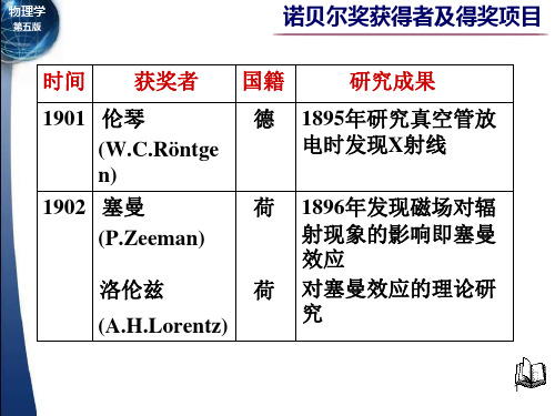
德 1912年发现X射 线的晶体衍射
7
物物理理学学
第第五五版版
诺贝尔奖获得者及得奖项目
时间 获奖者 国籍
研究成果
1915 亨利•布拉格 英
(W.H.Bragg)
劳伦斯•布拉 英 格
(W.L.Bragg)
1917 巴克拉
英
(L.G.Barkla)
利用X射线分析晶体 结构 同上(父子共同)
英 研究大气高层物理性
(E.V.Appieto
质,发现无线电短波
n)
电离层
21
物物理理学学
第第五五版版
诺贝尔奖获得者及得奖项目
时间 获奖者
国籍
研究成果
1948 布莱克
英
(P.M.Blackett)
发展威尔孙云室,在 粒子和宇宙线方面贡 献
1949 汤川秀树 (H.Yukawa)
日 从核力理论基础上 预言介子的存在
时间
获奖者
1909 马可尼 (G.Marconi)
1910
布劳恩 (C.F.Braun) 范德瓦耳斯
(J.D.Van derWaals)
国籍
研究成果
意 发明无线电报和对 发展无线电通讯的 贡献
德 对无线电报的研究 和改进
荷 气体和液体状态方 程的研究
5
物物理理学学
第第五五版版
时间
获奖者
1911 维恩(W.Wien)
17
物物理理学学
第第五五版版
诺贝尔奖获得者及得奖项目
时间 获奖者
国籍
研究成果
1937
戴维孙
美
(C.J.Davisson)
二阶多时滞中立型微分方程的振动性
二阶多时滞中立型微分方程的振动性闫卫平;王兰红【摘要】研究二阶线性中立型微分方程的振动性,对具有多时滞的一类二阶中立型微分方程的振动性进行讨论,利用比较原理将二阶多时滞中立型微分方程的振动性判断转化为判断一阶方程的振动性,这种比较原则最大限度地使研究的二阶方程得到简化。
%To study the oscillation of the second order neutral differential equations with mutiple delays of a class of second order neutral differential equations were discussed .The obtained result were based on the new comparison theorems ,that enable us to reduce the problem ofthe oscillation of the second order equation to the oscillation of the first order equation .T he obtained comparison principles essentially simplifythe examination of the studied equations .【期刊名称】《安徽大学学报(自然科学版)》【年(卷),期】2015(000)003【总页数】4页(P1-4)【关键词】二阶多时滞线性中立型微分方程;比较原理;振动性;非振动性【作者】闫卫平;王兰红【作者单位】山西大学数学科学学院,山西太原030006;山西大学数学科学学院,山西太原 030006【正文语种】中文【中图分类】O175.4讨论二阶多时滞中立型微分方程的振动性.其中:qj(t)∈C([t0,∞)),r(t),pi(t),τi(t),σj(t)∈C1([t0,∞))(i=1,2,…,m;j=1,2,…,n),并且满足假设记方程(1)的解应满足x(t)∈C([Tx,∞)),Tx≥t0 和r(t)z′(t)∈C1([Tx,∞)),并且在[Tx,∞)上满足方程(1).这里只考虑方程(1)的解,对于所有的T≥Tx 满足sup{|x(t)|:t≥T}>0.假设方程(1)拥有这样的解,如果方程(1)的解在[Tx,∞)上有任意大的零解,那么称它为振动的,否则就是非振动的.若方程(1)的所有解都是振动的,那么这个方程就称为是振动的.二阶微分方程在物理、生物、经济等许多方面有重要应用.例如,文献[1-10]讨论了关于二阶中立型微分方程的振动性.在文献[4]中,作者研究了二阶中立型微分方程在文献[7-8]中,作者研究了关于非线性方程的振动性,但是多时滞方程的振动性的研究并不多见.受文献[4]的启发,作者对二阶多时滞中立型微分方程的振动性做了研究,并得到了满意的结果.1 预备知识文中涉及函数不等式都假设它们最终成立,即它们对足够大的t成立.不失一般性,在文中只考虑方程(1)的正解.引理1 设x(t)是方程(1)的一个正解,则对应的函数z(t)最终满足证明若x(t)是方程(1)的一个正解,那么,且由方程(1)知那么(r(t)z′(t))是递减的,最终z′(t)>0或者z′(t)<0.如果设z′(t)<0,那么存在一个常数c,使得r(t)z′(t)≤-c<0,并对该式从t1到t积分,可以得到当t→∞时,有这与z(t)的性质矛盾,从而引理得证.指定这里t是足够大的.2 定理证明定理1 设Q(t)是(3)中定义的且t是足够大的.若一阶多时滞中立型微分不等式没有正解,那么,方程(1)是振动的.证明设x(t)是方程(1)的一个正解,对应的函数z(t)满足z(t)>0,z′(t)>0,(r(t)z′(t))′<0,且有所以,有这里应用了(H3).另一方面,由(1)可知进一步,将(H1)代入计算可得那么所以,有将(H3)代入计算可以得到联合(6)和(8),有将(3)和(5)代入上式可得由引理1知y(t)=r(t)z′(t)>0是递减的,有从而可得联合(9)和(10)可得即这意味着y(t)是(4)的一个正解.这与假设矛盾,从而定理1得证.定理2 设Q(t)是(3)中定义的且t是足够大的.当τi(t)≥t(i=1,2,…,m)时,且一阶微分不等式没有正解,那么方程(1)是振动的.证明设x(t)是方程(1)的一个正解,由引理1和定理1的证明知y(t)=r (t)z′(t)>0是递减的且满足不等式(4).令,且由τi(t)≥t(i=1,2,…,m)知将其代入(4),可以得到w(t)是不等式(11)的一个正解,这与假设矛盾,从而定理2得证.现在考虑τi(t)(i=1,2,…,m)是滞后的时滞,用τ-1i(t)表示它的反函数.定理3 设Q(t)是(3)中定义的且t是足够大的.当τi(t)≤t,τ(t)=min {τi(t)}(i∈{1,2,…,m})时,且一阶微分不等式没有正解,那么方程(1)是振动的.证明设x(t)是方程(1)的一个正解,由引理1和定理1的证明知y(t)=r (t)z′(t)>0是递减的,且满足不等式(4).令,且由τi(t)≤t(i=1,2,…,m)知将上式代入(4),可以得到w(t)是不等式(12)的一个正解.这与假设矛盾,从而定理3得证.参考文献:[1]Grammatikopoulos M K,Ladas G,Meimatidou A.Oscillation of second order neutral delay differential equation[M].Rad Mat,1985[2]Sahine Y.On oscillation of second order neutral type delay differential equations[M].Appl Math Comput,2007,150:697-706.[3]Baculikova J.Oscillation criteria for second order nonlinear differential equations[J].Arch Math,2006,42:141-149.[4]Baculikova J,Dzurina A.Oscillation theorems for second order neutral differential equations[J].Applied Mathematical Modelling,2011,61:94-99.[5]Liu L H,Bai Z.New oscillation criteria for second order nonlinear delay differential equtions[J].Comput Appl Math,2009,231:657-663. [6]Xu R,Xia Y.A note on the oscillation of second order nonlinear neutral functional differential equations[J].Contemp Math Comput Sci,2008(3):1441-1450.[7]Han Z,Li T,Sun S,et al.Oscillation criterial for second order nonlinear neutral delay differential equations[M].Adv Difference Equ,2010:1-23.[8]Dzurina J,Hudakova D.Oscillation criteria for second order delay differential equations[J].Math Bohem,2006:134 31-38.[9]Xu R,Meng F.Oscillation criteria for second order quasi linear neutral delay differential equations[M].Appl Math Comput,2007,192:216-222.[10]Hasanbulli M,Rogovchenko Y.Oscillation criteria for second order nonlinear neutral differential equations[J].Appl Math Comput,2010,。
历年诺贝尔生理医学奖及化学奖获奖者整理
历年诺贝尔生理医学奖及化学奖获奖者整理历年诺贝尔生理医学奖获奖者:1901年,埃米尔·阿道夫·冯·贝林(德国)。
利用血清疗法治疗白喉。
1902年,Ronald Ross(英国)。
关于疟疾的研究。
1903年,尼尔斯·吕贝里·芬森(丹麦)。
利用光辐射治疗狼疮。
1904年,巴甫洛夫(俄国)。
在神经生理学方面,提出了著名的条件反射和信号学说。
1905年,R.柯赫(德国)。
关于结核方面的研究和发现。
1906年,C.高尔基(意大利),桑地牙哥·拉蒙卡哈(Santiago Ramón y Cajal,西班牙)。
关于神经系统结构的研究。
1907年,Charles Louis Alphonse Laveran(法国),发现原生动物在引起疾病中的作用。
1908年,Ilya Ilyich Mechnikov(俄国),保罗·埃尔利希(德国)。
关于免疫方面的研究。
1909年,埃米尔·特奥多尔·科赫尔(Emil Theodor Kocher)(瑞士)。
关于甲状腺生理学,病理学和外科学方面的研究。
1910年,艾布瑞契·科塞尔(Albrecht Kossel)(德国)。
关于细胞化学尤其是蛋白质和核酸方面的研究。
1911年,Allvar Gullstrand(瑞典)。
关于眼睛屈光学方面的研究。
1912年,Alexis Carrel(法国)。
关于血管缝合以及血管和器官移植方面的研究。
1913年,Charles Robert Richet(法国)。
关于过敏反应的研究。
1914年,Robert Bárány(奥地利)。
关于内耳前庭装置生理学及病理学方面的研究。
1915年-1918年,未颁奖,奖金划拨到生理医学奖专门的基金上。
1919年,Jules Bordet(比利时)。
关于免疫方面的研究。
1920年,Schack August Steenberg Krogh(丹麦)。
核磁共振谱 红外光谱 质谱

The Noble Prize in Physics 1943 美籍德国人O.Stern 因发展分子束的方法 和发现质子磁矩获得 了1943年诺贝尔物 理学奖。 Otto Stern Carnegie Institute of Technology Pittsburgh, PA, USA
The Noble Prize in Physics 1952 1946年,美籍科学家Bloch和Purcell首次观测 到宏观物质核磁共振信号,他们二人为此获 得了1952年诺贝尔物理学奖。
1
即:
1
(为自旋核高能态寿命)
核磁共振的基本原理
弛豫过程的分类 能级回到低能级。该能量被转移至周围的分子(固体的晶 格,液体则为周围的同类分子或溶剂分子)而转变成热运 动,即纵向驰豫反映了体系和环境的能量交换; 自旋—自旋驰豫,也称为横向驰豫,这种驰豫并不改变 低能态和高能态之间粒子数的分布,但影响到具体的核 在高能级停留的时间。
8
两种能级:m=1/2, m=-1/2上数目之比:
6.626 34 100.0 6 E h E E i j 10 23 10 i exp exp exp exp kT kT kT 1.3806610 298 j 0.999984
The Nobel Prize in Physiology or Medicine 2003 2003年诺贝尔生理或医学奖授予美国的保罗· C· 劳特伯(Paul C. Lauterbur)和英国的皮特· 曼斯菲尔德(Peter Mansfield), 因为他们发明了磁共振成像技术(Magnetic Resonance Imaging, MRI)。该项技术可以使 人们能够无损伤地从微观 到宏观系统地探测生物活体的结构和功能,为医疗诊断和科 学研究提供了非常便利的 手段。
劳伦斯利弗莫尔国家实验室详细资料大全
劳伦斯利弗莫尔国家实验室详细资料大全劳伦斯利弗莫尔国家实验室(Lawrence Livermore National Laboratory,LLNL),美国著名国家实验室之一,位于美国旧金山湾区利弗莫尔(Livermore),隶属于美国能源部的国家核安全局(NNSA),现由劳伦斯利弗莫尔国家安全机构(LLNS,由加州大学等机构联合构成)负责运行。
劳伦斯利弗莫尔国家实验室建立于1952年,最早是劳伦斯伯克利国家实验室设在加州旧金山湾区利弗莫尔(Livermore)的分支实验室,由加州大学伯克利分校物理学教授欧内斯特·劳伦斯(诺贝尔奖得主)、爱德华·泰勒(氢弹之父)共同建立。
实验室早期由加州大学全权负责运行,2007年后改由LLNS负责运行,主要负责研发包括核武器在内的美国国防科技。
劳伦斯利弗莫尔国家实验室发现或参与发现了6种化学元素(113号- 118号元素)。
值得注意的是,加州大学伯克利分校和劳伦斯伯克利国家实验室此前共同发现或参与发现了16种化学元素,后化学元素的研究项目被劳伦斯利弗莫尔国家实验室所继承。
基本介绍•中文名:劳伦斯利弗莫尔国家实验室•外文名:Lawrence Livermore National Laboratory•建立时间:1952年•隶属:美国能源部•运行单位:LLNS(加州大学等共同构成)•地址:美国加州旧金山湾区•现任主任:Bill Goldstein历史沿革,人员机构,科研成果,化学元素,超级计算机,美国国家点火装置,高安保级别核材料,科研合作,获奖情况,历史沿革劳伦斯利弗莫尔国家实验室(Lawrence Livermore National Laboratory,LLNL)于1952年建立于美国加州旧金山湾区的利弗莫尔(Livermore),由加州大学伯克利分校物理学教授欧内斯特·劳伦斯、爱德华·泰勒(氢弹之父)共同建立。
最初名叫“加州大学放射实验室-利弗莫尔分部”(University of California Radiation Laboratory at Livermore),是位于加州大学伯克利分校的“加州大学放射实验室”的分支实验室,隶属于美国能源部(DOE),由加州大学具体负责运行。
带有强迫项的二阶拟线性微分方程的振动准则
带有强迫项的二阶拟线性微分方程的振动准则王培颖【摘要】In this paper,by using integral averaging functions of the formu(t)and the generalized Riccati technique,new interval oscillation criteria areestablished for forced second-order quasi-linear differential equations of the form p (t)y′(t)α-1 y′(t) ( )′+q(t)q(t)β-1 y (t)=e(t).We drop the restriction “φ′(t)≥0”in some existing results.%主要利用一元函数 u(t)型积分平均辅助函数和广义 Riccati 变换技巧,建立带有强迫项的二阶拟线性微分方程 p (t)|y′(t)|α-1 y′(t)()′+q(t)|y (t)|β-1 y (t)=e (t)的新的区间振动准则,去掉了某些已有结果中关于“φ′(t)≥0”的限制。
【期刊名称】《德州学院学报》【年(卷),期】2015(000)004【总页数】5页(P24-28)【关键词】微分方程;区间振动准则;Riccati 变换技巧;强迫项【作者】王培颖【作者单位】广东技术师范学院天河学院,广州 510540【正文语种】中文【中图分类】O175考虑带有强迫项的二阶拟线性微分方程(p(t)|y′(t)|α-1y′(t))′+q(t)|y(t)|β-1y(t)=e(t),t≥t的振动性,其中p,q,e∈C([t0,∞),R),p(t)>0,0<α≤β(α,β是常数),称函数 y(t)∈C1([Ty,∞),R),Ty≥t0,是方程(1)的解,如果p(t)|y′(t)α-1|y′(t)∈C1(Ty,∞)且满足(1)式.主要考虑方程(1)的非平凡解y(t),即sup{|y(t)|:t≥T}>0,T≥Ty,如果它有任意大的零点,方程(1)的非平凡解y(t)称为振动的;否则,称之为非振动的.如果它的所有非平凡解都是振动的,方程(1)称为振动的.当0<α=β时,方程(1)转化为半线性微分方程(p(t)|y′(t)|α-1y′(t))′+q(t)|y(t)|α-1y(t)=e(t≥t当0<α<β时,方程(1)是超半线性微分方程.方程(2)和它的特殊情形(没有强迫项)(p(t)|y′(t)|α-1y′(t))′+q(t)|y(t)|y(t)=0,t≥t的振动性已经被许多学者广泛的研究,可见Elbert[3],Li和Yeh[4].拟线性微分方程(3)和线性微分方程具有类似的性质.例如,当 w=时,方程(3)可转化为方程(4)和α+1阶泛函与线性振动理论中的经典Riccati方程和二次泛函起着相同的作用.当α=1时,方程(2)转化为带有强迫项的线性微分方程对于方程(6),1999年Wong[5]得到下面结果定理1 如果对任意T≥t0,存在T≤s1<t1≤s2<t2,使得令D(si,ti)={u∈C1[si,ti]:u(t)≠0, u( si)=u( ti)=0};i=1,2假定存在u∈ D( si,ti),使得则方程(6)是振动的.上述定理改进了没有强迫项的微分方程的结论.2002年,Li和Cheng [6]用类似的方法和一个正的、非减的函数φ∈C1([t0,∞),R)可以将定理1的结论推广到方程(2)的振动性.定理2 如果对任意T≥t0,存在T≤s1<t1≤s2<2,使得假定存在H∈D(si,ti)和一个正的、非减的函数φ∈C1([t0,∞),R)使得则方程(2)是振动的.当α=1,φ(t)=1,H(t)=t)时,(8)式转化为(7)式.(8)式和(5)式没有联系,并且定理2不能应用于α>1的情形.2007年,Zheng和Meng[7]将定理2推广到方程(1).定理3 如果对任意T≥t0,存在T≤s1<t1≤s2<t2,使得假定存在H∈si,ti)和一个正的、非减的函数φ∈C1([t0,∞),R)使得其中,约定00=1,则方程(1)是振动的.上述定理1-3所用的积分平均辅助函数为一元的.1999年,Manojlovic[8]利用Philos[9]提出的二元函数H(t,s)型积分平均辅助函数,研究了方程(3)的振动性,其中的一个结果如下.定理4 假设存在一个定义在 D={(t,s):t≥s≥t0}→R上的连续函数H,使得H(t,t0)=0,t≥t0,H(t,s)>0,(t,s)∈D.是定义在D上的非负连续函数.如果存在一个正的、非减的函数ρ∈C1([t0,∞),R),使得成立,则方程(3)是振动的.2001年,Wang[10]将定理4中的限制“ρ′(t)≥0”去掉.2004年,Wang和Yang[11]利用二元函数H(t,s)型积分平均辅助函数,研究了方程(3)的区间振动性,其中的一个结果如下.定理5 假设存在c∈(a,b),ρ∈([t0,∞),(0,∞)]),使得则方程(3)的每一个解在(a,b)上至少有一零点.将利用一元函数u(t)型积分平均辅助函数,建立方程(1)的新的区间振动准则.首先给出一个不等式,可见文献[29].引理1 假设X≥0,等号成立有且只有 X=Y.下面给出主要结果.定理6 如果对任意T≥t0,存在T≤s1<t1≤s2<t2,使得令D(si,ti)={u∈ C1[si,ti]:uα+1(t)>0,t∈( si,ti),u(si)=u(ti)=0};i=1,2假定存在H∈D(si,ti)和一个函数φ∈C1([t0,+∞),(0,+∞))使得p(t)dt>0,i=1,2其中约定00=1,则方程(1)是振动的.证明反证法.假设方程(1)有非平凡非振动解 y(t),t∈[t0,∞),则存在T0≥t0使得当t≥Ty(t)≠0.不妨设y(t)>0.令对(10)式求导并利用方程(1)得由假设取t1>s1≥t0,因此在I1=[s1,t1],e(t)≤0,令F′(x)=0,得所以由(11)(12)得即把(13)式两边同乘以 Hα+1(t)并从si到ti积分,而且H(si)=H(ti)=0,得到令据引理1所以∫tisiφ(t) Q e(t) H α+1(t)dt≤∫ tisit)p(t)即当i=1时(14)与(9)矛盾,同理当 y(t)<0.t≥T0>t0,做和(10)式相同的Riccati变换得当 i=2时与(9)式矛盾,定理得证.推论1 若在定理6中令φ(t)≡1,式子(9)变为Qi(H)=∫tisi[Qe(t)Hα+1(t)-p(t)则方程(1)是振动的.推论2 若在定理6中令φ(t)≡1,α=β>0,式子(9)变为Qi(H)=∫tisi[q(t)Hα+1(t)-p(t)则方程(2)是振动的.注定理6去掉了定理2和定理3中关于“φ′(t)≥0”的限制.例考虑带有强迫项的拟线性微分方程方程其中λ,γ都是常数,且λ,γ>0在定理6中取,则取,对任意T≥1,当nπ=2kπ≥T,s1=2kπ,t1=(2k+1)π,于是由定理6得故即因此当时.同理,取s2=(2k+1)π,t2=(2时.所以据定理6得当0<γ<时原方程是振动的.[1]parisonAnd Oscillation Theory of Linear Differential Eq uations[M].New York:Academic Press,1968.[2]燕居让.常微分方程的振动理论[M].太原:山西教育出版社,1992.[3]A.Elbert.A half-linear second order differential equation,Colloq.Math.Soc.Janos Bolyai:Qual itative Theory of Differential Equations[J].Szeged,1979:153-180.[4]H.J.Li,CC.Yeh.Sturmian comparison theorem for half-linear second-order differential equations[J].Proc.Royal Soc. Edinburgh 125A,1995:1193-1204.[5]J.S.W.Wong.Oscillation criteria forA second-order linear differential equation[J].J.Math.Anal.Appl.,1999,231:235-240. [6]W.T.Li,S.S.Cheng.An oscillation criterion for nonhomogeneous half-linear differential equations[J].Appl.Math.Lett.2002,15:259-263.[7]Zhaowen Zheng,Fanwei Meng.Oscillation criteria for forced second-order quasi-linear differential equations[J]put.Modelling,2007,45:1-2,215-220.[8]J.V.Manojlovi’c.Oscillation criteria for second-order half-linear differential equations[J]put.Modelling,1999,30:109-119.[9]Ch.G.Philos.Oscillation theorems for linear differential equations of seco nd order[J].Arch.Math.(Basel),1989,53:482-492.[10]Qi-Ru Wang.OscillationAndAsymptotics for second-order half-linear differential equations[J]put.,2001,122:2,253-266. [11]Qi-Ru Wang,Qi-Gui Yang.Interval criteria for oscillation of second-order half-linear differential equations[J].J.Math.Anal.Appl.,2004,291:1,224-236.[12]Y.G.Sun.New Kamenev-type oscillation criteria for second-order nonlinear differential equations with damping[J].J.Math.Anal.Appl.,20 04,291:341-351.[13]Qi Long,Qi-Ru Wang.New oscillation criteria of second-order nonlinear differential equations[J]put.,2009,212:2,35 7-365[14]Yin-Lian Fu,Qi-Ru Wang. Oscillation criteria for second-order nonlinear damped differential equations.Dynam.SystemsAppl.18(200 9),no.3-4,375-391.[15]D.Cakmak,A.Tiryaki,Oscillation criteria for certain forced second-order nonlinear differential equations[J].Appl.Math.Lett.,2004,17: 275-279.[16]J.Jaros,T.Kusano,A Picone type identity for second order half-linear differential equations[J].Acta enian. 1999, 68 (1):137-151.[17]J.Jaros,T.Kusano,N.Yoshida.Generalized Picone’s formulaAnd forced o scillation for in quasilinear differential equations of the secondorder[J].Arch.Math.(Bero),2002,38:53-59.[18]A.Wintner.A criterion of oscillatory stability[J].Quart.Appl.Math.,1949,7: 115-117.[19]I.V.Kamenev.Integral criterion for oscillation of linear differential equati ons of second order[J].Mat.Zametki,1978,23:249-251.[20]parison theorems for linear differential equations of se cond order[J].Proc.Amer.Math.Soc.,1962,13:603-610.[21]Q.Kong.Interval criteria for oscillation of second-order linear differential equation[J].J.Math.Anal.Appl.,2001,258:244-257. [22]H.L.Hong,W.C.Lian,C.C.Yeh.The oscillation of half-linear differential equations withAn oscillatory coefficient[J]put. Modelling,1996,24:77-86.[23]J.S.W.Wong.Second order nonlinear forced oscillations[J].SIAM J.Math. Anal.,1988,19:667-675.[24]Qi-Ru Wang.Oscillation criteria for nonlinear second order damped differentia l equations[J].Acta Math.Hungar.,2004,102:117-139.[25]Qi-Ru Wang.Interval criteria for oscillation of certain second order nonlinear d ifferential equations[J].Dynam.Cont.Discrete Impulsive Syst.SeriesA:Math.A nal.,2005,12:769-781.[26]Qi-Ru Wang.Interval criteria for oscillation of second-order nonlinear differential equations[J]put.Appl.Math.,2007,205:1,2 31-238.[27]H.W.Wu,Q.R.Wang,Y.T.Xu.OscillationAndAsymptotics for nonlinear seco nd-order differential equations[J].Comput.Math.Appl.,2004,48:61-72. [28]Q.G.Yang.Interval oscillation criteria forA forced second order nonlinea r ordinary differential equations with oscillatory potential[J].Appl.Math.Co mput.,2003,135:49-64.Key words:differential equations; interval oscillation criteria; generalized ric cati transformation; forcing term。
- 1、下载文档前请自行甄别文档内容的完整性,平台不提供额外的编辑、内容补充、找答案等附加服务。
- 2、"仅部分预览"的文档,不可在线预览部分如存在完整性等问题,可反馈申请退款(可完整预览的文档不适用该条件!)。
- 3、如文档侵犯您的权益,请联系客服反馈,我们会尽快为您处理(人工客服工作时间:9:00-18:30)。
OSCILLATION THEOREMS FOR SYSTEMS OFLINEAR DIFFERENTIAL EQUATIONSBYZEEV NEHARI(')1. The systems to be considered in this paper are of the form(1.1) / = Ay,where A = A(x) is a continuous n x « matrix on an x-interval F, and y is an «-dimensional column vector. We shall assume that the elements of A are real, and we shall consider only real solution vectors of (1.1). This is not an essential restric-tion since, in the complex case, (1.1) can be replaced by an equivalent real system with a 2« x 2« coefficient matrix.We shall say that a nontrivial solution vector y = (yx,..., yn) of (1.1) is oscillatory on F if each of its components takes the value zero at some point of R, i.e., yk(xk) = 0, xk e R, k = 1,..., «. The system (1.1) itself will be said to be oscillatory if it possesses at least one oscillatory solution vector. If there is no such solution vector, i.e., if every nontrivial solution vector has a component which does not vanish on F, the system will be said to be nonoscillatory on R.In a recent paper by B. Schwarz [16], systems with the latter property are called "disconjugate", rather than "nonoscillatory", and a word of justification for this change of terminology is in order. The term "disconjugate", as introduced by Wintner [21], refers to the absence of a conjugate point in the sense of Jacobi, and thus originally applied only to selfadjoint equations and systems [3], [4], [14], [15], [19], [20]. However, this concept generalizes in a natural way to general «th order differential equations [1], [8], [9], [10], [13], [17], [18] and thus also to systems which are equivalent to such equations. In all these cases, the right con-jugate point r¡(x0) of x0 (■n(x0)>x0) is a continuous function of x0, and the left conjugate point of ^(x0) coincides with x0 [17], [18]. In the case of a system which can be reduced to an nth order equation, -n(x0) c an be defined in the following way : there exists a solution vector of (1.1) such that every component of y vanishes either at x0 or at r¡(x0), and -n(x0) i s the smallest number with this property. It can then be shown that r¡(x0)=infb, where b is such that the system is oscillatory in [x0, b) [9], [13], [17].In the case of a general system (1.1), the conjugate point may be defined in the same way, but it is in general not true that ry(x0) = £(x0), where £(x0)= m^ b, andReceived by the editors February 6, 1968 and, in revised form, August 21, 1968.(') Research sponsored by the Air Force Office of Scientific Research, Office of Aerospace Research, United States Air Force, under AFOSR Grant No. 62-414.339340 ZEEV NEHARI [May[x0, b) is an interval of oscillation of the system. That this can happen even in the case of a 2 x 2 matrix A, is shown by the following simple example. IfA = (a a\ = 2x 2(x-l)\t tJ' " x2 + (x-l)2' T_x2 + (x-l)2'equation (1.1) has the two independent solution vectors (x2, (x-1)2) and (1, — 1). The general solution is thus (ax2+ß, a(x— l)2—j8), where a, ß are constants, and it is easily seen that (x2, (x—l)2) is the only oscillatory solution of the system. Accordingly, the point x=l is the only point which possesses a conjugate point. On the other hand, £(x0) =1 for all nonpositive x0. Moreover, if we set %(x0) = sup a, where the system is oscillatory in (a, x0], we have \(xQ) = 0 for all x^ 1, and this shows that £[Ç(x0)] =1 ¥= x0 if x0 > 1. It would therefore hardly be appropriate to call £(x0) the conjugate point of x0. Accordingly, it seems preferable to say that the system is nonoscillatory in (x0, ri(xQ)), r ather than disconjugate.We introduce here yet another concept which is closely related to nonoscillation, and which has the merit that it can be defined without reference to the components of the solution vectors. We shall say that the system (1.1) is suborthogonal on R if, for any nontrivial solution vector y, and for any s e R, t e R,(1.2) y(s)y(0 > 0.In the case of a 2 x 2 matrix, suborthogonality implies nonoscillation ; indeed, if the two components of y vanish at s and /, respectively, we evidently have y(s)y(0 = 0.It may be noted that, if C is a constant orthogonal matrix the system(1.3) w' = CAC-^is suborthogonal if the same is true of the system (1.1). Indeed, the general solution of (1.3) is of the form Cy, where y is the general solution of (1.1), and the assertion follows from the fact that [Cy(s)][Cy(0]=y(s)y(0- Nonoscillation is in general not preserved if the coefficient matrix A is replaced by CAC~X. However—and this points up the close relation between the concepts of nonoscillation and sub-orthogonality—if the system (1.3) is nonoscillatory on R for all constant orthogonal matrices C, then it is also suborthogonal on this interval. To establish this assertion, suppose (1.1) has a nontrivial solution vector y for which y(s)y(0 = 0, s e R, t e R. If we determine the constant orthogonal matrix C so that the vector Cy(s) has the components (||y(s)|| 0,..., 0), it follows from 0=y(s)y(i)= [Cy(s)][Cy(0] that the first component of Cy(0 is zero. Hence, (1.3) has a solution vector w=Cy all of whose components vanish at either s or t and it follows that (1.3) is oscillatory.The suborthogonality of the system (1.1) can also be expressed in terms of a fundamental (i.e., nonsingular) solution matrix Y of the matrix-matrix equation(1.4) Y'= AYcorresponding to (1.1). Since the general solution of (1.1) is of the form y= Ya, where a is an arbitrary constant vector, condition (1.2) is equivalent to aY*(s) Y(t)a1969] OSCfLLATION THEOREMS FOR DIFFERENTIAL EQUATIONS 341>0, i.e., to the condition that the symmetric part of the matrix Y*(s)Y(t) he positive-definite for all s e R, te R. In particular, if we choose a fundamental solution Fs of (1.3) which reduces to the unit matrix 7 for x=s, the condition becomes aFs(Oa>0- With the help of this version of condition (1.2) it is easy to establish the following property of suborthogonal systems.If the system (1.1) is suborthogonal, so is the adjoint system(1.5) w' = -A*w.Indeed, if the matrix Ws(x) is the fundamental solution (with Ws(s) = I) of the matrix-matrix equation corresponding to (1.5), we have(W* Ys)' =- W*A Y+ W*A Y =0and therefore W*YS=I. Hence, if yS is an arbitrary constant vector, and we set a= Ys~\t)ß= W*(t)ß, we have ßWs(t)ß=ßW*(t)ß = aYs(t)a>0. Since s, t and the constant vector ß were arbitrary, the assertion follows.2. The principal aim of this paper is to obtain conditions—expressed in terms of the coefficient matrix—which guarantee the nonoscillation of the system (1.1) on a given interval. All these conditions will follow from two basic inequalities, which we state here in the form of a theorem.Theorem 2.1. Let y and w be nontrivial solution vectors of the systems:(2.1) y' - Ay,(2.2) w' = Bw,respectively, where the nxn matrices A, B are continuous on the interval [a, b]. If u, v are the unit vectors(2.3) u = y/\\y\\, v = w/\\w\\and C is an arbitrary constant orthogonal matrix, then(2.4) |arc sin [u(b)Cv(b)]~arc sin [zz(a)Ct<a)]| ¿ f (\\A\\ +\\B\\) d x,Jawhere \\A\\ denotes the norm sup|ja[| =1 \\Aa\\.If one of the systems (2.1), (2.2) is oscillatory on [a, b], (2.4) can be replaced by the stronger inequality(2.5) |arc sin [u(b)Cv(b)]\ + |arc sin [w(a)Ci<a)]| ^ f (||^|| + ||F||) dx.JaProof. Differentiating (2.3), we obtain"'=//lbll-j0y)/bll3,and a similar expression for v'. In view of (2.1) and (2.2), this leads to(2.6) u' = Au—u(uAu)and(2.7) v' = Bv-v(vBv).342 ZEEV NEHARI [May If C is a constant orthogonal matrix, we have (uCv)' = u'Cv + v'C*u and thus, by (2.6) a nd (2.7),(2.8) iuCv)' = [Cv-(uCv)u]Au+[C*u-(uCv)v]Bv.Hence, since u and v are unit vectors,I («co'| s \\Cv-(uCv)u\\-\\a\\ + \\c*u-(uCv)v\\-\\b\\.Because ofandthis implies :|Ct;-(uC0w||2 = \\Cv\\2-(uCv)2 = 1-(«C02\C*u-(uCv)v\\2 = ||C*m||2-(mC02 = l-(wC02,f)Q\ ("CO' < mil , h f ill(2-9) (1-(«C0T2- ^ll + ^ll'and an integration establishes (2.4).We now turn to the proof of inequality (2.5). Since uCv = vC*u, we may assume without loss of generality that w (and thus also 0 is oscillatory on [a, b]. If vx,.. ,,vn are the components of v, there will thus exist a set of points xx,..., xn in [a, b], containing at least two different points (since otherwise w would reduce to the trivial solution), such that t^(xk) = 0, k = l,..., n. Evidently, the vector Cv(xk) is not changed if the elements cik, i=l,..., n in the kth column of the matrix C are replaced by different numbers. We shall take advantage of this fact by substituting — c ik for clk (i= 1,..., n), and we note that this change does not affect the orthogonal character of the matrix. Proceeding from a to b, and making this change whenever a point xk is crossed, we obtain a matrix function C(x) which is constant and orthogonal in the intervals between adjacent points xk. By the construction of C(x), the vector function C(x)zz(x) is continuous on [a, b], and we evidently have C(b) =- C(a) = - C.In any interval between adjacent points xk we may use (2.9) with C(x) substituted for C. We integrate, and add up the contributions from all the intervals making up [a, b]. Since C(x)v(x) is continuous, and since C(b)= —C(a)= — C, we obtain|arc sin [u(b)Cv(b)] +arc sin [u(a)Ctz(a)]| S \ (\\A\\ +\\B\\) d x.JaCombining this with (2.4), we obtain (2.5). It is easy to see that this argument remains valid if some (or even all) of the points xk coincide with either a or b.In the special case in which C is a diagonal matrix whose elements ckk a re either 1 or — 1, the continuity of C(x) is not affected by changing ckk into — ckk at a point at which the kth component of either u or v is zero. In order to obtain inequality (2.5) it is therefore sufficient to assume that, for each k (k = l,..., ri),1969] OSCILLATION THEOREMS FOR DIFFERENTIAL EQUATIONS 343the kth component of at least one of the vectors y, w vanishes on [a, b]. If, for x=a, we take C to be the unit matrix, this leads to the following result.Theorem 2.2. Let y, w, A, B, u, v have the same meaning as in Theorem (2.1). If, for each k (k = 1,..., «), the kth component of at least one of the vectors y, w vanishes at a point of [a, b], then(2.10) |arc sin [u(b)v(b)]\ + |arc sin [u(a)v(a)]\ ^ fJa Mil +11*11)<fa.3. As a first application of Theorem 2.1 we derive the following sufficient condition for suborthogonality.Theorem 3.1. If, for some continuous real function p.=p.(x) on [a, b], we have (3.1) f \\A+p.I\\dx<jthen the system (2.1) is suborthogonal on [a, b]. The constant -n/2 in (3.1) is the best possible; in fact, the conclusion does not necessarily hold if the sign of equality is permitted in (3.1).Proof. We use (2.4), with F=0 and C=7. Since (2.2) is solved by an arbitrary constant vector, v may be taken to be an arbitrary constant unit vector. If a^s <t^b, and we set v = u(t), (2.4) becomes(3.2)- arc sin [u(s)u(t)]\ ^ Mil ax = \\A\\ d x.Js JaIf (2.1) is not suborthogonal on [a, b], there exist s, t e [a, b] such that u(s)u(t) = 0. In this case we thus must have 7r/2£j"a \\A\\ d x. If p.=0, this conflicts with (3.1) and thus proves Theorem (3.1) in this particular case. The case of a general con-tinuous function p. is easily reduced to the case p = 0, since the general solution of the system o' = (A+Ifi)o is of the form o=gy, where g(x) is the scalar function exp {/* p. dx) and y is the general solution of (2.1). We have o(s)o(t)=g(s)g(t)x [y(s)y(t)] and, since g #0, the system a=(A+p.I)o is suborthogonal if, and only if, the same is true of the system (2.1).To show that the constant in Theorem 3.1 is the best possible, we set n = 2m, where m is a positive integer, and we consider the coefficient matrix A whose elements aik are defined as follows: ak.k + x=l, k= 1,...,«— 1, anX = (— l)m; all other elements of A are zero. It is easily confirmed that the system (2.1) associated with this matrix has a solution vector y=(yx,.. .,y2m) with y2k+x = (-l)k sin x, k = 0,..., m-l, and y2k = (-l)k + 1c os x, k=l,.. .,m. Accordingly, we have y(0)y(tr/2) = 0, i.e., the system is not suborthogonal on [0,7r/2]. On the other hand, it is easily confirmed that Mil "*h and tnusI*'2 7TA\dx~\344ZEEV NEHARI[MayThis shows that (3.1) (with the particular choice p=0) is the best possible condition of its kind and that suborthogonality does not necessarily obtain if the sign of equality holds in (3.1). We also note for further reference that the exhibited solution vector is oscillatory on [0, tt/2].Turning now to criteria for nonoscillation, we set B=0, C=I in (2.5) and, as before, we identify the arbitrary constant unit vector v with u(a). An application of Theorem 2.1 then leads to the following result.Theorem 3.2. If the solution vector y of (2.1) is oscillatory on [a, b], then (3.3) ?+arcsin ,, ^f^' S f \\A\\ dx.2 || y(a) I || y(Zz) || JaAs an immediate corollary of this result we find that the condition j"a \\A\\ d x <rr/2 is sufficient to guarantee the nonoscillation of the system (2.1) on [a,b]. However, this criterion can be given a more general form with the help of an arbitrary diagonal nxn matrix P, whose diagonal elements pkk are continuously differentiable and do not vanish on [a, b]. If w=Py and y is a solution of (2.1), the vector w is a solution of(3.3) w' = (PAP-^P'P-^wand, as remarked by B. Schwarz [16], the system (3.3) is nonoscillatory on an interval if and only if the same is true of the system 2.1 ; indeed, if yk and wk are the components of y and w, respectively, then wk=pkkyk, and p^^O. We thus have the following result.Theorem 3.3. Let P be a diagonal nxn matrix whose diagonal elements are con-tinuously differentiable and do not vanish on [a, b], and let A be a continuous nxn matrix on this interval. If(3.4) f \\PAP-1+P'P-1\\ dx < ^.then the system (2.1) is nonoscillatory on [a, b]. The constant tt/2 in (3.4) is the best possible, and the conclusion does not necessarily hold if the sign of equality is per-mitted in (3.4).A weaker form of condition (3.4) (with the constant 1 instead of tt/2) was recently obtained by W. J. Kim [7]. (For nonoscillation criteria of a different type see [11], [12], [16].) The sharpness of (3.4) can be verified (for F=/), with the help of the same example which was used to show that Theorem 3.1 is the best possible of its kind.4. The presence of the n arbitrary functions in the main diagonal of P lends a great deal of flexibility to condition (3.4). For a given A, the best choice of F would be that which minimizes the integral on the left-hand side (and thus increases the interval to which the condition may be applied). Since the resulting variational problem will in general present great technical difficulties, it will often be more1969] OSCILLATION THEOREMS FOR DIFFERENTIAL EQUATIONS 345rewarding to choose a matrix F of simple type which depends on some arbitrary parameters, and then to find the best criterion obtainable in this way.We shall illustrate this method in the case of a system (2.1) which is equivalent to the «th order scalar differential equation(4.1) oM + r(x)o = 0,where v(x) is continuous on the interval [a, b]. If A is the « x « matrix whose only nonzero elements aik are afc(fc+1=l, fe=l,...,n—1 and anX=-r, the solution vector y of (2.1) has the components o,o',..., <7(n_1), where o is the solution of (4.1). The nonoscillation of the system is thus equivalent to the condition that, for any solution o of (4.1), at least one of the functions o, o ,..., a*»-1' does not vanish in the interval in question. An equation with this property is said to be disfocal on the interval [13]. It may be noted that, by Rolle's theorem, a real disfocal equation is a fortiori disconjugate, i.e., none of its solutions can have more than «— 1 zeros on the interval.Theorem 4.1. Let R be a closed x-interval and let S be a measurable subset of R ofLebesgue measure p.(S). Ifr(x) is continuous on R, ifr(x)j±0 except on a null set, and if(4.2) sup M S)]""1 Js s \r\ d x < (n-iy-^J,then equation (4.1) is disfocal on R. The constant in (4.2) is the best possible.If r is of constant sign and |r| is monotonie on F, the expression (4.2) can be simplified. For instance, if |r| is nondecreasing and F is the interval [a, b], (4.2) may evidently be replaced by the condition(4.3) sup (c-a)""1 Í |z-|o-x < («-l)""1^)", ce[a,b].To prove Theorem 4.1, we use a constant diagonal matrix F. If we setpkk = ßn~k, k = l,.. .,n, where ß is a positive constant, the matrix PAP~1 = (bik) has the elements bktk +i=ß, k=l,.. .,«-1, bnA= -rß~n + 1, and all the other elements bik are zero. It is easy to see that\\PAP-1+P'P-1\\ = HF^P-1!! = max [ß, \r\ß~n+1],and we may therefore conclude from Theorem 3.3 that the system associated with the coefficient matrix A is nonoscillatory on F (and, therefore, the equation (4.1) is disfocal on F) if" {max[ß,\r\ß-n+1]}dx<~; z.JrIf S denotes the subset of F on which \r\^ßn, this may be written in the form(4.4) ßp.(S)+ß~n + 1 f \r\dx <Jb-s346ZEEV NEHARI[MayA simple approximation argument shows that it is sufficient to treat the case in which r is not constant on any subinterval of R. In this case it is possible to choose ß in such a way that(4 5Ï _£L _ Sn-s\r\dx( - ' n-\~ p(S)Indeed, the set S depends on ß, and it is easy to see that the right-hand side of (4.5) varies continuously from 0 to co if ßn decreases from max |z-| to 0. Hence, there must exist a positive ß for which (4.5) holds. For this particular value of ß, the left-hand side of (4.4) takes the form(4.6) ^-r {(«- IMS)]""1 £ s \r\ dx}1'",and condition (4.4) will thus certainly be satisfied if (4.2) holds. This completes the proof of Theorem 4.1.To show that the constant in (4.2) is the best possible, we consider the equationa(2m)-(-l)m(7 = 0on the interval [0, tt/2]. The solution sin x of this equation, as well as all its deriva-tives, vanish at either 0 or 7r/2, and the equation is thus not disfocal on [0,7r/2]. On the other hand,maxc""1 j |r| dx = maxcn_1l^-c) = («-l)n_1l^-J , (zz = 2zw)and this shows that the constant in condition (4.2) (which in this case is equivalent to condition (4.3)) cannot be improved upon.5. Finally, we give a simple example which illustrates the use of Theorem 2.2. We take B to be a matrix whose only nonzero elements bik a ppear in the zzth c olumn, and we set bx¡n = b2¡n= ■ ■■=bm¡n = c (lSmSn-l), where e is a small positive number, and 6…+i,» = • • • = èn,… = 0. We have ||5|| =e\/m, and it is easily confirmed that the system (2.2) associated with this matrix B has the solution vector w = (e(x-xx), c(x-x2),.. .,£(x-xm), cm +x,..., cn_!, 1), where xx, ...,xm, cm +x, . .., cn_x are arbitrary constants. If xr e [a, b], r= 1,..., zzz, the first m components of w have zeros in [a, b], and Theorem 2.2 can be applied if y = (yi,..., y…) is a solution vector of (2.1) whose components ym+x,..., yn vanish at points of [a, b]. For £->0, we have ||5||->0 and zz = w/||w|| tends to a constant unit vector f = (izl5..., vn) with vx = v2 =■ • • =zzm=0, vk = ak, k = m + l,..., n. This leads to the following result.Theorem 5.1. Let y = (yx,.. .,yn)be a solution vector of the system (2.1). If each of the components ym +i, ■ ■-, yn (i=mSn-l) vanishes at some point of the interval [a, b], then1969] OSCILLATION THEOREMS FOR DIFFERENTIAL EQUATIONS 347(5.1)■ST -hCarc sin £ uk(b)ak + arc sin ¿^ uk(a)ak S \A\dx k=m+l k=m+l Jawhere u = (ui.«n)=jVII>i> and tne ak are such that a2 + 1+ • • • +a2= 1 and are otherwise arbitrary.References1. J. H. Barrett, Fourth order boundary value problems and comparison theorems, Cañad. J. Math. 13 (1961), 625-638.2. E. A. Coddington and N. Levinson, Theory of ordinary differential equations, McGraw-Hill, New York, 1955.3. P. Hartman, Ordinary differential equations, Wiley, New York, 1964.4. P. Hartman and A. Wintner, On disconjugate differential systems, Cañad. J. Math. 8 (1956), 72-81.5. R. W. Hunt, The behavior of solutions of ordinary, self-adjoint differential equations of arbitrary even order, Pacific J. Math. 12 (1962), 945-961.6. -, Oscillation properties of even-order linear differential equations, Trans. Amer. Math. Soc. 115 (1965), 54-61.7. W. J. Kim, Disconjugacy and disfocality of differential systems, J. Math. Anal. Appl. (to appear).8. W. Leighton and Z. Nehari, On the oscillation of solutions of self-adjoint linear differential equations of the fourth order, Trans. Amer. Math. Soc. 89 (1958), 325-377.9. A. Ju. Levin, Some questions on the oscillation of solutions of linear differential equations, Dokl. Akad. Nauk SSSR 148 (1963), 512-515 = Soviet Math. Dokl. 4 (1963), 121-124.10. -, Distribution of the zeros of solutions of a linear differential equation, Dokl. Akad. Nauk SSSR 156 (1964), 1281-1284 = Soviet Math. Dokl. 5 (1964), 818-821.11. D. London and B. Schwarz, Disconjugacy of complex differential systems and equations, Trans. Amer. Math. Soc. 135 (1969), 487-505.12. Z. Nehari, On an inequality of Lyapunov, Studies in mathematical analysis and related topics, pp. 256-261, Stanford Univ. Press, Stanford, California, 1962.13. -, Disconjugate linear differential operators, Trans. Amer. Math. Soc. 129 (1967), 500-516.14. W. T. Reid, Principal solutions of non-oscillatory self-adjoint linear differential equations, Pacific J. Math. 8 (1958), 147-169.15. -, Oscillation criteria for self-adjoint differential systems, Trans. Amer. Math. Soc. 101 (1961), 91-106.16. B. Schwarz, Disconjugacy of complex differential systems, Trans. Amer. Math. Soc. 125 (1966), 482-496.17. T. L. Sherman, Properties of solutions of nth order linear differential equations, Pacific J. Math. 15 (1965), 1045-1060.18. -, Properties of solutions of quasi-differential equations, Duke Math. J. 32 (1965), 297-304.19. R. L. Sternberg, Variational methods and non-oscillation theorems for systems of differen-tial equations, D uke Math. J. 19 (1952), 311-322.20. H. M. Sternberg and R. L. Sternberg, A two-point boundary problem for ordinary self-adjoint differential equations of fourth order, Canad. J. Math. 6 (1954), 416-419.21. A. Wintner, On the non-existence of conjugate points, Amer. J. Math. 73 (1951), 368-380.Carnegie-Mellon University,Pittsburgh, Pennsylvania。