Generalized gradient vector flow external forces for active contours
基于多层特征嵌入的单目标跟踪算法
基于多层特征嵌入的单目标跟踪算法1. 内容描述基于多层特征嵌入的单目标跟踪算法是一种在计算机视觉领域中广泛应用的跟踪技术。
该算法的核心思想是通过多层特征嵌入来提取目标物体的特征表示,并利用这些特征表示进行目标跟踪。
该算法首先通过预处理步骤对输入图像进行降维和增强,然后将降维后的图像输入到神经网络中,得到不同层次的特征图。
通过对这些特征图进行池化操作,得到一个低维度的特征向量。
将这个特征向量输入到跟踪器中,以实现对目标物体的实时跟踪。
为了提高单目标跟踪算法的性能,本研究提出了一种基于多层特征嵌入的方法。
该方法首先引入了一个自适应的学习率策略,使得神经网络能够根据当前训练状态自动调整学习率。
通过引入注意力机制,使得神经网络能够更加关注重要的特征信息。
为了进一步提高跟踪器的鲁棒性,本研究还采用了一种多目标融合的方法,将多个跟踪器的结果进行加权融合,从而得到更加准确的目标位置估计。
通过实验验证,本研究提出的方法在多种数据集上均取得了显著的性能提升,证明了其在单目标跟踪领域的有效性和可行性。
1.1 研究背景随着计算机视觉和深度学习技术的快速发展,目标跟踪在许多领域(如安防、智能监控、自动驾驶等)中发挥着越来越重要的作用。
单目标跟踪(MOT)算法是一种广泛应用于视频分析领域的技术,它能够实时跟踪视频序列中的单个目标物体,并将其位置信息与相邻帧进行比较,以估计目标的运动轨迹。
传统的单目标跟踪算法在处理复杂场景、遮挡、运动模糊等问题时表现出较差的鲁棒性。
为了解决这些问题,研究者们提出了许多改进的单目标跟踪算法,如基于卡尔曼滤波的目标跟踪、基于扩展卡尔曼滤波的目标跟踪以及基于深度学习的目标跟踪等。
这些方法在一定程度上提高了单目标跟踪的性能,但仍然存在一些局限性,如对多目标跟踪的支持不足、对非平稳运动的适应性差等。
开发一种既能有效跟踪单个目标物体,又能应对多种挑战的单目标跟踪算法具有重要的理论和实际意义。
1.2 研究目的本研究旨在设计一种基于多层特征嵌入的单目标跟踪算法,以提高目标跟踪的准确性和鲁棒性。
医学英语单词cerebrovascular disease include some of the most c
cerebrovascular disease include some of the most common and devastating disorders:ischemic stroke,hemorrhagic stoke,and cerebrovascular anomalies such asintracranial aneurysm and arteriovenous malformations.脑血管疾病包括一些最常见的和破坏性的疾病:缺血性中风,出血性中风,以及与脑血管有关的异常颅内的动脉瘤和动静脉畸形等。
The incidence of cerebrovascular diseases increases with age,and the number of strokes is projected to increase as the elderly population grow,with a doubling in stroke deaths in the United States by 2030.脑血管疾病的发病率随着年龄的增加,而且这个数目的中风预计将增加,随着老年人口成长与中风死亡率增长一倍,到2030年在美国.Most cerebrovascular diseases are manifest by the abrupt onset of a focal neurologic deficit,as if the patient was "struk by the hand of God".大多数的脑血管疾病表现有助于达到局灶性神经赤字,仿佛这个病人被“袭击者在由上帝之手”。
A stroke,or cerebrovascular accident,is defined by this abrupt onset of a neurologic deficit that is attributable to a focal vascular cause.中风或脑血管意外,是定义在突然出现神经赤字,归因于灶血管疾病。
集成梯度特征归属方法-概述说明以及解释
集成梯度特征归属方法-概述说明以及解释1.引言1.1 概述在概述部分,你可以从以下角度来描述集成梯度特征归属方法的背景和重要性:集成梯度特征归属方法是一种用于分析和解释机器学习模型预测结果的技术。
随着机器学习的快速发展和广泛应用,对于模型的解释性需求也越来越高。
传统的机器学习模型通常被认为是“黑盒子”,即无法解释模型做出预测的原因。
这限制了模型在一些关键应用领域的应用,如金融风险评估、医疗诊断和自动驾驶等。
为了解决这个问题,研究人员提出了各种机器学习模型的解释方法,其中集成梯度特征归属方法是一种非常受关注和有效的技术。
集成梯度特征归属方法能够为机器学习模型的预测结果提供可解释的解释,从而揭示模型对于不同特征的关注程度和影响力。
通过分析模型中每个特征的梯度值,可以确定该特征在预测中扮演的角色和贡献度,从而帮助用户理解模型的决策过程。
这对于模型的评估、优化和改进具有重要意义。
集成梯度特征归属方法的应用广泛,不仅适用于传统的机器学习模型,如决策树、支持向量机和逻辑回归等,也可以应用于深度学习模型,如神经网络和卷积神经网络等。
它能够为各种类型的特征,包括数值型特征和类别型特征,提供有益的信息和解释。
本文将对集成梯度特征归属方法的原理、应用优势和未来发展进行详细阐述,旨在为读者提供全面的了解和使用指南。
在接下来的章节中,我们将首先介绍集成梯度特征归属方法的基本原理和算法,然后探讨应用该方法的优势和实际应用场景。
最后,我们将总结该方法的重要性,并展望未来该方法的发展前景。
1.2文章结构文章结构内容应包括以下内容:文章的结构部分主要是对整篇文章的框架进行概述,指导读者在阅读过程中能够清晰地了解文章的组织结构和内容安排。
第一部分是引言,介绍了整篇文章的背景和意义。
其中,1.1小节概述文章所要讨论的主题,简要介绍了集成梯度特征归属方法的基本概念和应用领域。
1.2小节重点在于介绍文章的结构,将列出本文各个部分的标题和内容概要,方便读者快速了解文章的大致内容。
ai常用的底层算子
ai常用的底层算子AI常用的底层算子一、卷积算子(Convolution)卷积算子是深度学习中常用的底层算子之一。
它通过对输入数据与卷积核进行卷积操作,实现特征的提取和图像的处理。
卷积算子可以应用于图像处理、语音识别、自然语言处理等领域。
二、池化算子(Pooling)池化算子用于减小特征图的尺寸和参数的数量,从而降低计算复杂度并增强模型的鲁棒性。
常见的池化算子有最大池化(Max Pooling)和平均池化(Average Pooling),它们分别通过选取最大值或平均值来减小特征图的尺寸。
三、激活函数(Activation Function)激活函数是神经网络中常用的底层算子之一。
它引入非线性因素,使神经网络能够学习复杂的非线性关系。
常见的激活函数有Sigmoid函数、ReLU函数、Tanh函数等。
四、批归一化算子(Batch Normalization)批归一化算子用于提高神经网络的训练速度和稳定性。
它通过对每一层的输入进行归一化处理,从而加速收敛过程并减少梯度消失或梯度爆炸的问题。
五、全连接算子(Fully Connected)全连接算子是神经网络中常用的底层算子之一。
它将输入数据与权重矩阵进行矩阵相乘,并加上偏置项,得到最终的输出。
全连接算子可以实现特征的组合和高维向量的映射。
六、损失函数(Loss Function)损失函数是神经网络中用于度量模型预测与真实值之间差异的函数。
常见的损失函数有均方误差(MSE)、交叉熵损失函数等。
损失函数的选择会影响模型的训练效果和收敛速度。
七、优化算法(Optimization Algorithm)优化算法用于调整神经网络中的参数,使得损失函数达到最小值。
常见的优化算法有随机梯度下降(SGD)、Adam、Adagrad等。
优化算法的选择会影响模型的训练速度和性能。
八、循环神经网络(Recurrent Neural Network, RNN)循环神经网络是一种具有循环连接的神经网络结构,用于处理序列数据。
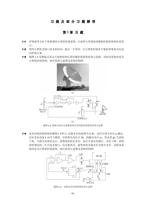
计算机控制系统习题及部分解答
g0=(1/T)*5*abs(1/(10+(GW+ws)*i)); G11=[g0];
g0=(1/T)*5*abs(1/(10+(GW-ws)*i)); G12=[g0];
g0=(1/T)*5*abs(1/(10+(GW+2*ws)*i)); G21=[g0];
g0=(1/T)*5*abs(1/(10+(GW-2*ws)*i)); G22=[g0];
题图 1-6 飞机连续模拟式姿态角控制系统结构示意图
第2章 习 题
2-1 下述信号被理想采样开关采样,采样周期为 T,试写出采样信号的表达式。
(1) f (t) = 1(t)
(2) f (t) = te−at
(3) f (t) = e−at sin(ωt)
解:
∞
∑ (1) f *(t) = 1(kT )δ (t − kT ) ; k =0 ∞
结果表明,不满足采样定理,高频信号将变为低频信号。
2-8
试证明
ZOH
传递函数
Gh
(s)
=
1
−
e− s
sT
中的 s=0 不是 Gh
(s)的极点,而
Y
(
s
)
=
1
− e− s2
sT
中,只有一个单极点 s=0。
证明:
Gh
(s)
=
1
−
e s
−
sT
≈ 1− (1− sT
+ (−sT )2 / 2 + ⋅ ⋅⋅ = T − T 2s + ⋅⋅ ⋅⋅
计算。采样幅频曲线可以用如下 MATLAB 程序绘图:
T=0.1;
数据通信原理实验指导书
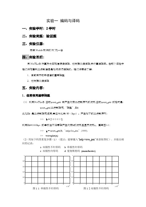
实验一编码与译码一、实验学时:2学时二、实验类型:验证型三、实验仪器:安装Matlab软件的PC机一台四、实验目的:用MATLAB仿真技术实现信源编译码、过失操纵编译码,并计算误码率。
在那个实验中咱们将观看到二进制信息是如何进行编码的。
咱们将要紧了解:1.目前用于数字通信的基带码型2.过失操纵编译码五、实验内容:1.经常使用基带码型(1)利用MATLAB 函数wave_gen 来产生代表二进制序列的波形,函数wave_gen 的格式是:wave_gen(二进制码元,‘码型’,Rb)此处Rb 是二进制码元速度,单位为比特/秒(bps)。
产生如下的二进制序列:>> b = [1 0 1 0 1 1];利用Rb=1000bps 的单极性不归零码产生代表b的波形且显示波形x,填写图1-1:>> x = wave_gen(b,‘unipolar_nrz’,1000);>> waveplot(x)(2)用如下码型重复步骤(1)(提示:能够键入“help wave_gen”来获取帮忙),并做出相应的记录:a 双极性不归零码b 单极性归零码c 双极性归零码d 曼彻斯特码(manchester)x 10-3x 10⁻³图1-1 单极性不归零码图1-2双极性不归零码x 10-3x 10-32.过失操纵编译码(1) 利用MATLAB 函数encode 来对二进制序列进行过失操纵编码, 函数encode 的格式是:A .code = encode(msg,n,k,'linear/fmt',genmat)B .code = encode(msg,n,k,'cyclic/fmt',genpoly)C .code = encode(msg,n,k,'hamming/fmt',prim_poly)其中A .用于产生线性分组码,B .用于产生循环码,C .用于产生hamming 码,msg 为待编码二进制序列,n 为码字长度,k 为分组msg 长度,genmat 为生成矩阵,维数为k*n ,genpoly 为生成多项式,缺省情形下为cyclpoly(n,k)。
gtsam原理
GTSAM原理介绍GTSAM(Generalized Trajectory and Sparse Factor Graphs Optimization)是一个用于非线性优化的开源库,专注于传感器数据处理和SLAM(Simultaneous Localization and Mapping)问题。
它是一个基于因子图的优化框架,可以在不同传感器数据的基础上进行状态估计和地图构建。
为什么选择GTSAMGTSAM的设计目标是提供一个高效、灵活和易于使用的非线性优化框架。
相比于其他优化库,GTSAM具有以下优势: 1. 因子图表示:GTSAM使用因子图来表示问题,将状态变量和约束关系以图的形式表示出来,使得问题更加直观和可理解。
2.稀疏性:GTSAM利用问题的稀疏性,只存储和处理非零元素,大大减少了计算和存储的复杂度。
3. 高效性:GTSAM使用了一些高效的优化算法和数据结构,如QR分解、Cholesky分解等,以提高计算效率。
4. 可扩展性:GTSAM支持自定义因子和变量类型,可以根据具体问题进行扩展和定制。
GTSAM的基本原理GTSAM的基本原理是基于因子图的优化。
因子图是一种用于表示概率模型的图结构,其中节点表示变量,边表示变量之间的关系。
在GTSAM中,因子图由变量节点和因子节点组成,变量节点表示状态变量,因子节点表示约束关系。
变量节点在GTSAM中,变量节点表示状态变量,可以是连续变量、离散变量或者混合变量。
每个变量节点都有一个唯一的ID和一个值。
变量节点的值可以是一个向量、一个矩阵或者其他自定义的数据类型。
因子节点在GTSAM中,因子节点表示约束关系,用于描述传感器测量或其他先验知识。
每个因子节点都有一个唯一的ID和一个因子函数。
因子函数是一个函数,接受一组变量作为输入,并返回一个代价值。
因子函数可以是线性函数、非线性函数或其他自定义的函数。
优化问题在GTSAM中,优化问题可以表示为最小化一个代价函数的问题,代价函数是所有因子函数的加权和。
基于流形学习的高维空间分类器研究的开题报告
基于流形学习的高维空间分类器研究的开题报告1. 研究背景和意义在现实问题中,数据往往具有高维空间特性,并且通常不是线性可分的。
例如,在图像识别和自然语言处理领域,数据往往包含大量的特征。
基于流形学习的高维空间分类器可以有效地处理这些问题,具有广泛的应用价值。
因此,研究基于流形学习的高维空间分类器具有重要的理论和应用意义。
2. 研究内容和方法本研究将从以下三个方面进行探究:①针对高维空间数据分类问题,研究不同的流形学习方法,包括局部线性嵌入(LLE)、加权最近邻(WKNN)和拉普拉斯正则化嵌入(LRE)等方法,比较不同方法的性能。
②研究使用支持向量机(SVM)等传统分类算法和基于流形学习方法的分类器进行对比,并分析其准确性和复杂度。
③在实际应用中,研究如何利用基于流形学习的高维空间分类器解决图像识别和自然语言处理等问题。
3. 研究预期结果预计本研究将得出以下结论:①尽管不同的流形学习方法在处理高维空间数据分类问题方面有所不同,但其性能差异不是很大。
②基于流形学习的高维空间分类器与传统的分类算法相比,在性能和复杂度上具有明显优势。
③基于流形学习的高维空间分类器在图像识别和自然语言处理等领域具有广泛应用前景。
4. 研究计划和进度安排本研究计划如下:第一年:收集和了解基于流形学习的高维空间分类器的相关研究,了解和掌握流形学习和分类器的基本知识和方法,研究局部线性嵌入(LLE)、加权最近邻(WKNN)等流形学习方法。
第二年:进一步研究拉普拉斯正则化嵌入(LRE)等流形学习方法,并将不同方法与传统的分类算法进行对比,比较其准确性和复杂度。
第三年:针对实际应用问题,如图像识别和自然语言处理等,研究如何利用基于流形学习的高维空间分类器解决问题,并进行实验验证。
四年级:撰写论文,准备答辩。
- 1、下载文档前请自行甄别文档内容的完整性,平台不提供额外的编辑、内容补充、找答案等附加服务。
- 2、"仅部分预览"的文档,不可在线预览部分如存在完整性等问题,可反馈申请退款(可完整预览的文档不适用该条件!)。
- 3、如文档侵犯您的权益,请联系客服反馈,我们会尽快为您处理(人工客服工作时间:9:00-18:30)。
Signal Processing71(1998)131—139Generalized gradient vectorflow external forces for active contoursChenyang Xu,Jerry L.Prince *Image Analysis and Communications Laboratory,Department of Electrical and Computer Engineering,The Johns Hopkins Uni v ersity,Baltimore,MD21218,USAAbstractActive contours,or snakes,are used extensively in computer vision and image processing applications,particularly to locate object boundaries.A new type of external force for active contours,called gradient vectorflow(GVF)was introduced recently to address problems associated with initialization and poor convergence to boundary concavities. GVF is computed as a diffusion of the gradient vectors of a gray-level or binary edge map derived from the image.In this paper,we generalize the GVF formulation to include two spatially varying weighting functions.This improves active contour convergence to long,thin boundary indentations,while maintaining other desirable properties of GVF,such as an extended capture range.The original GVF is a special case of this new generalized GVF(GGVF)model.An error analysis for active contour results on simulated test images is also presented. 1998Elsevier Science B.V.All rights reserved.ZusammenfassungAktive Umrisse,oder Schlangen,werden vielfach in Computervision-und Bildverarbeitungs-Anwendungen benutzt, um insbesondere Objektgrenzen zu lokalisieren.Ein neuer Typ a u{erer Kra fte fu r aktive Umrisse,Gradient»ector Flow (GVF)genannt,wurde ku rzlich eingefu hrt,um Probleme anzusprechen,die mit Initialisierung und schlechter Konvergenz zu Grenzkonkavita ten zusammenha ngen.GVF wird als eine Diffusion des Gradientenvektors einer Graustufen-oder ‘Binary Edge’-Karte berechnet,die aus dem Bild gewonnen werden.In diesem Artikel verallgemeinern wir die GVF Formulierung,so da{zwei ra umlich variierende Gewichtsfunktionen eingeschlossen werden.Dies verbessert die Konvergenz aktiver Umrisse zu langen,du nnen Grenzmarkierungen,wa hrend andere wu nschenswerte Eigenschaften des GVF,wie erweiterter Einfangbereich,erhalten bleiben.Das urspru ngliche GVF ist ein Spezialfall dieses neuen verallgemeinerten GVF(GGVF)Modells.Eins Fehleranalyse von Ergebnissen aktiver Umrisse mit simulierten Testbildern wird ebenfalls pra sentiert. 1998Elsevier Science B.V.All rights reserved.Re sumeLes contours actifs,ou serpents(snakes),sont utilise s intensivement en vision par ordinateur et pour les applications de traitement d’images,particulie rement pour localiser les contours d’objects.Un nouveau type de force externe pour les *Corresponding author.Tel.:#14105165192;fax#14105165566;e-mail:prince@.A preliminary version of this paper appeared in the Proceedings of the Johns Hopkins University1997Conference of Information Sciences and Systems.This research was supported by NSF grant MIP9350336.0165-1684/98/$—see front matter 1998Elsevier Science B.V.All rights reserved.PII:S0165-1684(98)00140-6contours actifs,appeleflux de vecteurs gradients(FVG)a e te introduit re cemment pour traiter les proble mes associe s a l’initialisation et la faible convergence vers des concavite s dans les contours.Le FVG est calcule comme une diffusion des vecteurs gradients d’une carte des contours d’une image en niveaux de gris ou binaire.Dans cet article,nous ge ne ralisons la formulation du FVG pour y inclure deux fonctions de poids a variation spatiale.Ceci ame liore la convergence des contours actifs vers les indentations de contoursfines et longues,tout en maintenant les autres proprie te s inte ressantes des FVG comme la plage de capture e tendue.Les FVG originaux sont un cas particulier des mode les de FVG ge ne ralise s.Une analyse de l’erreur des re sultats de contours actifs sur des images de test synthe tiques est aussi pre sente e. 1998Elsevier Science B.V.All rights reserved.Keywords:Edge detection;Image segmentation;Shape representation and recovery;Deformable models;Active contour models;Gradient vectorflow1.IntroductionActive contours,or snakes,are curves defined within an image domain,that can move under the influence of internal forces within the curve itself and external forces derived from the image data[9].The internal and external forces are de-fined so that the snake will conform to an object boundary or other desired features within an image.Snakes are widely used in many applications, including edge detection[9],shape modeling [7,12,13],segmentation[2,6,10]and motion track-ing[10,14].There are two key difficulties in the design and implementation of active contour models.First, the initial contour must,in general,be close to the true boundary or else it will likely converge to the wrong result.Second,active contours have difficulty progressing into boundary concavities[1,5].In [15,16],Xu and Prince developed a new external force,called gradient vectorflow(GVF),which largely solves both problems.GVF is computed as a diffusion of the gradient vectors of a gray-level or binary edge map derived from the image.The resultantfield has a large capture range,which means that the active contour can be initialized far away from the desired boundary.The GVFfield also tends to force active contours into boundary concavities,where traditional snakes have poor convergence.It still has difficulties,however, forcing a snake into long,thin boundary indenta-tions.In this paper,we generalize the GVF formulation to include two spatially varying weighting functions. These weighting functions define a tradeoffbetween smoothness of the resulting GVFfield and its conformity to the gradient of the underlying edge map.The external forcefields derived from this new generalized G»F(GGVF)improve active contour convergence into long,thin boundary indentations, while maintaining other desirable properties of GVF,such as the extended capture range.The original GVF is a special case of GGVF.An error analysis of active contour results on simulated test images is also presented.2.Background2.1.Traditional snakesA traditional snake is a curve x(s)"[x(s),y(s)], s3[0,1],that moves through the spatial domain of an image to minimize the energy functional E" 1( "x (s)" # "x (s)" #E (x(s))d s,(1) where and are weighting parameters that control the snake’s tension and rigidity,respectively,and x (s)and x (s)denote thefirst and second derivatives of x(s)with respect to s.The external energy function E is derived from the image so that it takes on its smaller values at the features of interest,such as boundaries.Examples of typical external energy functions are$G N(x,y)*I(x,y)for lines and !" (G N(x,y)*I(x,y))" for step edges[3,9],where I(x,y)is a gray-level image,G N(x,y)is a two-dimen-sional Gaussian function with standard deviation ,and is the gradient operator.132 C.Xu,J.L.Prince/Signal Processing71(1998)131–139A snake that minimizes E must satisfy the Euler equationx (s)! x(s)! E "0.(2) Tofind a solution to Eq.(2),the snake is made dynamic by treating x as function of time t as well as s—i.e.,x(s,t).Then,the partial derivative of x with respect to t is then set equal to the left-hand side of Eq.(2)as follows:x R(s,t)" x (s,t)! x (s,t)! E .(3) When the solution x(s,t)stabilizes,the term x R(s,t) vanishes and we achieve a solution of Eq.(2).2.2.GVF snakesIn[15,16],we used Eq.(3)as a starting point to define a new snake,called the G»F snake.We proposed to replace the external force term! E in Eq.(3)with a GVFfield (x,y)defined as the equilibrium solution of the following system of partial differential equations:R" !( ! f)" f" ,(4) where R denotes the partial derivative of (x,y,t) with respect to t,and "* /*x #* /*y is the Laplacian operator(applied to each spatial com-ponent of separately).Here f is an edge map derived from the image I(x,y),having the property that it is larger near image edges.This edge map can be either gray-level or binary valued.It can be computed using$G N(x,y)*I(x,y)or " (G N(x,y)*I(x,y))" ,or any conventional image edge detector(cf.[8]).3.Generalized GVFGVF has many desirable properties as an external force for snakes[15,16].It still has difficulties, however,forcing a snake into long,thin boundary indentations.We hypothesized that this difficulty could be caused by excessive smoothing of thefield near the boundaries,governed by the coefficient in Eq.(4).We reasoned that introducing a spatially varying weighting function,instead of the constant ,and decreasing the smoothing effect near strong gradients,could solve this problem.In the following formulation,which we have termed generalized G»F(GGVF),we replace both and" f" in Eq.(4) by more general weighting functions.An alternative generalization,which follows from a variational formulation,is given in Appendix A.We define GGVF as the equilibrium solution of the following vector partial differential equation: R"g(" f") !h(" f")( ! f).(5) Thefirst term on the right is referred to as the smoothing term since this term alone will produce a smoothly varying vectorfield.The second term is referred as the data term since it encourages the vectorfield to be close to f computed from the data.The weighting functions g())and h())apply to the smoothing and data terms,respectively.Since these weighting functions are dependent on the gradient of the edge map which is spatially varying, the weights themselves are spatially varying,in general.Since we want the vectorfield to be slowly varying(or smooth)at locations far from the edges,but to conform to f near the edges,g())and h())should be monotonically non-increasing and non-decreasing functions of" f",respectively. The above equation reduces to that of GVF when g(" f")" ,(6) h(" f")"" f" .(7) Since g())is constant here,smoothing occurs every-where;however,h())grows larger near strong edges, and should dominate at the boundaries.Thus,GVF should provide good edge localization.The effect of smoothing becomes apparent,however,when there are two edges in close proximity,such as when there is a long,thin indentation along the boundary. In this situation,GVF tends to smooth between opposite edges,losing the forces necessary to drive an active contour into this region.To address this problem,weighting functions can be selected such that g())gets smaller as h()) becomes larger.Then,in the proximity of large gradients,there will be very little smoothing,and the effective vectorfield will be nearly equal to theC.Xu,J.L.Prince/Signal Processing71(1998)131—139133gradient of the edge map.There are many ways to specify such pairs of weighting functions.In this paper,we use the following weighting functions for GGVF:g(" f")"e\ D ) ,(8) h(" f")"1!g(" f").(9) The GGVFfield computed using this pair of weight-ing functions will conform to the edge map gradient at strong edges,but will vary smoothly away from the boundaries.The specification of K determines to some extent the degree of tradeoffbetweenfield smoothness and gradient conformity.As in GVF[16],the partial differential equation (5)specifying GGVF,can be implemented using an explicitfinite difference scheme,which is stable if the time step t and the spatial sample intervals x and y satisfyt) x y4g ,where g is the maximum value of g())over the range of gradients encountered in the edge map image.While an implicit scheme for the numerical implementations of Eq.(5)would be uncondi-tionally stable and therefore not need this condition, the explicit scheme is faster.Still faster methods—for example,the multigrid method—are possible.4.Experimental resultsIn the following experiments,all edge maps used in GVF computations were normalized to the range [0,1]in order to remove the dependency on abso-lute image intensity value.The snakes were dynam-ically reparameterized to maintain contour point separation to within0.5—1.5pixels(cf.[11]).The GVF,GGVF and snake parameters are given for each case.A comparison between the performance of the GVF snake and the GGVF snake is shown in ing an edge map obtained from the orig-inal image shown in Fig.1(a),both the GVFfield ( "0.2)and the GGVFfield(K"0.05)were com-puted,as shown zoomed in Fig.1(b)and1(c),respectively.We note that in this experiment boththe GVFfield and the GGVFfield were normalizedwith respect to their magnitudes and used as ex-ternal forces.Next,a snake( "0.25, "0)wasinitialized at the position shown in Fig.1(d)andallowed to converge within each of the externalforcefields.The GVF result,shown in Fig.1(e),stops well short of convergence to the long,thin,boundary indentation.On the other hand,theGGVF result,shown in Fig.1(f),is able to convergecompletely to this same region.It should be notedthat both GVF and GGVF have wide captureranges(which is evident because the initial snake isfairly far away from the object),and they bothpreserve subjective contours(meaning that theycross the short boundary gaps).It turns out that a good result similar to that ofGGVF in Fig.1(f)can be achieved using GVF with "0.01.Because is small in homogeneous regions as well as near the edges,the convergence of GVF isvery slow—it takes an order of magnitude longerthan GGVF or GVF with "0.2.If the GVFiterations are terminated early,then the result hasan undesirably small capture range.This resultshows that GGVF can be thought of as a fasterGVF that preserves boundary detail and has a largecapture range.The GGVF and GVF results willnever be exactly the same,however,since thesmoothing parameter of GGVF goes to zero atedges,an impossibility for GVF.We compared the accuracy of different activecontour formulations using the simple harmoniccurves.These curves were generated according tothe equationr"a#b cos(m #c)by setting a,b,c to suitable values and varying m.Curves corresponding to m"0,2,4,6and8weredigitized on a201;201grid to give the images inFig.2.In order to eliminate the problem of capturerange for traditional active contours so that com-parisons could be made,we initialized the activecontours at the true curves,and let them deformunder the different external forces.After conver-gence,we computed the maximum distance in theradial direction between the true boundary andeach active contour as in[5].To compute themaximum radial error(MRE),all thefinal active134 C.Xu,J.L.Prince/Signal Processing71(1998)131–139Fig.1.(a)A square with a long,thin indentation and broken boundary;(b)original GVF field (zoomed);(c)proposed GGVF field (zoomed);(d)initial snake position for both the GVF snake and the GGVF snake;(e)final result of the GVF snake;and (f)final result of the GGVFsnake.Fig.2.Harmonic curves:r "a #b cos (m #c ).contours were linearly interpolated to maintain a pre-specified small point separation.The max-imum radial errors were measured in terms of pixels.Our experimental results on accuracy are shown in Fig.3.The first three curves shown in this figure resulted from traditional active contour external forces ! E "! (G N (x ,y )*I (x ,y ))for three Gaussian standard deviations ( "1pixel, "3pixels and "6pixels).The fourth curve resulted from the use of the distance potential forces of Cohen and Cohen [4].The last two resulted from GVF ( "0.1)and GGVF (K "0.05).In both cases the test intensity images were used as edge maps.We see that traditional potential forces with small yield small errors.Since the capture range of this type of force is very small,however,larger ’s areC.Xu,J.L.Prince /Signal Processing 71(1998)131—139135Fig.3.Maximum radial error(MRE).often used as thefigure shown,these forces do not yield high accuracy,especially at larger m’s.The distance potential forces,GVF forces and GGVF forces,all yield high accuracy consistently.Distance potential forces,however,have been shown to have poor performance on boundary concavities[16]. We note that thefluctuations of the error curves with increasing m arise due to discretization of the curves on the image grid and to the underlying performance variations of active contours.Active contour algorithms can sometimes be extremely sensitive to noise.To test the noise sensi-tivity of GVF and GGVF,we added impulse noise to the m"8harmonic image in Fig.2.The resulting image is shown in Fig.4(a)with an initial active contour plotted as a circle.The active contour was then allowed to converge,being driven by external forcefields calculated from the noisy image.The results for traditional snakes with "1and "9 are shown in Fig.4(b)and4(c),respectively.The problem with Fig.4(b)is that the snake is simply captured by the local impulsive spikes,rather than the dominantfigure.In Fig.4(c),the large blurs the boundary too much and the snake cannot latch onto the detail.The contour resulting from the distance potential forces is shown in Fig.4(d).Since this external force uses a binary edge map to begin with,it is attracted to the nearest detected edge points,which do not belong to the dominantfigure. The results of GVF and GGVF are shown in Fig.4(e)and4(f),respectively.These results,barely distinguishable from each other,demonstrate a re-markable ability to be both captured from a long distance and to converge extremely well to the dominant shape.It is natural to ask whether there might be a smoothing strategy that would improve the results of the distance potential forces.For example,it may be possible to improve the edge map by prefiltering the image before creating the edge map or by applying a nonlinearfilter to the edge map itself. We have tried several approaches along these lines and have found that it is very difficult to eliminate extraneous boundary points while simultaneously preserving the boundary itself.Another approach is tofilter the distance potential itself in order to136 C.Xu,J.L.Prince/Signal Processing71(1998)131–139Fig.4.(a)Impulse noise corrupted image and the initial snake;(b)and(c)snake results using traditional external forces (G N(x,y)*I(x y)) where "1and9;(d)snake result using distance potential force;(e)GVF snake result with "0.1;and(f)GGVF snake result with K"0.2.The edge map used for both GVF and GGVF snake is f"G N(x,y)*I(x,y),where "1,respectively.All snake results are computed using "0.25and "0.smooth out the energy valleys caused by the ex-traneous edge points.This approachflattens the valley in which the true edge is located and does not eliminate the extraneous valleys,and the converged active contour has poorfidelity to the truth. GVF and GGVF both improve over the distance potential forces by applying a very narrowfilter to the edge map,followed by a vector diffusion that allows the dominant edge map to obliterate the effects of the extraneous edge points scattered throughout the image.It should be noted that if GVF were run with a small parameter,it would not smooth out the extraneous edges.This high-lights an important advantage of GGVF over GVF: that GGVF can support convergence to very thin boundary concavities while simultaneously elimin-ating extraneous edge points.Finally,we compared the qualitative performance of GVF and GGVF active contours on a magnetic resonance image of the left ventricle of a human heart.The original image is shown in Fig.5(a),and its gray-level edge map is shown in Fig.5(b).The goal in this experiment is to extract the boundary description of the inner wall or endocardium of the left ventricle.The initial positions of both GVF and GGVF active contours are shown as circles in gray overlaid on the real images(Fig.5(c)and5(d)).The final contours are shown in white.Many details of the endocardial border are captured by both GVF and GGVF,however,the papillary muscleC.Xu,J.L.Prince/Signal Processing71(1998)131—139137Fig.5.(a)A160;160-pixel magnetic resonance image of the left ventrical of a human heart;(b)the edge map" (G N(x,y)*I(x,y))" with "2.5;(c)the result of GVF snake with "0.1;and(d)the result of GGVF snake with K"0.15.The parameters used for both snakes are "0.1and "0.protruding into the cavity at about the1o’clockposition is represented best by GGVF.In many cases,GGVF and GVF will performvery similarly.Our experiments have revealed cer-tain differences,however,and these may be impor-tant in practice.GGVF will generally show betterconvergence to thin boundary concavities.If the parameter is sufficiently small,however,GVF may achieve similar convergence properties.But inthis case,GVF will require significantly longercomputation time,and noise in the edge map maycause erroneous convergence.In short,GGVF canbe thought of as a computationally faster version ofGVF,with better boundary localization,especially with respect to concave boundaries,and with better noise immunity.5.ConclusionWe have presented a new class of external force models for active contours.It is a generalization of the GVF formulation that includes two spatially varying weighting functions.We showed that GGVF improves active contour convergence into long,thin boundary indentations,and maintains other desirable properties of GVF,such as an extended capture range.We also showed that138 C.Xu,J.L.Prince/Signal Processing71(1998)131–139GGVF has excellent performance on noisy and real medical images.Further investigations into the nature and uses of GGVF are warranted.Also, making connections between GGVF with other applications in image processing and computer vision might provide some new insights or even new solutions to existing problems.Appendix A.Variational framework for generalizing GVFGVF can also be generalized by starting from the variational formulation proposed in[15].Spatially varying weighting functions can be used,leading to the following new variational formulation: " g(" f")" " #h(" f")" ! f" d x d y, where")"is a vector norm and is second-order ing the calculus of variations,we obtain the following Euler equation:)[g(" f") ]!h(" f")( ! f)"0.The solution of this vector equation can be obtained by computing the steady state of the following generalized diffusion equation:R" )[g(" f") ]!h(" f")( ! f),or written more explicitlyR" g(" f")) #g(" f") !h(" f")( ! f). This result is different than GGVF.To under-stand the nature of the difference,we note that if E(" f")) "0,we get GGVF.This condition is data-dependent,however,and is satisfied in homo-geneous regions,but is generally nonzero near the edges.We have implemented this generalized GVF and found that it has very similar properties as GGVF and usually yields a very similar result.This version is more computationally demanding,how-ever.Therefore,despite the aesthetically pleasing property that it satisfies a minimum principle,we advocate GGVF when a generalization to GVF is desired.References[1]A.J.Abrantes,J.S.Marques,A class of constrained cluster-ing algorithms for object boundary extraction,IEEE Trans.Image Process5(November1996)1507—1521.[2]I.Carlbom, D.Terzopoulos,K.M.Harris,Computer-assisted registration,segmentation,and3D reconstruction from images of neuronal tissue sections,IEEE Trans.Med.Imaging13(June1994)351—362.[3]L.D.Cohen,On active contour models and balloons,CVGIP:Image Understanding53(March1991)211—218.[4]L.D.Cohen,I.Cohen,Finite-element methods for activecontour models and balloons for2-D and3-D images, IEEE Trans.Pattern Anal.Machine Intell.15(November 1993)1131—1147.[5]C.Davatzikos,J.L.Prince,An active contour model formapping the cortex,IEEE Trans.Med.Imaging14(March 1995)65—80.[6]R.Durikovic,K.Kaneda,H.Yamashita,Dynamic contour:a texture approach and contour operations,Visual Comput.11(1995)277—289.[7]F.P.Ferrie,garde,P.Whaite,Darboux frames,snakes,and super-quadrics:Geometry from the bottom up,IEEE Trans.Pattern Anal.Machine Intell.15(August1993) 771—784.[8]A.K Jain,Fundamentals of Digital Image Processing,Prentice-Hall,Engelwood Cliffs,NJ,1989.[9]M.Kass,A.Witkin,D.Terzopoulos,Snakes:Active contourmodels,put.Vision.1(4)(1987)321—331.[10]F.Leymarie,M.D.Levine,Tracking deformable objects inthe plane using an active contour model,IEEE Trans.Pattern Anal.Machine Intell.15(6)(1993)617—634. [11]S.Lobregt,M.A.Viergever,A discrete dynamic contourmodel,IEEE Trans.Medical Imaging14(March1995) 12—24.[12]T.McInerney,D.Terzopoulos,A dynamicfinite elementsurface model for segmentation and tracking in multi-diemnsional medical images with application to cardiac 4D image analysis,Comput.Med.Imaging Graph.19(1) (1995)69—83.[13]D.Terzopoulos,K.Fleischer,Deformable models,VisualComput.4(1988)306—331.[14]D.Terzopoulos,R.Szeliski,Tracking with Kalman snakes,in:A.Blake,A.Yuille(Eds.),Artificial Intelligence,MIT Press,Cambridge,MA,1992,pp.3—20.[15]C.Xu,J.L.Prince,Gradient vectorflow:A new externalforce for snakes,IEEE Proc.Conf.on Comput.Vis.Patt.Recog.(CVPR)1997,pp.66—71.[16]C.Xu,J.L.Prince,Snakes,shapes,and gradient vectorflow,IEEE Trans.on Image Process.(March1998)359—369.C.Xu,J.L.Prince/Signal Processing71(1998)131—139139。