1-Point RANSAC for EKF-Based Structure from Motion
田间作物群体三维点云柱体空间分割方法

第37卷第7期农业工程学报V ol.37 No.7 2021年4月Transactions of the Chinese Society of Agricultural Engineering Apr. 2021 175田间作物群体三维点云柱体空间分割方法林承达,韩晶,谢良毅,胡方正(华中农业大学资源与环境学院,武汉430070)摘要:农田作物群体表型信息对于研究作物内部基因改变和培育优良品种具有重要意义。
为实现田间作物群体点云数据中单个植株对象的完整提取与分割,以便于更高效地完成作物个体表型参数的自动测量,该研究提出一种田间作物柱体空间聚类分割方法。
利用三维激光扫描仪获取田间油菜、玉米和棉花的三维点云数据,基于HSI(Hue-Saturation-Intensity,色调、饱和度、亮度)颜色模型进行作物群体目标提取,采用直通滤波方法获取作物茎秆点云,基于茎秆点云数据使用欧氏距离聚类分割算法提取每个植株的聚类中心点,并以聚类中心点建立柱体空间模型,使用该模型分割得到田间作物每个单体植株的点云数据。
试验结果表明,该研究的方法对油菜、玉米和棉花3种作物的分割准确率分别为90.12%、96.63%和100%,与欧氏距离聚类分割结果相比,准确率分别提高了36.42,61.80和82.69个百分点,算法耗时分别缩短为后者的9.98%,16.40%和9.04%,与区域增长算法分割结果相比,该研究的方法可用于不同类型农作物,适用性更强,能够实现农田中较稠密作物植株的分割。
该研究的方法能够实现农田尺度下单个植株的完整提取与分割,具有较高的适用性,可为精确测量作物个体表型信息提供参考。
关键词:作物;激光;三维点云;柱体空间模型;分割doi:10.11975/j.issn.1002-6819.2021.07.021中图分类号:TP391 文献标志码:A 文章编号:1002-6819(2021)-07-0175-08林承达,韩晶,谢良毅,等. 田间作物群体三维点云柱体空间分割方法[J]. 农业工程学报,2021,37(7):175-182. doi:10.11975/j.issn.1002-6819.2021.07.021 Lin Chengda, Han Jing, Xie Liangyi, et al. Cylinder space segmentation method for field crop population using 3D point cloud[J]. Transactions of the Chinese Society of Agricultural Engineering (Transactions of the CSAE), 2021, 37(7): 175-182. (in Chinese with English abstract) doi:10.11975/j.issn.1002-6819.2021.07.021 0 引 言随着人口数量的不断增加,人类对粮食和油料作物的需求急剧上升,但其产量却受到可利用耕地减少、土地荒漠化和自然灾害等的影响而难以提升。
ransac经典文章

PROBLEM: Given the set of seven (x,y) pairs shown in the plot, find a best fit line, assuming that no valid datum deviates from this line by more than 0.8 units.
Communications of the ACM June 1981 Volume 24 Number 6
Fig. 1. Failure of Lowing Out The Worst Residual" Heuristic), to Deal with an Erroneous Data Point.
I. Introduction
(RANSAC),for fitting a model to experimental data is
introduced. RANSAC is capable of interpreting/ smoothing data containing a significant percentage of gross errors, and is thus ideally suited for applications in automated image analysis where interpretation is based on the data provided by error-prone feature detectors. A major portion of this paper describes the application of RANSAC to the Location Determination Problem (LDP): Given an image depicting a set of landmarks with known locations, determine that point in space from which the image was obtained. In response to a RANSAC requirement, new results are derived on the minimum number of landmarks needed to obtain a solution, and algorithms are presented for computing these minimum-landmark solutions in closed form. These results provide the basis for an automatic system that can solve the LDP under difficult viewing
Ransac和圆拟合

课程实验报告
2017 - 2018 学年第一学期
课程名称:计算机视觉及应用
实验名称:
班级:电通1班
学生姓名: 学号: 。
实验日期: 2017.12.1 地点:
指导教师:
成绩评定: 批改日期:
实验数据分析及处理
示例图片RANSAC拟合情况:
通过在MATLAB上仿真,得到RANSAC圆拟合图,如下所示:图1 第一次运行时RANSAC圆拟合图
图2 第二次运行时RANSAC圆拟合图
图3 第三次运行时RANSAC圆拟合图
实验结果分析
1.图1结果分析
如图1所示,随机生成了300个蓝色的点,其中局内点21个,即黄色点,局外点190个,以抽样点为圆心,拟合了一个圆。
2. 图2结果分析
如图2所示,其中局内点11个,局外点200个,得到较好的拟合结果。
3.图3结果分析
如图3所示,其中局内点14个,局外点200个,得到较好的拟合结果。
4.图1、图2、图3横向对比分析
图一、图二、图三,都是经过多次拟合才拟合成功。
可能的原因是样本点是随机产生的,不能确定每次产生的样本点都能成功的拟合。
5.RANSAC拟合原理和流程图
建立模型时利用圆的定义方程:dist(P,A)+dist(P,B)=DIST,其中P为圆上一点,A为圆心。
随机选取三点A,P构建圆模型,计算每个点到此两焦点的距离和与DIST的差值,差值小于一定阈值时的点为符合模型的点,点数最多时的模型即为最佳圆模型,再根据符合条件的点,利用圆一般方程x^2+y^2+Dx+Ey+F=0和得到符合点进行系数拟合,根据函数式画出最终拟合圆。
机器视觉技术中一种基于反对称矩阵及RANSAC算法的摄像机自标定方法

机器视觉技术中一种基于反对称矩阵及RANSAC算法的摄像机自标定方法王赟【摘要】This paper describes a self-calibration method . After establishing fundamental matrix by using matched feature points , six constraints equations was founded from the fundamental matrix based on the character of the skew-symmetric matrix . . Then the intrinsic and ex-trinsic parameters can be determined through the relation of the set of constraints . Ransac method was adopted to exclude the singular points from detected feature points , therefore improve the accuracy of feature matching and camera calibration . Experimental results for real video showed that this method can effectively acquire the intrinsic and extrin-sic parameters , and it can be applied into computer vision field .%介绍了一种摄像机自标定方法,该方法通过匹配的特征点建立标准矩阵后,利用反对称矩阵的性质,将标准矩阵表达式分解成6 个约束方程,通过其约束关系得到摄像机内外参数.同时采用了 RANSAC 算法从检测到的特征点中排除奇异的特征点,对数据集进行筛选,以此提高匹配点的准确度和标定的精度.实验表明该方法能根据真实视频获得摄像机内外参数,能够较好的应用于机器视觉领域.【期刊名称】《现代制造技术与装备》【年(卷),期】2015(000)004【总页数】3页(P92-94)【关键词】摄像机自标定;基本矩阵;反对称矩阵【作者】王赟【作者单位】新乡学院机电工程学院,新乡 453003【正文语种】中文机器视觉技术中一种基于反对称矩阵及RANSAC算法的摄像机自标定方法王赟(新乡学院机电工程学院,新乡453003)摘要:介绍了一种摄像机自标定方法,该方法通过匹配的特征点建立标准矩阵后,利用反对称矩阵的性质,将标准矩阵表达式分解成6个约束方程,通过其约束关系得到摄像机内外参数。
MEWS评分在急诊留观患者护理决策中的作用分析

MEWS评分在急诊留观患者护理决策中的作用分析一、MEWS评分的概念简化急诊患者危重度评估(Modified Early Warning Score,MEWS)是一种通过观察生命体征来评估患者病情变化的评分系统。
MEWS评分包括呼吸频率、心率、收缩压、体温和意识状态五个指标,通过对这些指标进行评分,并将评分结果相加,来评估患者的病情变化程度。
当评分结果高于一定阈值时,就需要及时采取相应的护理措施,以避免患者病情的进一步恶化。
MEWS评分系统简单易行、操作方便,因此在临床中得到了广泛的使用。
二、MEWS评分在急诊留观患者护理决策中的作用1. 及时发现患者病情变化在急诊留观患者的护理过程中,患者病情的变化可能随时发生,而且有些变化可能相当微弱,容易被忽略。
通过对患者进行定期的MEWS评分,可以及时监测患者的生命体征指标,并将评分结果及时记录在案。
一旦发现患者的MEWS评分升高,就可以及时采取护理措施,以防止患者病情的进一步恶化。
MEWS评分在急诊留观患者护理决策中可以起到及时发现患者病情变化的作用。
2. 提高护理质量MEWS评分可以帮助医护人员及时发现患者的病情变化,有利于提高护理质量。
通过对患者进行定期的MEWS评分,可以及时发现患者的病情变化,及时采取相应的护理措施,有利于减少医疗事故的发生,提高医疗质量和护理效果。
3. 促进医护人员间的交流在急诊留观患者的护理决策中,医护人员之间的交流配合是至关重要的。
通过对患者进行定期的MEWS评分,可以使医护人员更好地了解患者的病情变化情况,并及时进行交流,共同制定护理方案,有利于提高医护人员之间的沟通和配合,促进医护团队的协作效率。
三、MEWS评分在急诊留观患者护理决策中的局限性1. 评分标准不够客观MEWS评分系统主要通过对患者的生命体征指标进行评分,存在一定的主观性。
不同的医护人员可能会对患者的生命体征指标进行评判时存在主观性,因此可能会对评分结果产生一定的误差。
基于自然地表的星载光子计数激光雷达在轨标定

第49卷第11期V ol.49N o.ll红外与激光工程Infrared and Laser Engineering2020年11月Nov. 2020基于自然地表的星载光子计数激光雷达在轨标定赵朴凡,马跃,伍煜,余诗哲,李松(武汉大学电子信息学院,湖北武汉430072)摘要:在轨标定技术是影响星载激光雷达光斑定位精度的核心技术之一。
介绍了目前国内外星载 激光雷达的在轨标定技术发展现状,分析了各类在轨标定技术的特点。
针对新型的光子计数模式星载 激光雷达的特性,提出了一种基于自然地表的星载光子计数激光雷达在轨标定新方法,使用仿真点云 对标定算法的正确性进行了验证,并分别使用南极麦克莫多干谷和中国连云港地区的地表数据和美国ICESat-2卫星数据进行了交叉验证实验,实验结果表明:算法标定后的点云相对美国国家航空航天 局提供的官方点云坐标平面偏移在3 m左右,高程偏移在厘米量级。
文中还利用地面人工建筑等特征 点对比了算法标定后的点云与官方点云之间的差异,最后对基于自然地表的在轨标定方法的精度以及 标定场地形的影响进行了讨论。
关键词:光子计数激光雷达;自然地表;在轨标定;卫星激光测高中图分类号:TN958.98 文献标志码:A DOI:10.3788/IRLA20200214Spaceborne photon-counting LiDAR on-orbitcalibration based on natural surfaceZhao Pufan,Ma Yue,Wu Yu,Yu Shizhe,Li Song(School of Electronic Information, Wuhan University, Wuhan 430072, China)Abstract:On-orbit calibration technique is a key factor which affects the photon geolocation accuracy of spaceborne LiDAR. The current status of spaceborne LiDAR on-orbit calibration technique was introduced, and the characteristics of various spaceborne LiDAR on-orbit calibration technique were analyzed. Aiming at the characteristics of the photon counting mode spaceborne LiDAR, a new on-orbit calibration method based on the natural surface was derived, simulated point cloud was used to verify the correctness of the calibration algorithm, and a cross validation experiment was made with the surface data of the Antarctic McMudro Dry Valleys and China Lianyungang areas and ICESat-2 point cloud data, the experimental results show that the plane offset between the point cloud calibrated by proposed algorithm and point cloud provided by National Aeronautics and Space Administration is about 3 m, elevation offset is in centimeter scale. The differences between the point cloud calibrated by the algorithm and the point cloud provided by National Aeronautics and Space Administration were also compared by using the feature points of artificial construction on the ground. Finally, the accuracy of the on- orbit calibration method based on natural surface and the influence of the calibration field topography were discussed.Key words:photon-counting LiDAR; natural surface; on-orbit calibration; spaceborne laser altimetry收稿日期:2020-05-28;修订日期:2020-06-29基金项目:国家自然科学基金(41801261);对地高分国家科技重大专项(11-Y20A12-9001-17/18,42-Y20A11-9001-17/18);中国博士后 科学基金(2016M600612, 20170034)作者简介:赵朴凡(1996-),男,博士生,主要从事激光标定理论与方法方面的研究工作:Email:****************.cn导师简介:李松(1965-),女,教授,博士生导师,博士,主要从事卫星激光遥感技术与设备方面的研究工作Email:**********.cn20200214-1第11期红外与激光工程第49卷0引言星载激光雷达是一种主动式的激光测量设备,它 根据激光脉冲的渡越时间(Time of Flight,ToF)获得 卫星与地表目标间的精确距离值,结合卫星平台的精 确姿态、位置信息以及激光指向信息后可以获得目标 的精确三维坐标。
ABSTRACT Progressive Simplicial Complexes

Progressive Simplicial Complexes Jovan Popovi´c Hugues HoppeCarnegie Mellon University Microsoft ResearchABSTRACTIn this paper,we introduce the progressive simplicial complex(PSC) representation,a new format for storing and transmitting triangu-lated geometric models.Like the earlier progressive mesh(PM) representation,it captures a given model as a coarse base model together with a sequence of refinement transformations that pro-gressively recover detail.The PSC representation makes use of a more general refinement transformation,allowing the given model to be an arbitrary triangulation(e.g.any dimension,non-orientable, non-manifold,non-regular),and the base model to always consist of a single vertex.Indeed,the sequence of refinement transforma-tions encodes both the geometry and the topology of the model in a unified multiresolution framework.The PSC representation retains the advantages of PM’s.It defines a continuous sequence of approx-imating models for runtime level-of-detail control,allows smooth transitions between any pair of models in the sequence,supports progressive transmission,and offers a space-efficient representa-tion.Moreover,by allowing changes to topology,the PSC sequence of approximations achieves betterfidelity than the corresponding PM sequence.We develop an optimization algorithm for constructing PSC representations for graphics surface models,and demonstrate the framework on models that are both geometrically and topologically complex.CR Categories:I.3.5[Computer Graphics]:Computational Geometry and Object Modeling-surfaces and object representations.Additional Keywords:model simplification,level-of-detail representa-tions,multiresolution,progressive transmission,geometry compression.1INTRODUCTIONModeling and3D scanning systems commonly give rise to triangle meshes of high complexity.Such meshes are notoriously difficult to render,store,and transmit.One approach to speed up rendering is to replace a complex mesh by a set of level-of-detail(LOD) approximations;a detailed mesh is used when the object is close to the viewer,and coarser approximations are substituted as the object recedes[6,8].These LOD approximations can be precomputed Work performed while at Microsoft Research.Email:jovan@,hhoppe@Web:/jovan/Web:/hoppe/automatically using mesh simplification methods(e.g.[2,10,14,20,21,22,24,27]).For efficient storage and transmission,meshcompression schemes[7,26]have also been developed.The recently introduced progressive mesh(PM)representa-tion[13]provides a unified solution to these problems.In PM form,an arbitrary mesh M is stored as a coarse base mesh M0together witha sequence of n detail records that indicate how to incrementally re-fine M0into M n=M(see Figure7).Each detail record encodes theinformation associated with a vertex split,an elementary transfor-mation that adds one vertex to the mesh.In addition to defininga continuous sequence of approximations M0M n,the PM rep-resentation supports smooth visual transitions(geomorphs),allowsprogressive transmission,and makes an effective mesh compressionscheme.The PM representation has two restrictions,however.First,it canonly represent meshes:triangulations that correspond to orientable12-dimensional manifolds.Triangulated2models that cannot be rep-resented include1-d manifolds(open and closed curves),higherdimensional polyhedra(e.g.triangulated volumes),non-orientablesurfaces(e.g.M¨o bius strips),non-manifolds(e.g.two cubes joinedalong an edge),and non-regular models(i.e.models of mixed di-mensionality).Second,the expressiveness of the PM vertex splittransformations constrains all meshes M0M n to have the same topological type.Therefore,when M is topologically complex,the simplified base mesh M0may still have numerous triangles(Fig-ure7).In contrast,a number of existing simplification methods allowtopological changes as the model is simplified(Section6).Ourwork is inspired by vertex unification schemes[21,22],whichmerge vertices of the model based on geometric proximity,therebyallowing genus modification and component merging.In this paper,we introduce the progressive simplicial complex(PSC)representation,a generalization of the PM representation thatpermits topological changes.The key element of our approach isthe introduction of a more general refinement transformation,thegeneralized vertex split,that encodes changes to both the geometryand topology of the model.The PSC representation expresses anarbitrary triangulated model M(e.g.any dimension,non-orientable,non-manifold,non-regular)as the result of successive refinementsapplied to a base model M1that always consists of a single vertex (Figure8).Thus both geometric and topological complexity are recovered progressively.Moreover,the PSC representation retains the advantages of PM’s,including continuous LOD,geomorphs, progressive transmission,and model compression.In addition,we develop an optimization algorithm for construct-ing a PSC representation from a given model,as described in Sec-tion4.1The particular parametrization of vertex splits in[13]assumes that mesh triangles are consistently oriented.2Throughout this paper,we use the words“triangulated”and“triangula-tion”in the general dimension-independent sense.Figure 1:Illustration of a simplicial complex K and some of its subsets.2BACKGROUND2.1Concepts from algebraic topologyTo precisely define both triangulated models and their PSC repre-sentations,we find it useful to introduce some elegant abstractions from algebraic topology (e.g.[15,25]).The geometry of a triangulated model is denoted as a tuple (K V )where the abstract simplicial complex K is a combinatorial structure specifying the adjacency of vertices,edges,triangles,etc.,and V is a set of vertex positions specifying the shape of the model in 3.More precisely,an abstract simplicial complex K consists of a set of vertices 1m together with a set of non-empty subsets of the vertices,called the simplices of K ,such that any set consisting of exactly one vertex is a simplex in K ,and every non-empty subset of a simplex in K is also a simplex in K .A simplex containing exactly d +1vertices has dimension d and is called a d -simplex.As illustrated pictorially in Figure 1,the faces of a simplex s ,denoted s ,is the set of non-empty subsets of s .The star of s ,denoted star(s ),is the set of simplices of which s is a face.The children of a d -simplex s are the (d 1)-simplices of s ,and its parents are the (d +1)-simplices of star(s ).A simplex with exactly one parent is said to be a boundary simplex ,and one with no parents a principal simplex .The dimension of K is the maximum dimension of its simplices;K is said to be regular if all its principal simplices have the same dimension.To form a triangulation from K ,identify its vertices 1m with the standard basis vectors 1m ofm.For each simplex s ,let the open simplex smdenote the interior of the convex hull of its vertices:s =m:jmj =1j=1jjsThe topological realization K is defined as K =K =s K s .The geometric realization of K is the image V (K )where V :m 3is the linear map that sends the j -th standard basis vector jm to j 3.Only a restricted set of vertex positions V =1m lead to an embedding of V (K )3,that is,prevent self-intersections.The geometric realization V (K )is often called a simplicial complex or polyhedron ;it is formed by an arbitrary union of points,segments,triangles,tetrahedra,etc.Note that there generally exist many triangulations (K V )for a given polyhedron.(Some of the vertices V may lie in the polyhedron’s interior.)Two sets are said to be homeomorphic (denoted =)if there ex-ists a continuous one-to-one mapping between them.Equivalently,they are said to have the same topological type .The topological realization K is a d-dimensional manifold without boundary if for each vertex j ,star(j )=d .It is a d-dimensional manifold if each star(v )is homeomorphic to either d or d +,where d +=d:10.Two simplices s 1and s 2are d-adjacent if they have a common d -dimensional face.Two d -adjacent (d +1)-simplices s 1and s 2are manifold-adjacent if star(s 1s 2)=d +1.Figure 2:Illustration of the edge collapse transformation and its inverse,the vertex split.Transitive closure of 0-adjacency partitions K into connected com-ponents .Similarly,transitive closure of manifold-adjacency parti-tions K into manifold components .2.2Review of progressive meshesIn the PM representation [13],a mesh with appearance attributes is represented as a tuple M =(K V D S ),where the abstract simpli-cial complex K is restricted to define an orientable 2-dimensional manifold,the vertex positions V =1m determine its ge-ometric realization V (K )in3,D is the set of discrete material attributes d f associated with 2-simplices f K ,and S is the set of scalar attributes s (v f )(e.g.normals,texture coordinates)associated with corners (vertex-face tuples)of K .An initial mesh M =M n is simplified into a coarser base mesh M 0by applying a sequence of n successive edge collapse transforma-tions:(M =M n )ecol n 1ecol 1M 1ecol 0M 0As shown in Figure 2,each ecol unifies the two vertices of an edgea b ,thereby removing one or two triangles.The position of the resulting unified vertex can be arbitrary.Because the edge collapse transformation has an inverse,called the vertex split transformation (Figure 2),the process can be reversed,so that an arbitrary mesh M may be represented as a simple mesh M 0together with a sequence of n vsplit records:M 0vsplit 0M 1vsplit 1vsplit n 1(M n =M )The tuple (M 0vsplit 0vsplit n 1)forms a progressive mesh (PM)representation of M .The PM representation thus captures a continuous sequence of approximations M 0M n that can be quickly traversed for interac-tive level-of-detail control.Moreover,there exists a correspondence between the vertices of any two meshes M c and M f (0c f n )within this sequence,allowing for the construction of smooth vi-sual transitions (geomorphs)between them.A sequence of such geomorphs can be precomputed for smooth runtime LOD.In addi-tion,PM’s support progressive transmission,since the base mesh M 0can be quickly transmitted first,followed the vsplit sequence.Finally,the vsplit records can be encoded concisely,making the PM representation an effective scheme for mesh compression.Topological constraints Because the definitions of ecol and vsplit are such that they preserve the topological type of the mesh (i.e.all K i are homeomorphic),there is a constraint on the min-imum complexity that K 0may achieve.For instance,it is known that the minimal number of vertices for a closed genus g mesh (ori-entable 2-manifold)is (7+(48g +1)12)2if g =2(10if g =2)[16].Also,the presence of boundary components may further constrain the complexity of K 0.Most importantly,K may consist of a number of components,and each is required to appear in the base mesh.For example,the meshes in Figure 7each have 117components.As evident from the figure,the geometry of PM meshes may deteriorate severely as they approach topological lower bound.M 1;100;(1)M 10;511;(7)M 50;4656;(12)M 200;1552277;(28)M 500;3968690;(58)M 2000;14253219;(108)M 5000;029010;(176)M n =34794;0068776;(207)Figure 3:Example of a PSC representation.The image captions indicate the number of principal 012-simplices respectively and the number of connected components (in parenthesis).3PSC REPRESENTATION 3.1Triangulated modelsThe first step towards generalizing PM’s is to let the PSC repre-sentation encode more general triangulated models,instead of just meshes.We denote a triangulated model as a tuple M =(K V D A ).The abstract simplicial complex K is not restricted to 2-manifolds,but may in fact be arbitrary.To represent K in memory,we encode the incidence graph of the simplices using the following linked structures (in C++notation):struct Simplex int dim;//0=vertex,1=edge,2=triangle,...int id;Simplex*children[MAXDIM+1];//[0..dim]List<Simplex*>parents;;To render the model,we draw only the principal simplices ofK ,denoted (K )(i.e.vertices not adjacent to edges,edges not adjacent to triangles,etc.).The discrete attributes D associate amaterial identifier d s with each simplex s(K ).For the sake of simplicity,we avoid explicitly storing surface normals at “corners”(using a set S )as done in [13].Instead we let the material identifier d s contain a smoothing group field [28],and let a normal discontinuity (crease )form between any pair of adjacent triangles with different smoothing groups.Previous vertex unification schemes [21,22]render principal simplices of dimension 0and 1(denoted 01(K ))as points and lines respectively with fixed,device-dependent screen widths.To better approximate the model,we instead define a set A that associates an area a s A with each simplex s 01(K ).We think of a 0-simplex s 00(K )as approximating a sphere with area a s 0,and a 1-simplex s 1=j k 1(K )as approximating a cylinder (with axis (j k ))of area a s 1.To render a simplex s 01(K ),we determine the radius r model of the corresponding sphere or cylinder in modeling space,and project the length r model to obtain the radius r screen in screen pixels.Depending on r screen ,we render the simplex as a polygonal sphere or cylinder with radius r model ,a 2D point or line with thickness 2r screen ,or do not render it at all.This choice based on r screen can be adjusted to mitigate the overhead of introducing polygonal representations of spheres and cylinders.As an example,Figure 3shows an initial model M of 68,776triangles.One of its approximations M 500is a triangulated model with 3968690principal 012-simplices respectively.3.2Level-of-detail sequenceAs in progressive meshes,from a given triangulated model M =M n ,we define a sequence of approximations M i :M 1op 1M 2op 2M n1op n 1M nHere each model M i has exactly i vertices.The simplification op-erator M ivunify iM i +1is the vertex unification transformation,whichmerges two vertices (Section 3.3),and its inverse M igvspl iM i +1is the generalized vertex split transformation (Section 3.4).Thetuple (M 1gvspl 1gvspl n 1)forms a progressive simplicial complex (PSC)representation of M .To construct a PSC representation,we first determine a sequence of vunify transformations simplifying M down to a single vertex,as described in Section 4.After reversing these transformations,we renumber the simplices in the order that they are created,so thateach gvspl i (a i)splits the vertex a i K i into two vertices a i i +1K i +1.As vertices may have different positions in the different models,we denote the position of j in M i as i j .To better approximate a surface model M at lower complexity levels,we initially associate with each (principal)2-simplex s an area a s equal to its triangle area in M .Then,as the model is simplified,wekeep constant the sum of areas a s associated with principal simplices within each manifold component.When2-simplices are eventually reduced to principal1-simplices and0-simplices,their associated areas will provide good estimates of the original component areas.3.3Vertex unification transformationThe transformation vunify(a i b i midp i):M i M i+1takes an arbitrary pair of vertices a i b i K i+1(simplex a i b i need not be present in K i+1)and merges them into a single vertex a i K i. Model M i is created from M i+1by updating each member of the tuple(K V D A)as follows:K:References to b i in all simplices of K are replaced by refer-ences to a i.More precisely,each simplex s in star(b i)K i+1is replaced by simplex(s b i)a i,which we call the ancestor simplex of s.If this ancestor simplex already exists,s is deleted.V:Vertex b is deleted.For simplicity,the position of the re-maining(unified)vertex is set to either the midpoint or is left unchanged.That is,i a=(i+1a+i+1b)2if the boolean parameter midp i is true,or i a=i+1a otherwise.D:Materials are carried through as expected.So,if after the vertex unification an ancestor simplex(s b i)a i K i is a new principal simplex,it receives its material from s K i+1if s is a principal simplex,or else from the single parent s a i K i+1 of s.A:To maintain the initial areas of manifold components,the areasa s of deleted principal simplices are redistributed to manifold-adjacent neighbors.More concretely,the area of each princi-pal d-simplex s deleted during the K update is distributed toa manifold-adjacent d-simplex not in star(a ib i).If no suchneighbor exists and the ancestor of s is a principal simplex,the area a s is distributed to that ancestor simplex.Otherwise,the manifold component(star(a i b i))of s is being squashed be-tween two other manifold components,and a s is discarded. 3.4Generalized vertex split transformation Constructing the PSC representation involves recording the infor-mation necessary to perform the inverse of each vunify i.This inverse is the generalized vertex split gvspl i,which splits a0-simplex a i to introduce an additional0-simplex b i.(As mentioned previously, renumbering of simplices implies b i i+1,so index b i need not be stored explicitly.)Each gvspl i record has the formgvspl i(a i C K i midp i()i C D i C A i)and constructs model M i+1from M i by updating the tuple (K V D A)as follows:K:As illustrated in Figure4,any simplex adjacent to a i in K i can be the vunify result of one of four configurations in K i+1.To construct K i+1,we therefore replace each ancestor simplex s star(a i)in K i by either(1)s,(2)(s a i)i+1,(3)s and(s a i)i+1,or(4)s,(s a i)i+1and s i+1.The choice is determined by a split code associated with s.Thesesplit codes are stored as a code string C Ki ,in which the simplicesstar(a i)are sortedfirst in order of increasing dimension,and then in order of increasing simplex id,as shown in Figure5. V:The new vertex is assigned position i+1i+1=i ai+()i.Theother vertex is given position i+1ai =i ai()i if the boolean pa-rameter midp i is true;otherwise its position remains unchanged.D:The string C Di is used to assign materials d s for each newprincipal simplex.Simplices in C Di ,as well as in C Aibelow,are sorted by simplex dimension and simplex id as in C Ki. A:During reconstruction,we are only interested in the areas a s fors01(K).The string C Ai tracks changes in these areas.Figure4:Effects of split codes on simplices of various dimensions.code string:41422312{}Figure5:Example of split code encoding.3.5PropertiesLevels of detail A graphics application can efficiently transitionbetween models M1M n at runtime by performing a sequence ofvunify or gvspl transformations.Our current research prototype wasnot designed for efficiency;it attains simplification rates of about6000vunify/sec and refinement rates of about5000gvspl/sec.Weexpect that a careful redesign using more efficient data structureswould significantly improve these rates.Geomorphs As in the PM representation,there exists a corre-spondence between the vertices of the models M1M n.Given acoarser model M c and afiner model M f,1c f n,each vertexj K f corresponds to a unique ancestor vertex f c(j)K cfound by recursively traversing the ancestor simplex relations:f c(j)=j j cf c(a j1)j cThis correspondence allows the creation of a smooth visual transi-tion(geomorph)M G()such that M G(1)equals M f and M G(0)looksidentical to M c.The geomorph is defined as the modelM G()=(K f V G()D f A G())in which each vertex position is interpolated between its originalposition in V f and the position of its ancestor in V c:Gj()=()fj+(1)c f c(j)However,we must account for the special rendering of principalsimplices of dimension0and1(Section3.1).For each simplexs01(K f),we interpolate its area usinga G s()=()a f s+(1)a c swhere a c s=0if s01(K c).In addition,we render each simplexs01(K c)01(K f)using area a G s()=(1)a c s.The resultinggeomorph is visually smooth even as principal simplices are intro-duced,removed,or change dimension.The accompanying video demonstrates a sequence of such geomorphs.Progressive transmission As with PM’s,the PSC representa-tion can be progressively transmitted by first sending M 1,followed by the gvspl records.Unlike the base mesh of the PM,M 1always consists of a single vertex,and can therefore be sent in a fixed-size record.The rendering of lower-dimensional simplices as spheres and cylinders helps to quickly convey the overall shape of the model in the early stages of transmission.Model compression Although PSC gvspl are more general than PM vsplit transformations,they offer a surprisingly concise representation of M .Table 1lists the average number of bits re-quired to encode each field of the gvspl records.Using arithmetic coding [30],the vertex id field a i requires log 2i bits,and the boolean parameter midp i requires 0.6–0.9bits for our models.The ()i delta vector is quantized to 16bitsper coordinate (48bits per),and stored as a variable-length field [7,13],requiring about 31bits on average.At first glance,each split code in the code string C K i seems to have 4possible outcomes (except for the split code for 0-simplex a i which has only 2possible outcomes).However,there exist constraints between these split codes.For example,in Figure 5,the code 1for 1-simplex id 1implies that 2-simplex id 1also has code 1.This in turn implies that 1-simplex id 2cannot have code 2.Similarly,code 2for 1-simplex id 3implies a code 2for 2-simplex id 2,which in turn implies that 1-simplex id 4cannot have code 1.These constraints,illustrated in the “scoreboard”of Figure 6,can be summarized using the following two rules:(1)If a simplex has split code c12,all of its parents havesplit code c .(2)If a simplex has split code 3,none of its parents have splitcode 4.As we encode split codes in C K i left to right,we apply these two rules (and their contrapositives)transitively to constrain the possible outcomes for split codes yet to be ing arithmetic coding with uniform outcome probabilities,these constraints reduce the code string length in Figure 6from 15bits to 102bits.In our models,the constraints reduce the code string from 30bits to 14bits on average.The code string is further reduced using a non-uniform probability model.We create an array T [0dim ][015]of encoding tables,indexed by simplex dimension (0..dim)and by the set of possible (constrained)split codes (a 4-bit mask).For each simplex s ,we encode its split code c using the probability distribution found in T [s dim ][s codes mask ].For 2-dimensional models,only 10of the 48tables are non-trivial,and each table contains at most 4probabilities,so the total size of the probability model is small.These encoding tables reduce the code strings to approximately 8bits as shown in Table 1.By comparison,the PM representation requires approximately 5bits for the same information,but of course it disallows topological changes.To provide more intuition for the efficiency of the PSC repre-sentation,we note that capturing the connectivity of an average 2-manifold simplicial complex (n vertices,3n edges,and 2n trian-gles)requires ni =1(log 2i +8)n (log 2n +7)bits with PSC encoding,versus n (12log 2n +95)bits with a traditional one-way incidence graph representation.For improved compression,it would be best to use a hybrid PM +PSC representation,in which the more concise PM vertex split encoding is used when the local neighborhood is an orientableFigure 6:Constraints on the split codes for the simplices in the example of Figure 5.Table 1:Compression results and construction times.Object#verts Space required (bits/n )Trad.Con.n K V D Arepr.time a i C K i midp i (v )i C D i C Ai bits/n hrs.drumset 34,79412.28.20.928.1 4.10.453.9146.1 4.3destroyer 83,79913.38.30.723.1 2.10.347.8154.114.1chandelier 36,62712.47.60.828.6 3.40.853.6143.6 3.6schooner 119,73413.48.60.727.2 2.5 1.353.7148.722.2sandal 4,6289.28.00.733.4 1.50.052.8123.20.4castle 15,08211.0 1.20.630.70.0-43.5-0.5cessna 6,7959.67.60.632.2 2.50.152.6132.10.5harley 28,84711.97.90.930.5 1.40.453.0135.7 3.52-dimensional manifold (this occurs on average 93%of the time in our examples).To compress C D i ,we predict the material for each new principalsimplex sstar(a i )star(b i )K i +1by constructing an ordered set D s of materials found in star(a i )K i .To improve the coding model,the first materials in D s are those of principal simplices in star(s )K i where s is the ancestor of s ;the remainingmaterials in star(a i )K i are appended to D s .The entry in C D i associated with s is the index of its material in D s ,encoded arithmetically.If the material of s is not present in D s ,it is specified explicitly as a global index in D .We encode C A i by specifying the area a s for each new principalsimplex s 01(star(a i )star(b i ))K i +1.To account for this redistribution of area,we identify the principal simplex from which s receives its area by specifying its index in 01(star(a i ))K i .The column labeled in Table 1sums the bits of each field of the gvspl records.Multiplying by the number n of vertices in M gives the total number of bits for the PSC representation of the model (e.g.500KB for the destroyer).By way of compari-son,the next column shows the number of bits per vertex required in a traditional “IndexedFaceSet”representation,with quantization of 16bits per coordinate and arithmetic coding of face materials (3n 16+2n 3log 2n +materials).4PSC CONSTRUCTIONIn this section,we describe a scheme for iteratively choosing pairs of vertices to unify,in order to construct a PSC representation.Our algorithm,a generalization of [13],is time-intensive,seeking high quality approximations.It should be emphasized that many quality metrics are possible.For instance,the quadric error metric recently introduced by Garland and Heckbert [9]provides a different trade-off of execution speed and visual quality.As in [13,20],we first compute a cost E for each candidate vunify transformation,and enter the candidates into a priority queueordered by ascending cost.Then,in each iteration i =n 11,we perform the vunify at the front of the queue and update the costs of affected candidates.4.1Forming set of candidate vertex pairs In principle,we could enter all possible pairs of vertices from M into the priority queue,but this would be prohibitively expensive since simplification would then require at least O(n2log n)time.Instead, we would like to consider only a smaller set of candidate vertex pairs.Naturally,should include the1-simplices of K.Additional pairs should also be included in to allow distinct connected com-ponents of M to merge and to facilitate topological changes.We considered several schemes for forming these additional pairs,in-cluding binning,octrees,and k-closest neighbor graphs,but opted for the Delaunay triangulation because of its adaptability on models containing components at different scales.We compute the Delaunay triangulation of the vertices of M, represented as a3-dimensional simplicial complex K DT.We define the initial set to contain both the1-simplices of K and the subset of1-simplices of K DT that connect vertices in different connected components of K.During the simplification process,we apply each vertex unification performed on M to as well in order to keep consistent the set of candidate pairs.For models in3,star(a i)has constant size in the average case,and the overall simplification algorithm requires O(n log n) time.(In the worst case,it could require O(n2log n)time.)4.2Selecting vertex unifications fromFor each candidate vertex pair(a b),the associated vunify(a b):M i M i+1is assigned the costE=E dist+E disc+E area+E foldAs in[13],thefirst term is E dist=E dist(M i)E dist(M i+1),where E dist(M)measures the geometric accuracy of the approximate model M.Conceptually,E dist(M)approximates the continuous integralMd2(M)where d(M)is the Euclidean distance of the point to the closest point on M.We discretize this integral by defining E dist(M)as the sum of squared distances to M from a dense set of points X sampled from the original model M.We sample X from the set of principal simplices in K—a strategy that generalizes to arbitrary triangulated models.In[13],E disc(M)measures the geometric accuracy of disconti-nuity curves formed by a set of sharp edges in the mesh.For the PSC representation,we generalize the concept of sharp edges to that of sharp simplices in K—a simplex is sharp either if it is a boundary simplex or if two of its parents are principal simplices with different material identifiers.The energy E disc is defined as the sum of squared distances from a set X disc of points sampled from sharp simplices to the discontinuity components from which they were sampled.Minimization of E disc therefore preserves the geom-etry of material boundaries,normal discontinuities(creases),and triangulation boundaries(including boundary curves of a surface and endpoints of a curve).We have found it useful to introduce a term E area that penalizes surface stretching(a more sophisticated version of the regularizing E spring term of[13]).Let A i+1N be the sum of triangle areas in the neighborhood star(a i)star(b i)K i+1,and A i N the sum of triangle areas in star(a i)K i.The mean squared displacement over the neighborhood N due to the change in area can be approx-imated as disp2=12(A i+1NA iN)2.We let E area=X N disp2,where X N is the number of points X projecting in the neighborhood. To prevent model self-intersections,the last term E fold penalizes surface folding.We compute the rotation of each oriented triangle in the neighborhood due to the vertex unification(as in[10,20]).If any rotation exceeds a threshold angle value,we set E fold to a large constant.Unlike[13],we do not optimize over the vertex position i a, but simply evaluate E for i a i+1a i+1b(i+1a+i+1b)2and choose the best one.This speeds up the optimization,improves model compression,and allows us to introduce non-quadratic energy terms like E area.5RESULTSTable1gives quantitative results for the examples in thefigures and in the video.Simplification times for our prototype are measured on an SGI Indigo2Extreme(150MHz R4400).Although these times may appear prohibitive,PSC construction is an off-line task that only needs to be performed once per model.Figure9highlights some of the benefits of the PSC representa-tion.The pearls in the chandelier model are initially disconnected tetrahedra;these tetrahedra merge and collapse into1-d curves in lower-complexity approximations.Similarly,the numerous polyg-onal ropes in the schooner model are simplified into curves which can be rendered as line segments.The straps of the sandal model initially have some thickness;the top and bottom sides of these straps merge in the simplification.Also note the disappearance of the holes on the sandal straps.The castle example demonstrates that the original model need not be a mesh;here M is a1-dimensional non-manifold obtained by extracting edges from an image.6RELATED WORKThere are numerous schemes for representing and simplifying tri-angulations in computer graphics.A common special case is that of subdivided2-manifolds(meshes).Garland and Heckbert[12] provide a recent survey of mesh simplification techniques.Several methods simplify a given model through a sequence of edge col-lapse transformations[10,13,14,20].With the exception of[20], these methods constrain edge collapses to preserve the topological type of the model(e.g.disallow the collapse of a tetrahedron into a triangle).Our work is closely related to several schemes that generalize the notion of edge collapse to that of vertex unification,whereby separate connected components of the model are allowed to merge and triangles may be collapsed into lower dimensional simplices. Rossignac and Borrel[21]overlay a uniform cubical lattice on the object,and merge together vertices that lie in the same cubes. Schaufler and St¨u rzlinger[22]develop a similar scheme in which vertices are merged using a hierarchical clustering algorithm.Lue-bke[18]introduces a scheme for locally adapting the complexity of a scene at runtime using a clustering octree.In these schemes, the approximating models correspond to simplicial complexes that would result from a set of vunify transformations(Section3.3).Our approach differs in that we order the vunify in a carefully optimized sequence.More importantly,we define not only a simplification process,but also a new representation for the model using an en-coding of gvspl=vunify1transformations.Recent,independent work by Schmalstieg and Schaufler[23]de-velops a similar strategy of encoding a model using a sequence of vertex split transformations.Their scheme differs in that it tracks only triangles,and therefore requires regular,2-dimensional trian-gulations.Hence,it does not allow lower-dimensional simplices in the model approximations,and does not generalize to higher dimensions.Some simplification schemes make use of an intermediate vol-umetric representation to allow topological changes to the model. He et al.[11]convert a mesh into a binary inside/outside function discretized on a three-dimensional grid,low-passfilter this function,。
Efficient RANSAC for Point-Cloud Shape Detection
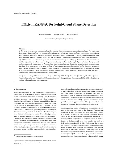
Volume0(1981),Number0pp.1–12Efficient RANSAC for Point-Cloud Shape DetectionRuwen Schnabel Roland Wahl Reinhard Klein†Universität Bonn,Computer Graphics GroupAbstractIn this work we present an automatic algorithm to detect basic shapes in unorganized point clouds.The algorithm decomposes the point cloud into a concise,hybrid structure of inherent shapes and a set of remaining points.Each detected shape serves as a proxy for a set of corresponding points.Our method is based on random sampling and detects planes,spheres,cylinders,cones and tori.For models with surfaces composed of these basic shapes only,e.g.CAD models,we automatically obtain a representation solely consisting of shape proxies.We demonstratethat the algorithm is robust even in the presence of many outliers and a high degree of noise.The proposed method scales well with respect to the size of the input point cloud and the number and size of the shapes within the data.Even point sets with several millions of samples are robustly decomposed within less than a minute.Moreover the algorithm is conceptually simple and easy to implement.Application areas include measurement of physical parameters,scan registration,surface compression,hybrid rendering,shape classification,meshing, simplification,approximation and reverse engineering.Categories and Subject Descriptors(according to ACM CCS):I.4.8[Image Processing and Computer Vision]:Scene AnalysisShape;Surface Fitting;I.3.5[Computer Graphics]:Computational Geometry and Object ModelingCurve, surface,solid,and object representations1.IntroductionDue to the increasing size and complexity of geometric data sets there is an ever-growing demand for concise and mean-ingful abstractions of this data.Especially when dealing with digitized geometry,e.g.acquired with a laser scanner,no handles for modification of the data are available to the user other than the digitized points themselves.However,in or-der to be able to make use of the data effectively,the raw digitized data has to be enriched with abstractions and pos-sibly semantic information,providing the user with higher-level interaction possibilities.Only such handles can pro-vide the interaction required for involved editing processes, such as deleting,moving or resizing certain parts and hence can make the data more readily usable for modeling pur-poses.Of course,traditional reverse engineering approaches can provide some of the abstractions that we seek,but usu-ally reverse engineering focuses onfinding a reconstruction of the underlying geometry and typically involves quite te-dious user interaction.This is not justified in a setting where †e-mail:{schnabel,wahl,rk}@cs.uni-bonn.de a complete and detailed reconstruction is not required at all, or shall take place only after some basic editing operations have been applied to the data.On the other hand,detecting instances of a set of primitive geometric shapes in the point sampled data is a means to quickly derive higher levels of ab-straction.For example in Fig.1patches of primitive shapes provide a coarse approximation of the geometry that could be used to compress the point-cloud very effectively. Another problem arising when dealing with digitized geom-etry is the often huge size of the datasets.Therefore the efficiency of algorithms inferring abstractions of the data is of utmost importance,especially in interactive settings. Thus,in this paper we focus especially onfinding an effi-cient algorithm for point-cloud shape detection,in order to be able to deal even with large point-clouds.Our work is a high performance RANSAC[FB81]algorithm that is capa-ble to extract a variety of different types of primitive shapes, while retaining such favorable properties of the RANSAC paradigm as robustness,generality and simplicity.At the heart of our algorithm are a novel,hierarchically structured sampling strategy for candidate shape generation as well as a novel,lazy cost function evaluation scheme,which signif-c The Eurographics Association and Blackwell Publishing2007.Published by Blackwell Publishing,9600Garsington Road,Oxford OX42DQ,UK and350Main Street,Malden, MA02148,USA.(a)Original(b)ApproximationFigure1:The372detected shapes in the choir screen define a coarse approximation of the surface.icantly reduces overall computational cost.Our method de-tects planes,spheres,cylinders,cones and tori,but additional primitives are possible.The goal of our algorithm is to reli-ably extract these shapes from the data,even under adverse conditions such as heavy noise.As has been indicated above,our method is especially well suited in situations where geometric data is automatically acquired and users refrain from applying surface reconstruc-tion methods,either due to the data’s low quality or due to processing time constraints.Such constraints are typical for areas where high level model interaction is required,as is the case when measuring physical parameters or in interactive, semi-automatic segmentation and postprocessing.Further applications are,for instance,registering many scans of an object,where detecting corresponding primitive shapes in multiple scans can provide good initial matches.High compression rates for point clouds can be achieved if prim-itive shapes are used to represent a large number of points with a small set of parameters.Other areas that can benefit from primitive shape information include hybrid rendering and shape classification.Additionally,a fast shape extraction method as ours can serve as building block in applications such as meshing,simplification,approximation and reverse engineering and bears the potential of significant speed up.2.Previous workThe detection of primitive shapes is a common problem en-countered in many areas of geometry related computer sci-ence.Over the years a vast number of methods have been proposed which cannot all be discussed here in depth.In-stead,here we give a short overview of some of the most important algorithms developed in the differentfields.We treat the previous work on RANSAC algorithms separately in section2.1as it is of special relevance to our work. Vision In computer vision,the two most widely known methodologies for shape extraction are the RANSAC paradigm[FB81]and the Hough transform[Hou62].Both have been proven to successfully detect shapes in2D as well as3D.RANSAC and the Hough transform are reliable even in the presence of a high proportion of outliers,but lack of efficiency or high memory consumption remains their ma-jor drawback[IK88].For both schemes,many acceleration techniques have been proposed,but no one on its own,or combinations thereof,have been shown to be able to provide an algorithm as efficient as ours for the3D primitive shape extraction problem.The Hough transform maps,for a given type of parameter-ized primitive,every point in the data to a manifold in the pa-rameter space.The manifold describes all possible variants of the primitive that contain the original point,i.e.in practice each point casts votes for many cells in a discretized param-eter space.Shapes are extracted by selecting those parame-ter vectors that have received a significant amount of votes. If the parameter space is discretized naively using a simple grid,the memory requirements quickly become prohibitive even for primitives with a moderate number of parameters, such as,for instance,cones.Although several methods have been suggested to alleviate this problem[IK87][XO93]its major application area remains the2D domain where the number of parameters typically is quite small.A notable ex-ception is[VGSR04]where the Hough transform is used to detect planes in3D datasets,as3D planes still have only a small number of parameters.They also propose a two-step procedure for the Hough based detection of cylinders that uses estimated normals in the data points.In the vision community many approaches have been pro-posed for segmentation of range images with primitive shapes.When working on range images these algorithms usually efficiently exploit the implicitly given connectiv-ity information of the image grid in some kind of region growing or region merging step[FEF97][GBS03].This is a fundamental difference to our case,where we are given only an unstructured cloud of points that lacks any explicit connectivity information.In[LGB95]and[LJS97]shapes are found by concurrently growing different seed primi-tives from which a suitable subset is selected according to an MDL criterion(coined the recover-and-select paradigm). [GBS03]detect shapes using a genetic algorithm to optimize a robust MSACfitness function(see also sec.2.1).[MLM01]c The Eurographics Association and Blackwell Publishing2007.introduce involved non-linearfitting functions for primitive shapes that are able to handle geometric degeneracy in the context of recover-and-select segmentation.Another robust method frequently employed in the vision community is the tensor voting framework[MLT00]which has been applied to successfully reconstruct surface geome-try from extremely cluttered scenes.While tensor voting can compete with RANSAC in terms of robustness,it is,how-ever,inherently model-free and therefore cannot be applied to the detection of predefined types of primitive shapes. Reverse engineering In reverse engineering,surface re-covery techniques are usually based on either a separate seg-mentation step or on a variety of region growing algorithms [VMC97][SB95][BGV∗02].Most methods call for some kind of connectivity information and are not well equipped to deal with a large amount of outliers[VMC97].Also these approaches try tofind a shape proxy for every part of the pro-cessed surface with the intent of loading the reconstructed geometry information into a CAD application.[BMV01]de-scribe a system which reconstructs a boundary representa-tion that can be imported into a CAD application from an unorganized point-cloud.However,their method is based on finding a triangulation for the point-set,whereas the method presented in this work is able to operate directly on the input points.This is advantageous as computing a suitable tessela-tion may be extremely costly and becomes very intricate or even ill-defined when there is heavy noise in the data.We do not,however,intend to present a method implementing all stages of a typical reverse engineering process.Graphics In computer graphics,[CSAD04]have recently proposed a general variational framework for approximation of surfaces by planes,which was extended to a set of more elaborate shape proxies by[WK05].Their aim is not only to extract certain shapes in the data,but tofind a globally optimal representation of the object by a given number of primitives.However,these methods require connectivity in-formation and are,due to their exclusive use of least squares fitting,susceptible to errors induced by outliers.Also,the optimization procedure is computationally expensive,which makes the method less suitable for large data sets.The out-put of our algorithm,however,could be used to initialize the set of shape proxies used by these methods,potentially accelerating the convergence of the optimization procedure. While the Hough transform and the RANSAC paradigm have been mainly used in computer vision some applica-tions have also been proposed in the computer graphics com-munity.[DDSD03]employ the Hough transform to identify planes for billboard clouds for triangle data.They propose an extension of the standard Hough transform to include a compactness criterion,but due to the high computational de-mand of the Hough transform,the method exhibits poor run-time performance on large or complex geometry.[WGK05] proposed a RANSAC-based plane detection method for hy-brid rendering of point clouds.To facilitate an efficient plane detection,planes are detected only in the cells of a hier-archical space decomposition and therefore what is essen-tially one plane on the surface is approximated by several planar patches.While this is acceptable for their hybrid ren-dering technique,our methodfinds maximal surface patches in order to yield a more concise representation of the ob-ject.Moreover,higher order primitives are not considered in their approach.[GG04]detect so-called slippable shapes which is a superset of the shapes recognized by our method. They use the eigenvalues of a symmetric matrix derived from the points and their normals to determine the slippability of a point-set.Their detection is a bottom-up approach that merges small initial slippable surfaces to obtain a global de-composition of the model.However the computation of the eigenvalues is costly for large models,the method is sen-sitive to noise and it is hard to determine the correct size of the initial surface patches.A related approach is taken by [HOP∗05].They also use the eigenvalues of a matrix derived from line element geometry to classify surfaces.A RANSAC based segmentation algorithm is employed to detect several shapes in a point-cloud.The method is aimed mainly at mod-els containing small numbers of points and shapes as no opti-mizations or extensions to the general RANSAC framework are adopted.2.1.RANSACThe RANSAC paradigm extracts shapes by randomly draw-ing minimal sets from the point data and constructing cor-responding shape primitives.A minimal set is the smallest number of points required to uniquely define a given type of geometric primitive.The resulting candidate shapes are tested against all points in the data to determine how many of the points are well approximated by the primitive(called the score of the shape).After a given number of trials,the shape which approximates the most points is extracted and the algorithm continues on the remaining data.RANSAC ex-hibits the following,desirable properties:•It is conceptually simple,which makes it easily extensible and straightforward to implement•It is very general,allowing its application in a wide range of settings•It can robustly deal with data containing more than50% of outliers[RL93]Its major deficiency is the considerable computational de-mand if no further optimizations are applied.[BF81]apply RANSAC to extract cylinders from range data,[CG01]use RANSAC and the gaussian image tofind cylinders in3D point clouds.Both methods,though,do not consider a larger number of different classes of shape prim-itives.[RL93]describe an algorithm that uses RANSAC to detect a set of different types of simple shapes.However, their method was adjusted to work in the image domain orc The Eurographics Association and Blackwell Publishing2007.on range images,and they did not provide the optimization necessary for processing large unstructured3D data sets.A vast number of extensions to the general RANSAC scheme have been proposed.Among the more recent ad-vances,methods such as MLESAC[TZ00]or MSAC[TZ98] improve the robustness of RANSAC with a modified score function,but do not provide any enhancement in the perfor-mance of the algorithm,which is the main focus of our work. Nonetheless the integration of a MLESAC scoring function is among the directions of our future work.[Nis05]pro-poses an acceleration technique for the case that the num-ber of candidates isfixed in advance.As it is a fundamen-tal property of our setup that an unknown large number of possibly very small shapes has to be detected in huge point-clouds,the amount of necessary candidates cannot,however, be specified in advance.3.OverviewGiven a point-cloud P={p1,...,p N}with associated nor-mals{n1,...,n N}the output of our algorithm is a set of primitive shapesΨ={ψ1,...,ψn}with corresponding dis-joint sets of points Pψ1⊂P,...,Pψn⊂P and a set of re-maining points R=P\{Pψ1,...,Pψn}.Similar to[RL93]and[DDSD03],we frame the shape extraction problem as an optimization problem defined by a score function.The overall structure of our method is outlined in pseudo-code in algorithm1.In each iteration of the algorithm,the prim-itive with maximal score is searched using the RANSAC paradigm.New shape candidates are generated by randomly sampling minimal subsets of P using our novel sampling strategy(see sec.4.3).Candidates of all considered shape types are generated for every minimal set and all candidates are collected in the set C.Thus no special ordering has to be imposed on the detection of different types of shapes.After new candidates have been generated the one with the high-est score m is computed employing the efficient lazy score evaluation scheme presented in sec.4.5.The best candidate is only accepted if,given the size|m|(in number of points) of the candidate and the number of drawn candidates|C|, the probability P(|m|,|C|)that no better candidate was over-looked during sampling is high enough(see sec.4.2.1).We provide an analysis of our sampling strategy to derive a suit-able probability computation.If a candidate is accepted,the corresponding points P m are removed from P and the can-didates C m generated with points in P m are deleted from C. The algorithm terminates as soon as P(τ,|C|)for a user de-fined minimal shape sizeτis large enough.In our implementation we use a standard score function that counts the number of compatible points for a shape candi-date[RL93][GBS03].The function has two free parame-ters:εspecifies the maximum distance of a compatible point whileαrestricts the deviation of a points’normal from that of the shape.We also ensure that only points forming a con-nected component on the surface are considered(see sec.4.4).Algorithm1Extract shapes in the point cloud PΨ←/0{extracted shapes}C←/0{shape candidates}repeatC←C∪newCandidates(){see sec.4.1and4.3}m←bestCandidate(C){see sec.4.4}if P(|m|,|C|)>p t thenP←P\P m{remove points}Ψ←Ψ∪mC←C\C m{remove invalid candidates}end ifuntil P(τ,|C|)>p treturnΨ4.Our method4.1.Shape estimationAs mentioned above,the shapes we consider in this work are planes,spheres,cylinders,cones and tori which have be-tween three and seven parameters.Every3D-point p i sam-plefixes only one parameter of the shape.In order to reduce the number of required points we compute an approximate surface normal n i for each point[HDD∗92],so that the ori-entation gives us two more parameters per sample.That way it is possible to estimate each of the considered basic shapes from only one or two point samples.However,always using one additional sample is advantageous,because the surplus parameters can be used to immediately verify a candidate and thus eliminate the need of evaluating many relatively low scored shapes[MC02].Plane For a plane,{p1,p2,p3}constitutes a minimal set when not taking into account the normals in the points.To confirm the plausibility of the generated plane,the deviation of the plane’s normal from n1,n2,n3is determined and the candidate plane is accepted only if all deviations are less than the predefined angleα.Sphere A sphere is fully defined by two points with corre-sponding normal vectors.We use the midpoint of the short-est line segment between the two lines given by the points p1and p2and their normals n1and n2to define the center of the sphere c.We take r= p1−c + p2−c2as the sphere ra-dius.The sphere is accepted as a shape candidate only if all three points are within a distance ofεof the sphere and their normals do not deviate by more thanαdegrees.Cylinder To generate a cylinder from two points with nor-mals wefirst establish the direction of the axis with a= n1×n2.Then we project the two parametric lines p1+tn1 and p2+tn2along the axis onto the a·x=0plane and take their intersection as the center c.We set the radius to the dis-tance between c and p1in that plane.Again the cylinder isc The Eurographics Association and Blackwell Publishing2007.verified by applying the thresholds εand αto distance and normal deviation of the samples.Cone Although the cone,too,is fully defined by two points with corresponding normals,for simplicity we use all three points and normals in its generation.To derive the po-sition of the apex c ,we intersect the three planes defined by the point and normal pairs.Then the normal of the plane de-fined by the three points {c +p 1−c p 1−c ,...,c +p 3−c p 3−c }givesthe direction of the axis a .Now the opening angle ωis givenas ω=∑i arccos ((p i −c )·a )3.Afterwards,similar to above,the cone is verified before becoming a candidate shape.Torus Just as in the case of the cone we use one more point than theoretically necessary to ease the computations required for estimation,i.e.four point and normal pairs.The rotational axis of the torus is found as one of the up to two lines intersecting the four point-normal lines p i +λn i [MLM01].To choose between the two possible axes,a full torus is estimated for both choices and the one which causes the smaller error in respect to the four points is selected.To find the minor radius,the points are collected in a plane that is rotated around the axis.Then a circle is computed using three points in this plane.The major radius is given as the distance of the circle center to the plexityThe complexity of RANSAC is dominated by two major fac-tors:The number of minimal sets that are drawn and the cost of evaluating the score for every candidate shape.As we de-sire to extract the shape that achieves the highest possible score,the number of candidates that have to be considered is governed by the probability that the best possible shape is indeed detected,i.e.that a minimal set is drawn that defines this shape.4.2.1.ProbabilitiesConsider a point cloud P of size N and a shape ψtherein consisting of n points.Let k denote the size of a minimal set required to define a shape candidate.If we assume that any k points of the shape will lead to an appropriate candidate shape then the probability of detecting ψin a single pass is:P (n )= n k N k ≈ n N k(1)The probability of a successful detection P (n ,s )after s can-didates have been drawn equals the complementary of s con-secutive failures:P (n ,s )=1−(1−P (n ))s(2)Solving for s tells us the number of candidates T required to detect shapes of size n with a probability P (n ,T )≥p t :T ≥ln (1−p t )ln (1−P (n ))(3)Figure 2:A small cylinder that has been detected by ourmethod.The shape consists of 1066points and was detected among 341,587points.That corresponds to a relative size of 1/3000.For small P (n )the logarithm in the denominator can be approximated by its Taylor series ln (1−P (n ))=−P (n )+O (P (n )2)so that:T ≈−ln (1−p t )P (n )(4)Given the cost C of evaluating the cost function,the asymp-totic complexity of the RANSAC approach is O (TC )=O (1P (n )C ).4.3.Sampling strategyAs can be seen from the last formula,the runtime complexity is directly linked to the success rate of finding good sample sets.Therefore we will now discuss in detail how sampling is performed.4.3.1.Localized samplingSince shapes are local phenomena,the a priori probability that two points belong to the same shape is higher the smaller the distance between the points.In our sampling strategy we want to exploit this fact to increase the probability of draw-ing minimal sets that belong to the same shape.[MTN ∗02]have shown that non-uniform sampling based on locality leads to a significantly increased probability of selecting a set of inliers.From a ball of given radius around an ini-tially unrestrainedly drawn sample the remaining samples are picked to obtain a complete minimal set.This requires to fix a radius in advance,which they derive from a known (or assumed)outlier density and distribution.In our setup however,outlier density and distribution vary strongly for different models and even within in a single model,which renders a fixed radius inadequate.Also,in our case,using minimal sets with small diameter introduces unnecessary stability issues in the shape estimation procedure for shapes that could have been estimated from samples spread farther apart.Therefore we propose a novel sampling strategy that is able to adapt the diameter of the minimal sets to both,outlier density and shape size.cThe Eurographics Association and Blackwell Publishing 2007.We use an octree to establish spatial proximity between sam-ples very efficiently.When choosing points for a new candi-date,we draw thefirst sample p1without restrictions among all points.Then a cell C is randomly chosen from any level of the octree such that p1is contained in C.The k−1other samples are then drawn only from within cell C.The effect of this sampling strategy can be expressed in a new probability P local(n)forfinding a shapeψof size n:P local(n)=P(p1∈ψ)P(p2...p k∈ψ|p2...p k∈C)(5) Thefirst factor evaluates to n/N.The second factor obvi-ously depends on the choice of C.C is well chosen if it con-tains mostly points belonging toψ.The existence of such a cell is backed by the observation that for most points on a shape,except on edges and corners,there exists a neighbor-hood such that all of the points therein belong to that shape. Although in general it is not guaranteed that this neighbor-hood is captured in the cells of the octree,in the case of real-life data,shapes have to be sampled with an adequate density for reliable representation and,as a consequence,for all but very few points such a neighborhood will be at least as large as the smallest cells of the octree.For the sake of analysis,we assume that there exists a C for every p i∈ψsuch thatψwill be supported by half of the points in C, which accounts for up to50%local noise and outliers.We conservatively estimate the probability offinding a good C by1d where d is the depth of the octree(in practice a path of cells starting at the highest good cell to a good leaf will be good as well).The conditional probability for p2,p3∈ψinthe case of a good cell is then described by (|C|/2k−1)(|C|k−1)≈(12)k−1.And substituting yields:P local(n)=nNd2k−1(6)As large shapes can be estimated from large cells(and with high probability this will happen),the stability of the shape estimation is not affected by the sampling strategy.The impact of this sampling strategy is best illustrated with an example.The cylinder depicted in Figure2consists of 1066points.At the time that it belongs to one of the largest shapes in the point-cloud,341,547points of the original2 million still remain.Thus,it then comprises only three thou-sandth of the point-cloud.If an ordinary uniform sampling strategy were to be applied,151,522,829candidates would have to be drawn to achieve a detection probability of99%. With our strategy only64,929candidates have to be gen-erated for the same probability.That is an improvement by three orders of magnitude,i.e.in this case that is the differ-ence between hours and seconds.4.3.1.1.Level weighting Choosing C from a proper level is an important aspect of our sampling scheme.Therefore we can further improve the sampling efficiency by choosing C from a level according to a non-uniform distribution that re-flects the likelihood of the respective level to contain a good cell.To this end,the probability P l of choosing C from level l isfirst initialized with1d.Then for every level l,we keep track of the sumσl of the scores achieved by the candidates generated from a cell on level l.After a given number of candidates has been tested,a new distribution for the levels is computed.The new probabilityˆP l of the level l is given asˆPl=xσlwP l+(1−x)1d,(7)where w=∑d i=1σPi.We set x=.9to ensure that at all times at least10%of the samples are spread uniformly over the levels to be able to detect when new levels start to become of greater importance as more and more points are removed from P.4.3.2.Number of candidatesIn section4.2we gave a formula for the number of candi-dates necessary to detect a shape of size n with a given prob-ability.However,in our case,the size n of the largest shape is not known in advance.Moreover,if the largest candidate has been generated early in the process we should be able to de-tect this lucky case and extract the shape well before achiev-ing a precomputed number of candidates while on the other hand we should use additional candidates if it is still unsure that indeed the best candidate has been detected.Therefore, instead offixing the number of candidates,we repeatedly an-alyze small numbers t of additional candidates and consider the best oneψm generated so far each time.As we want to achieve a low probability that a shape is extracted which is not the real maximum,we observe the probability P(|ψm|,s) with which we would have found another shape of the same size asψm.Once this probability is higher than a threshold p t(we use99%)we conclude that there is a low chance that we have overlooked a better candidate and extractψm.The algorithm terminates as soon as P(τ,s)>p t.4.4.ScoreThe score functionσP is responsible for measuring the qual-ity of a given shape candidate.We use the following aspects in our scoring function:•To measure the support of a candidate,we use the number of points that fall within anε-band around the shape.•To ensure that the points inside the band roughly follow the curvature pattern of the given primitive,we only count those points inside the band whose normals do not deviate from the normal of the shape more than a given angleα.•Additionally we incorporate a connectivity measure: Among the points that fulfill the previous two conditions, only those are considered that constitute the largest con-nected component on the shape.c The Eurographics Association and Blackwell Publishing2007.。
- 1、下载文档前请自行甄别文档内容的完整性,平台不提供额外的编辑、内容补充、找答案等附加服务。
- 2、"仅部分预览"的文档,不可在线预览部分如存在完整性等问题,可反馈申请退款(可完整预览的文档不适用该条件!)。
- 3、如文档侵犯您的权益,请联系客服反馈,我们会尽快为您处理(人工客服工作时间:9:00-18:30)。
1-Point RANSAC for EKF-Based Structure from Motion
I. I NTRODUCTION Classical Structure from Motion (SfM) [12] and Bundle Adjustment (BA) [27] techniques have recently been adapted to sequential and real-time processing of long image sequences. Real-time performance has been achieved by performing live optimization over only a limited number frames of the sequence. If these frames are chosen to be ‘keyframes’ sparsely distributed around a working volume, this permits accurate and drift-free room-sized mapping as in [13]. Or in the case we are considering in this paper, choosing a sliding window of the most recently acquired frames permits accurate camera motion estimation for long trajectories (e.g. [16] for a monocular camere generically known as Visual Odometry, and it has also been demonstrated that the trajectory estimates they produce can be combined with loop closure techniques
Javier Civera, Oscar G. Grasa, Andrew J. Davison and J. M. M. Montiel
Abstract— Recently, classical pairwise Structure From Motion (SfM) techniques have been combined with non-linear global optimization (Bundle Adjustment, BA) over a sliding window to recursively provide camera pose and feature location estimation from long image sequences. Normally called Visual Odometry, these algorithms are nowadays able to estimate with impressive accuracy trajectories of hundreds of meters; either from an image sequence (usually stereo) as the only input, or combining visual and propioceptive information from inertial sensors or wheel odometry. This paper has a double objective. First, we aim to illustrate for the first time how similar accuracy and trajectory length can be achieved by filtering-based visual SLAM methods. Specifically, a camera-centered Extended Kalman Filter is used here to process a monocular sequence as the only input, with 6DOF motion estimated. Features are kept live in the filter while visible as the camera explores forward, and are deleted from the state once they go out of view. This permits an increase in the number of tracked features per frame from tens to around a hundred. While improving the accuracy of the estimation, it makes computationally infeasible the exhaustive Branch and Bound search performed by standard JCBB for match outlier rejection. As a second contribution that overcomes this problem, we present here a RANSAC-like algorithm that exploits the probabilistic prediction of the filter. This use of prior information makes it possible to reduce the size of the minimal data subset to instantiate a hypothesis to the minimum possible of 1 point, greatly increasing the efficiency of the outlier rejection stage. Experimental results from real image sequences covering trajectories of hundreds of meters are presented and compared against RTK GPS ground truth. Estimation errors are about 1% of the trajectory for trajectories up to 650 metres.
Javier Civera, Oscar G. Grasa and J. M. M. Montiel are with Instituto de Investigaci´ on e Ingenier´ ıa de Arag´ on (I3A), Universidad de Zaragoza, Spain. {jcivera, oscgg, josemari}@unizar.es Andrew J. Davison is with the Department of Computing, Imperial College, London, UK. ajd@
to construct large but consistent maps (e.g. [26] or [14] with stereo vision). The front-end image processing algorithms in all of the previously mentioned approaches are similar. In a few words, salient features are extracted and correspondences are searched for between a window of currently live frames. Scene structure and camera poses are estimated for the selected live frames via standard SfM methods. Finally, the solution is refined in a Bundle Adjustment optimization step. Sequential 3D motion and structure estimation from a monocular camera has also been tackled using filtering schemes [1], [4], [9] which propagate a probabilistic state estimate. Accurate estimation for large trajectories have only been achieved after the addition of other estimation techniques, like local mapping and loop closing in [8], [10], [20], [22]. The first aim of this paper is to show how filtering algorithms can reach similar accuracy to current Visual Odometry methods. To achieve this, we used the sensorcentered Extended Kalman Filter, introduced first in the context of laser-based SLAM [3]. Contrary to the standard EKF, where estimates are always referred to a world reference frame, the sensor-centered approach represents all feature locations and the camera motion in a reference frame local to the current camera. The typical correlated feature-sensor uncertainty arising from the uncertain camera location is transferred into uncertainty in the world reference frame, resulting in lower variances for the camera and map features, and thus in smaller linearization errors. Another key difference of our approach when compared against usual EKF visual SLAM is the number of measured features, which we increase from tens to more than a hundred (see figure 1). It has been observed experimentally that this increase highly improves the accuracy of the estimation and also makes scale drift, previously reported in [4], [8], [20], almost vanish for the trajectory lengths considered. The second contribution of this paper is the proposal of a new RANSAC algorithm that exploits the probabilistic prediction obtained from the EKF in order to increase the efficiency of the spurious match rejection step. This need for an increase in the efficiency is motivated by the high computational cost of the Joint Compatibility Branch and Bound algorithm (JCBB) [17], which specifically is exponential in the number of measurements. Although its use has been proven feasible and advisable in [8] for one or two tens of matches, the algorithm quickly becomes computationally intractable when the number of matches grows near a hundred. In recent years, an important stream of research has