运筹学 数据模型与决策教材习题答案
数据模型与决策习题与参考
《数据模型与决议》复习题及参照答案第一章绪言一、填空题1.运筹学的主要研究对象是各样有组织系统的管理问题,经营活动。
2.运筹学的核心是运用数学方法研究各样系统的优化门路及方案,为决议者提供科学决议的依照。
3.模型是一件实质事物或现真相况的代表或抽象。
4、往常对问题中变量值的限制称为拘束条件,它能够表示成一个等式或不等式的会合。
5.运筹学研究和解决问题的基础是最优化技术,并重申系统整体优化功能。
运筹学研究和解决问题的成效拥有连续性。
6.运筹学用系统的看法研究功能之间的关系。
7.运筹学研究和解决问题的优势是应用各学科交错的方法,拥有典型综合应用特征。
8.运筹学的发展趋向是进一步依靠于_计算机的应用和发展。
9.运筹学解决问题时第一要察看待决议问题所处的环境。
10.用运筹学剖析与解决问题,是一个科学决议的过程。
11.运筹学的主要目的在于求得一个合理运用人力、物力和财力的最正确方案。
12.运筹学中所使用的模型是数学模型。
用运筹学解决问题的核心是成立数学模型,并对模型求解。
13用运筹学解决问题时,要剖析,定议待决议的问题。
14.运筹学的系统特色之一是用系统的看法研究功能关系。
15.数学模型中,“s· t ”表示拘束。
16.成立数学模型时,需要回答的问题有性能的客观量度,可控制因素,不行控因素。
17.运筹学的主要研究对象是各样有组织系统的管理问题及经营活动。
二、单项选择题1. 成立数学模型时,考虑能够由决议者控制的因素是( A )A.销售数目B.销售价钱C.顾客的需求D.竞争价钱2.我们能够经过(C)来考证模型最优解。
A.察看B.应用C.实验D.检查3.成立运筹学模型的过程不包含( A )阶段。
A.察看环境B.数据剖析C.模型设计4. 成立模型的一个基本原由是去揭晓那些重要的或相关的(D.模型实行B)A 数目B变量C拘束条件D目标函数5.模型中要求变量取值( D )A可正B可负C非正D非负6. 运筹学研究和解决问题的成效拥有(A)A连续性B整体性C阶段性D重生性7.运筹学运用数学方法剖析与解决问题,以达到系统的最优目标。
《数据模型与决策》复习题及参考答案
《数据模型与决策》复习题及参考答案第一章绪言一、填空题1.运筹学的主要研究对象是各种有组织系统的管理问题,经营活动。
2.运筹学的核心是运用数学方法研究各种系统的优化途径及方案,为决策者提供科学决策的依据。
3.模型是一件实际事物或现实情况的代表或抽象。
4、通常对问题中变量值的限制称为约束条件,它可以表示成一个等式或不等式的集合。
5.运筹学研究和解决问题的基础是最优化技术,并强调系统整体优化功能。
运筹学研究和解决问题的效果具有连续性。
6.运筹学用系统的观点研究功能之间的关系。
7.运筹学研究和解决问题的优势是应用各学科交叉的方法,具有典型综合应用特性。
8.运筹学的发展趋势是进一步依赖于_计算机的应用和发展。
9.运筹学解决问题时首先要观察待决策问题所处的环境。
10.用运筹学分析与解决问题,是一个科学决策的过程。
11.运筹学的主要目的在于求得一个合理运用人力、物力和财力的最佳方案。
12.运筹学中所使用的模型是数学模型。
用运筹学解决问题的核心是建立数学模型,并对模型求解。
13用运筹学解决问题时,要分析,定议待决策的问题。
14.运筹学的系统特征之一是用系统的观点研究功能关系。
15.数学模型中,“s·t”表示约束。
16.建立数学模型时,需要回答的问题有性能的客观量度,可控制因素,不可控因素。
17.运筹学的主要研究对象是各种有组织系统的管理问题及经营活动。
二、单选题1.建立数学模型时,考虑可以由决策者控制的因素是( A )A.销售数量 B.销售价格 C.顾客的需求 D.竞争价格2.我们可以通过( C )来验证模型最优解。
A.观察 B.应用 C.实验 D.调查3.建立运筹学模型的过程不包括( A )阶段。
A.观察环境 B.数据分析 C.模型设计 D.模型实施4.建立模型的一个基本理由是去揭晓那些重要的或有关的( B )A数量 B变量 C 约束条件 D 目标函数5.模型中要求变量取值( D )A可正 B可负 C非正 D非负6.运筹学研究和解决问题的效果具有( A )A 连续性B 整体性C 阶段性D 再生性7.运筹学运用数学方法分析与解决问题,以达到系统的最优目标。
数据、模型与决策(运筹学)课后习题和案例答案009
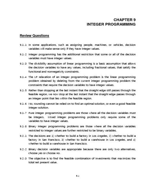
CHAPTER 9INTEGER PROGRAMMING Review Questions9.1-1 In some applications, such as assigning people, machines, or vehicles, decisionvariables will make sense only if they have integer values.9.1-2 Integer programming has the additional restriction that some or all of the decisionvariables must have integer values.9.1-3 The divisibility assumption of linear programming is a basic assumption that allowsthe decision variables to have any values, including fractional values, that satisfy the functional and nonnegativity constraints.9.1-4 The LP relaxation of an integer programming problem is the linear programmingproblem obtained by deleting from the current integer programming problem the constraints that require the decision variables to have integer values.9.1-5 Rather than stopping at the last instant that the straight edge still passes through thefeasible region, we now stop at the last instant that the straight edge passes through an integer point that lies within the feasible region.9.1-6 No, rounding cannot be relied on to find an optimal solution, or even a good feasibleinteger solution.9.1-7 Pure integer programming problems are those where all the decision variables mustbe integers. Mixed integer programming problems only require some of the variables to have integer values.9.1-8 Binary integer programming problems are those where all the decision variablesrestricted to integer values are further restricted to be binary variables.9.2-1 The decisions are 1) whether to build a factory in Los Angeles, 2) whether to build afactory in San Francisco, 3) whether to build a warehouse in Los Angeles, and 4) whether to build a warehouse in San Francisco.9.2-2 Binary decision variables are appropriate because there are only two alternatives,choose yes or choose no.9.2-3 The objective is to find the feasible combination of investments that maximizes thetotal net present value.9.2-4 The mutually exclusive alternatives are to build a warehouse in Los Angeles or build awarehouse in San Francisco. The form of the resulting constraint is that the sum of these variables must be less than or equal to 1 (x3 + x4≤ 1).9.2-5 The contingent decisions are the decisions to build a warehouse. The forms of theseconstraints are x3≤ x1 and x4≤x2.9.2-6 The amount of capital being made available to these investments ($10 million) is amanagerial decision on which sensitivity analysis needs to be performed.9.3-1 A value of 1 is assigned for choosing yes and a value of 0 is assigned for choosing no.9.3-2 Yes-or-no decisions for capital budgeting with fixed investments are whether or notto make a certain fixed investment.9.3-3 Yes-or-no decisions for site selections are whether or not a certain site should beselected for the location of a certain new facility.9.3-4 When designing a production and distribution network, yes-or-no decisions likeshould a certain plant remain open, should a certain site be selected for a new plant, should a certain distribution center remain open, should a certain site be selected fora new distribution center, and should a certain distribution center be assigned toserve a certain market area might arise.9.3-5 Should a certain route be selected for one of the trucks.9.3-6 It is estimated that China is saving about $6.4 billion over the 15 years.9.3-7 The form of each yes-or-no decision is should a certain asset be sold in a certaintime period.9.3-8 The airline industry uses BIP for fleet assignment problems and crew schedulingproblems.9.4-1 A binary decision variable is a binary variable that represents a yes-or-no decision.An auxiliary binary variable is an additional binary variable that is introduced into the model, not to represent a yes-or-no decision, but simply to help formulate the model as a BIP problem.9.4-2 The net profit is no longer directly proportional to the number of units produced so alinear programming formulation is no longer valid.9.4-3 An auxiliary binary variable can be introduced for a setup cost and can be defined as1 if the setup is performed to initiate the production of a certain product and 0 if thesetup is not performed.9.4-4 Mutually exclusive products exist when at most one product can be chosen forproduction due to competition for the same customers.9.4-5 An auxiliary binary variable can be defined as 1 if the product can be produced and 0if the product cannot be produced.9.4-6 An either-or constraint arises because the products are to be produced at eitherPlant 3 or Plant 4, not both.9.4-7 An auxiliary binary variable can be defined as 1 if the first constraint must hold and 0if the second constraint must hold.9.5-1 Restriction 1 is similar to the restriction imposed in Variation 2 except that it involvesmore products and choices.9.5-2 The constraint y1+ y2+ y3≤ 2 forces choosing at most two of the possible newproducts.9.5-3 It is not possible to write a legitimate objective function because profit is notproportional to the number of TV spots allocated to that product.9.5-4 The groups of mutually exclusive alternative in Example 2 are x1 = 0, 1, 2, or 3, x2 = 0,1, 2, or 3, and x3 = 0,1,2, or 3.9.5-5 The mathematical form of the constraint is x1 + x4 + x7 + x10≥ 1. This constraint saysthat sequence 1, 4, 7, and 10 include a necessary flight and that one of the sequences must be chosen to ensure that a crew covers the flight.Problems9.1 a) Let T= the number of tow bars to produceS= the number of stabilizer bars to produce Maximize Profit = $130T+ $150Ssubject to 3.2T+ 2.4S≤ 16 hours2T+ 3S≤15 hours and T≥ 0, S≥ 0 T, S are integers.b) Optimal solution: (T,S) = (0,5). Profit = $750.c)1 2 3 4 5 6 7 8 9A B C D E FTow Bars Stabilizer BarsUnit P rofit$130$150Hours HoursUsed Available M achine 1 3.2 2.412<=16 M achine 22315<=15Tow Bars Stabilizer Bars Total P rofit Units P roduced05$750Hours Used P er Unit P roduced9.2 a)1 2 3 4 5 6 7 8 9 10 11 12 13A B C D E FM odel A M odel B(high speed)(low er speed)Unit Cost$6,000$4,000Total CapacityCapacity Needed Capacity20,00010,00080,000>=75,000 M odel A M odel B(high speed)(low er speed)Total Total Cost P urchase246$28,000 >=>=1M in Needed6Copies per Dayb) Let A= the number of Model A (high-speed) copiers to buyB= the number of Model B (lower-speed) copiers to buy Minimize Cost = $6,000A+ $4,000Bsubject to A+ B≥ 6 copiersA≥ 1 copier20,000A+ 10,000B≥ 75,000 copies/day and A≥ 0, B≥ 0 A, B are integers.c) Optimal solution: (A,B) = (2,4). Cost = $28,000.9.3 a) Optimal solution: (x1, x2) = (2, 3). Profit = 13.b) The optimal solution to the LP-relaxation is (x1, x2) = (2.6, 1.6). Profit = 14.6.Rounded to the nearest integer, (x1, x2) = (3, 2). This is not feasible since it violatesthe third constraint.RoundedFeasible? Constraint Violated PSolution(3,2) No 3rd-(3,1) No 2nd & 3rd-(2,2) Yes - 12(2,1) Yes - 11None of these is optimal for the integer programming model. Two are notfeasible and the other two have lower values of Profit.9.4 a) Optimal solution: (x1, x2) = (2, 3). Profit = 680.b) The optimal solution to the LP-relaxation is (x1, x2) = (2.67, 1.33). Profit = 693.33.Rounded to the nearest integer, (x1, x2) = (3, 1). This is not feasible since it violatesthe second and third constraint.Rounded Solution Feasible? Constraint Violated P(3,1) No 2nd & 3rd-(3,2) No 2nd-(2,2) Yes - 600(2,1) Yes - 520None of these is optimal for the integer programming model. Two are notfeasible and the other two have lower values of Profit.9.5 a)1 2 3 4 5 6 7 8 9 10 11 12A B C D E F GLong-Range M edium-R ange Short-RangeJets Jets JetsAnnual P rofit ($m illion) 4.23 2.3Resource ResourceResource Used P er Unit P roduced Used Available Budget6750351498<=1500M aintenance Capacity 1.667 1.333139.333<=40 P ilot Crew s11130<=30Long-Range M edium-R ange Short-Range Total AnnualJets Jets Jets P rofit ($m illion) P urchase1401695.6b) Let L= the number of long-range jets to purchaseM= the number of medium-range jets to purchaseS= the number of short-range jets to purchase Maximize Annual Profit ($millions) = 4.2L+ 3M+ 2.3Ssubject to 67L+ 50M+ 35S≤ 1,500 ($million)(5/3)L+ (4/3)M+ S≤ 40 (maintenan ce capacity)L+ M+ S≤ 30 (pilot crews) and L≥ 0, M≥ 0, S≥ 0 L, M, S are integers.9.6 a) Let x ij= tons of gravel hauled from pit i to site j(for i= N, S; j= 1, 2, 3)y ij = the number of trucks hauling from pit i to site j (for i = N, S; j = 1, 2, 3) Minimize Cost = $130x N1+ $160x N2+ $150x N3+ $180x S1+ $150x S2+ $160x S3+$50y N1+ $50y N2+ $50y N3+ $50y S1+ $50y S2+ $50y S3 subject to x N1+ x N2+ x N3≤ 18 tons (supply at North Pit)x S1+ x S2+ x S3≤ 14 tons (supply at South Pit)x N1+ x S1= 10 tons (demand at Site 1)x N2+ x S2= 5 tons (demand at Site 2)x N3+ x S3= 10 tons (demand at Site 3)x ij≤ 5y ij(for i= N, S; j= 1, 2, 3) (max 5 tons per truck) and x ij≥ 0, y ij≥ 0, y ij are integers (for i = N, S; j = 1, 2, 3)b)9.7 a) Let F LA= 1 if build a factory in Los Angeles; 0 otherwiseF SF= 1 if build a factory in San Francisco; 0 otherwiseF SD= 1 if build a factory in San Diego; 0 otherwiseW LA= 1 if build a warehouse in Los Angeles; 0 otherwiseW SF= 1 if build a warehouse in San Francisco; 0 otherwiseW SD= 1 if build a warehouse in San Diego; 0 otherwise Maximize NPV ($million) = 9F LA+ 5F SF+ 7F SD+ 6W LA+ 4W SF+ 5W SDsubject to 6F LA+ 3F SF+ 4F SD+ 5W LA+ 2W SF+ 3W SD≤ $10 million (Capital)W LA+ W SF+ W SD≤ 1 warehouseW LA≤ F LA(warehouse only if factory)W SF≤ F SFW SD≤ F SD and F LA, F SF, F SD, W LA, W SF, W SD are binary variables.b)9.8 See the articles in Interfaces.9.9 a) Let E M= 1 if Eve does the marketing; 0 otherwiseE C= 1 if Eve does the cooking; 0 otherwiseE D= 1 if Eve does the dishwashing; 0 otherwiseE L= 1 if Eve does the laundry; 0 otherwiseS M= 1 if Steven does the marketing; 0 otherwiseS C= 1 if Steven does the cooking; 0 otherwiseS D= 1 if Steven does the dishwashing; 0 otherwiseS L= 1 if Steven does the laundry; 0 otherwise Minimize Time (hours) = 4.5E M+ 7.8E C+ 3.6E D+ 2.9E L+4.9S M+ 7.2S C+ 4.3S D+ 3.1S Lsubject to E M+ E C+ E D+ E L= 2 (each person does 2 tasks)S M+ S C+ S D+ S L= 2E M+ S M= 1 (each task is done by 1 person)E C+ S C= 1E D+ S D= 1E L+ S L= 1and E M, E C, E D, E L, S M, S C, S D, S L are binary variables.b)9.10 a) Let x1= 1 if invest in project 1; 0 otherwisex2= 1 if invest in project 2; 0 otherwisex3= 1 if invest in project 3; 0 otherwisex4= 1 if invest in project 4; 0 otherwisex5= 1 if invest in project 5; 0 otherwise Maximize NPV ($million) = 1x1+ 1.8x2+ 1.6x3+ 0.8x4+ 1.4x5subject to 6x1+ 12x2+ 10x3+ 4x4+ 8x5≤ 20 ($million capital available)and x1, x2, x3, x4, x5 are binary variables.b)c)12 13 14 15 16 17 18 19 20 21 22 23A B C D E F G Capital Total Available Undertake?P rofit ($m illion)P roject 1P roject 2P roject 3P roject 4P roject 5($m illion) 10110 3.4 1601010 2.6 1810011 3.2 2010110 3.4 2200111 3.8 24101014 2611001 4.2 2810111 4.8 301101159.11 a)b)18 19 20 21 22 23 24 25 26 27 28 29 30 31 32 33 34A B C D E F G H I Capital Total Available Undertake Investm ent Opportunity?P rofit ($m illion)1234567($m illion) 101000141 80101000032 90011000134 100101000141 110101001045 120101010148 130101011052 140100111056 150101011161 160101011161 170100111165 180100111165 190100111165 2001001111659.12Mutually exclusive alternatives: Each swimmer can only swim one stroke.Each stroke can only be swum by one swimmer.9.139.149.159.16An alternative optimal solution is to produce 3 planes for customer 1 and 2 planes for customer 2.9.179.18 a) Let y ij = 1 if x i = j ; 0 otherwise (for i = 1, 2; and j = 1, 2, 3)Maximize Profit = 3y 11 + 8y 12 + 9y 13 + 9y 21 + 24y 22 + 9y 23 subject to y 11 + y 12 + y 13 ≤ 1 (x i can only take on one value) y 21 + y 22 + y 13 ≤ 1 (y 11 + 2y 12 + 3y 13) + (y 21 + 2y 22 + 3y 23) ≤ 3 andy ij are binary variables (for i = 1, 2; and j = 1, 2, 3)b)c) Optimal Solution (x 1,x 2) = (1, 2). Profit = 27.9.19The constraints in C11:E13 are mutually exclusive alternative (at each stage, exactly one arc is used). The constraints in D6:I8 are contingent decisions (a route can leavea node only if a route enters the node).9.209.21The six equality constraints (total stations = 2; one station assigned to each tract) correspond to mutually exclusive alternatives. In addition, there are the following contingent decision constraints: each tract can only be assigned to a station location if there is a station at that location (D21:D25 ≤ B21:B25; E21:E25 ≤ B21:B25; F21:F25 ≤ B21:B25; G21:G25 ≤ B21:B25; H21:H25 ≤ B21:B25).9.22 a) Let x i= 1 if a station is located in tract i; 0 otherwise (for i= 1, 2, 3, 4, 5)Minimize Cost ($thousand) = 200x1+ 250x2+ 400x3+ 300x4+ 500x5subject to x1+ x3+ x5≥ 1 (stations within 15 minutes of tract 1)x1+ x2+ x4≥ 1 (stations within 15 minutes of tract 2)x2+ x3+ x5≥ 1 (stations within 15 minutes of tract 3)x2+ x3+ x4+ x5≥ 1 (stations within 15 minutes of tract 4)x1+ x3+ x4+ x5≥ 1 (stations within 15 minutes of tract 5) and x i are binary variables (for i = 1, 2, 3, 4, 5).b)Cases9.1 a) With this approach, we need to formulate an integer program for each monthand optimize each month individually.In the first month, Emily does not buy any servers since none of the departmentsimplement the intranet in the first month.In the second month she must buy computers to ensure that the Sales Department can start the intranet. Emily can formulate her decision problem as an integer problem (the servers purchased must be integer. Her objective is to minimize the purchase cost. She has to satisfy to constraints. She cannot spend more than $9500 (she still has her entire budget for the first two months since she didn't buy any computers in the first month) and the computer(s) must support at least 60 employees. She solves her integer programming problem using the Excel solver.5A B C D EUnit Cost=(1-Discount)*OriginalCost=(1-Discount)*OriginalCost=(1-Discount)*OriginalCost=(1-Discount)*OriginalCostRange N ame Cells Budget B8:E8 BudgetAvailable F8 BudgetSpent H8Discount B4:E4 OriginalCost B3:E3 ServersP urchased B12:E12 Support B8:E8 SupportNeeded H8 TotalCost H12 TotalSupport F8 UnitCost B4:E56789101112FTotalSupport=SUM P ROD UCT(Support,ServersP urchased)BudgetSpent=SUM P ROD UCT(B12:E12,ServersP urchased)141516HTotalCost=SUM P ROD UCT(UnitCost,ServersP urchased)Note, that there is a second optimal solution to this integer programming problem. For the same amount of money Emily could buy two standard PC's that would also support 60 employees. However, since Emily knows that she needs to support more employees in the near future, she decides to buy the enhanced PCsince it supports more users.For the third month Emily needs to support 260 users. Since she has already computing power to support 80 users, she now needs to figure out how to support additional 180 users at minimum cost. She can disregard the constraint that the Manufacturing Department needs one of the three larger servers, since she already bought such a server in the previous month. Her task leads her to the following integer programming problem and solution.Emily decides to buy one SGI Workstation in month 3. The network is now able to support 280 users.In the fourth month Emily needs to support a total of 290 users. Since she has already computing power to support 280 users, she now needs to figure out how to support additional 10 users at minimum cost. This task leads her to the following integer programming problem:Emily decides to buy a standard PC in the fourth month. The network is now able to support 310 users.Finally, in the fifth and last month Emily needs to support the entire company witha total of 365 users. Since she has already computing power to support 310 users,she now needs to figure out how to support additional 55 users at minimum cost.This task leads her to the following integer programming problem and solution.Emily decides to buy another enhanced PC in the fifth month. (Note that again she could have also bought two standard PC's, but clearly the enhanced PC provides more room for the workload of the system to grow.) The entire network of CommuniCorp consists now of 1 standard PC, 2 enhanced PC's and 1 SGI workstation and it is able to support 390 users. The total purchase cost for this network is $22,500.b) Due to the budget restriction and discount in the first two months Emily needs todistinguish between the computers she buys in those early months and in the later months. Therefore, Emily uses two variables for each server type.Emily essentially faces four constraints. First, she must support the 60 users in the sales department in the second month. She realizes that, since she no longer buys the computers sequentially after the second month, that it suffices to include only the constraint on the network to support the all users in the entire company. This second constraint requires her to support a total of 365 users. The third constraint requires her to buy at least one of the three large servers. Finally, Emily has to make sure that she stays within her budget during the second month.5A B CMonth 2 Cost=(1-Month2Discount)*Month3to5Cost=(1-Month2Discount)*Month3to5Cost678910111213F Total Support=SUM P R ODUCT(M onth2Support,M onth2P urchases)=SUM P R ODUCT(M onth3to5Support,TotalP urchases)Budget Spent=SUM P R ODUCT(M onth2Budget,M onth2P urchases)171819G HM onth 2 C ost =SU M P R OD U C T(M onth2C ost,M onth2P urchases)M onth 3-5 C ost =SU M P R OD U C T(M onth3to5C ost,M onth3to5P urchases)Total C ost =H 17+H 18Emily should purchase a discounted SGI workstation in the second month, and another regular priced one in the third month. The total purchase cost is $19,000.c) Emily's second method in part (b) finds the cost for the best overall purchase policy. The method in part (a) only finds the best purchase policy for the given month, ignoring the fact that the decision in a particular month has an impact on later decisions. The method in (a) is very short-sighted and thus yields a worse result that the method in part (b).d) Installing the intranet will incur a number of other costs. These costs include:Training cost,Labor cost for network installation,Additional hardware cost for cabling, network interface cards, necessary hubs, etc.,Salary and benefits for a network administrator and web master,Cost for establishing or outsourcing help desk support.e) The intranet and the local area network are complete departures from the waybusiness has been done in the past. The departments may therefore beconcerned that the new technology will eliminate jobs. For example, in the pastthe manufacturing department has produced a greater number of pagers thancustomers have ordered. Fewer employees may be needed when themanufacturing department begins producing only enough pagers to meet orders.The departments may also become territorial about data and procedures, fearingthat another department will encroach on their business. Finally, the departmentsmay be concerned about the security of their data when sending it over thenetwork.9.2 a) We want to maximize the number of pieces displayed in the exhibit. For eachpiece, we therefore need to decide whether or not we should display the piece.Each piece becomes a binary decision variable. The decision variable is assigned1 if we want to display the piece and assigned 0 if we do not want to display thepiece.We group our constraints into four categories – the artistic constraints imposedby Ash, the personal constraints imposed by Ash, the constraints imposed byCeleste, and the cost constraint. We now step through each of these constraintcategories.Artistic Constraints Imposed by AshAsh imposes the following constraints that depend upon the type of art that isdisplayed. The constraints are as follows:1. Ash wants to include only one collage. We have four collages available:“Wasted Resources” by Norm Marson, “Consumerism” by Angie Oldman, “MyNamesake” by Ziggy Lite, and “Narcissism” by Ziggy Lite. A constraint forces us toinclude exactly one of these four pieces (D36=D38 in the spreadsheet model thatfollows).2. Ash wants at least one wire-mesh sculpture displayed if a computer-generated drawing is displayed. We have three wire-mesh sculptures available and two computer-generated drawings available. Thus, if we include either one or two computer-generated drawings, we have to include at least one wire-mesh sculpture. Therefore, we constrain the total number of wire-mesh sculptures (total) to be at least (1/2) time the total number of computer-generated drawings (L40 ≥ N40).3. Ash wants at least one computer-generated drawing displayed if a wire-mesh sculpture is displayed. We have two computer-generated drawings available and three wire-mesh sculptures available. Thus, if we include one, two, or three wire-mesh sculptures, we have to include either one or two computer-generated drawings. Therefore, we constraint the total number of wire-mesh sculptures (total) to be at least (1/3) times the total number of computer-generated drawings (L41 ≥ N41).4. Ash wants at least one photo-realistic painting displayed. We have three photo-realistic paintings available: “Storefront Window” by David Lyman, “Harley” by David Lyman, and “Rick” by Rick Rawls. At least one of these three paintings has to be displayed (G36 ≥ G38).5. Ash wants at least one cubist painting displayed. We have three cubist paintings available: “Rick II” by Rick Rawls, “Study of a Violin” by Helen Row, and “Study of a Fruit Bowl” by Helen Row. At least one of these three paintings has t o be displayed (H36 ≥ H38).6. Ash wants at least one expressionist painting displayed. We have only one expressionist painting available: “Rick III” by Rick Rawls. This painting has to be displayed (I36 ≥ I38).7. Ash wants at least one watercolor painting displayed. We have six watercolor paintings available: “Serenity” by Candy Tate, “Calm Before the Storm” by Candy Tate, “All That Glitters” by Ash Briggs, “The Rock” by Ash Briggs, “Winding Road” by Ash Briggs, and “Dreams Come True” by Ash Br iggs. At least one of these six paintings has to be displayed (J36 ≥ J38).8. Ash wants at least one oil painting displayed. We have five oil paintings available: “Void” by Robert Bayer, “Sun” by Robert Bayer, “Beyond” by Bill Reynolds, “Pioneers” by Bill Reynolds, and “Living Land” by Bear Canton. At least one of these five paintings has to be displayed (K36 ≥ K38).9. Finally, Ash wants the number of paintings to be no greater than twice the number of other art forms. We have 18 paintings available and 16 other art forms available. We classify the followi ng pieces as paintings: “Serenity,” “Calm Before the Storm,” “Void,” “Sun,” “Storefront Window,” “Harley,” “Rick,” “Rick II,” “Rick III,” “Beyond,” “Pioneers,” “Living Land,” “Study of a Violin,” “Study of a Fruit Bowl,” “All That Glitters,” “The Rock,” “Winding Road,” and “Dreams Come True.” The total number of these paintings that we display has to be less than or equal to twice the total number of other art forms we display (L42 ≤ N42).Personal Constraints Imposed by Ash 1. Ash wants all of his own paintings included in the exhibit, so we must include “All That Glitters,” “The Rock,” “Winding Road,” and “Dreams Come True.” (In the spreadsheet model, we constraint the total number of Ash paintings to equal 4: N36=N38.)2. Ash wants all of Candy Tate’s work included in the exhibit, so we must include “Serenity” and “Calm Before the Storm.” (In the spreadsheet model, we constrain the total number of Candy Tate works to equal 2: O36=O38.)3. Ash wants to include at least one piece from David Lyman, so we have to include one or more of the pieces “Storefront Window” and “Harley”(P36 ≥ P38).4. Ash wants to include at least one piece from Rick Rawls, so we have to include one or more of the pieces “Rick,” “Rick II,” and “Rick III” (Q36 ≥ Q38)5. Ash wants to display as many pieces from David Lyman as from Rick Rawls. Therefore we constrain the total number of David Lyman works to equal the total number of Rick Rawls works (L43 = N43).6. Finally, Ash wants at most one piece from Ziggy Lite displayed. We can therefore include no more than one of “My Namesake” and “Narcissism”(R36 ≤ R38).Constraints Imposed by Celeste 1. Celeste wants to include at least one piece from a female artist for every two pieces included from a male artist. We have 11 pieces by female artists available: “Chaos Reigns” by Rita Losky, “Who Has Control?” by Rita Losky, “Domestication” by Rita Losky, “Innocence” by Rita Losky, “Serenity” by Candy Tate, “Calm Before the Storm” by Candy Tate, “Consumerism” by Angie Oldman, “Reflection” by Angie Oldman, “Trojan Victory” by Angie Oldman, “Study of a Violin” by Helen Row, and “Study of a Fruit Bowl” by Helen Row. The total number of these pieces has to be greater-than-or-equal-to (1/2) times the total number of pieces by male artists (L44 ≥ N44).2. Celeste wants at least one of the pieces “Aging Earth” and “Wasted Resources” displayed in order to advance environmentalism (V36 ≥ V38).3. Celeste wants to include at least one piece by Bear Canton, so we must include one or more o f the pieces “Wisdom,” “Superior Powers,” and “Living Land” to advance Native American rights (W36 ≥ W38).4. Celeste wants to include one or more of the pieces “Chaos Reigns,” “Who Has Control,” “Beyond,” and “Pioneers” to advance science (X36 ≥ X38).5. Celeste knows that the museum only has enough floor space for four sculptures. We have six sculptures available: “Perfection” by Colin Zweibell, “Burden” by Colin Zweibell, “The Great Equalizer” by Colin Zweibell, “Aging Earth” by Norm Marson, “Reflection” by Angie Oldman, and “Trojan Victory” by Angie Oldman. We can only include a maximum of four of these six sculptures (Y36 ≤ Y38).6. Celeste also knows that the museum only has enough wall space for 20 paintings, collages, and drawings. We have 28 paintings, collages, and drawings available: “Chaos Reigns,” “Who Has Control,” “Domestication,” “Innocence,” “Wasted Resources,” “Serenity,” “Calm Before the Storm,” “Void,” “Sun,” “Storefront Window,” “Harley,” “Consumerism,” “Rick,” “Rick II,” “Rick III,” “Beyond,” “Pioneers,” “Wisdom,” “Superior Powers,” “Living Land,” “Study of a Violin,” “Study of a Fruit Bowl,” “My Namesake,” “Narcissism,” “All That Glitters,” “The Rock,” “Winding Road,” and “Dreams Come True.” We can only include a maximum of 20 of these 28 wall pieces (Z36 ≤ Z38).7. Finally, Celeste wants “Narcissism” displayed if “Reflection” is displayed. So if the decision variable for “Reflection” is 1, the decision variable for “Narcissism” must also be 1. However, the decision variable for “Narcissism” can still be 1 even if the decision variable for “Reflection” is 0 (L45 ≥ N45).Cost Constraint The cost of all of the pieces displayed has to be less than or equal to $4 million (C36 ≤ C38).。
数据模型与决策(运筹学)课后习题和案例答案(6)
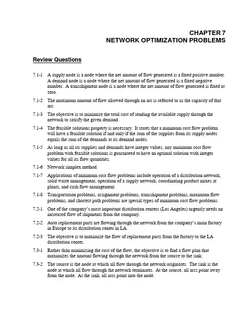
CHAPTER 7NETWORK OPTIMIZATION PROBLEMS Review Questions7.1-1 A supply node is a node where the net amount of flow generated is a fixed positive number.A demand node is a node where the net amount of flow generated is a fixed negativenumber. A transshipment node is a node where the net amount of flow generated is fixed at zero.7.1-2 The maximum amount of flow allowed through an arc is referred to as the capacity of thatarc.7.1-3 The objective is to minimize the total cost of sending the available supply through thenetwork to satisfy the given demand.7.1-4 The feasible solutions property is necessary. It states that a minimum cost flow problemwill have a feasible solution if and only if the sum of the supplies from its supply nodesequals the sum of the demands at its demand nodes.7.1-5 As long as all its supplies and demands have integer values, any minimum cost flowproblem with feasible solutions is guaranteed to have an optimal solution with integervalues for all its flow quantities.7.1-6 Network simplex method.7.1-7 Applications of minimum cost flow problems include operation of a distribution network,solid waste management, operation of a supply network, coordinating product mixes atplants, and cash flow management.7.1-8 Transportation problems, assignment problems, transshipment problems, maximum flowproblems, and shortest path problems are special types of minimum cost flow problems. 7.2-1 One of the company’s most important distribution centers (Los Angeles) urgently needs anincreased flow of shipments from the company.7.2-2 Auto replacement parts are flowing through the network from the company’s main factoryin Europe to its distribution center in LA.7.2-3 The objective is to maximize the flow of replacement parts from the factory to the LAdistribution center.7.3-1 Rather than minimizing the cost of the flow, the objective is to find a flow plan thatmaximizes the amount flowing through the network from the source to the sink.7.3-2 The source is the node at which all flow through the network originates. The sink is thenode at which all flow through the network terminates. At the source, all arcs point awayfrom the node. At the sink, all arcs point into the node.7.3-3 The amount is measured by either the amount leaving the source or the amount entering thesink.7.3-4 1. Whereas supply nodes have fixed supplies and demand nodes have fixed demands, thesource and sink do not.2. Whereas the number of supply nodes and the number of demand nodes in a minimumcost flow problem may be more than one, there can be only one source and only onesink in a standard maximum flow problem.7.3-5 Applications of maximum flow problems include maximizing the flow through adistribution network, maximizing the flow through a supply network, maximizing the flow of oil through a system of pipelines, maximizing the flow of water through a system ofaqueducts, and maximizing the flow of vehicles through a transportation network.7.4-1 The origin is the fire station and the destination is the farm community.7.4-2 Flow can go in either direction between the nodes connected by links as opposed to onlyone direction with an arc.7.4-3 The origin now is the one supply node, with a supply of one. The destination now is theone demand node, with a demand of one.7.4-4 The length of a link can measure distance, cost, or time.7.4-5 Sarah wants to minimize her total cost of purchasing, operating, and maintaining the carsover her four years of college.7.4-6 When “real travel” through a network can end at more that one node, a dummy destinationneeds to be added so that the network will have just a single destination.7.4-7 Quick’s management must consider trade-offs between time and cost in making its finaldecision.7.5-1 The nodes are given, but the links need to be designed.7.5-2 A state-of-the-art fiber-optic network is being designed.7.5-3 A tree is a network that does not have any paths that begin and end at the same nodewithout backtracking. A spanning tree is a tree that provides a path between every pair of nodes. A minimum spanning tree is the spanning tree that minimizes total cost.7.5-4 The number of links in a spanning tree always is one less than the number of nodes.Furthermore, each node is directly connected by a single link to at least one other node. 7.5-5 To design a network so that there is a path between every pair of nodes at the minimumpossible cost.7.5-6 No, it is not a special type of a minimum cost flow problem.7.5-7 A greedy algorithm will solve a minimum spanning tree problem.17.5-8 Applications of minimum spanning tree problems include design of telecommunicationnetworks, design of a lightly used transportation network, design of a network of high- voltage power lines, design of a network of wiring on electrical equipment, and design of a network of pipelines.Problems7.1a)b)c)1[40] 6 S17 4[-30] D1 [-40] D2 [60] 5 8S2 6[-30] D37.2a)supply nodestransshipment nodesdemand nodesb)[200] P1560 [150]425 [125][0] W1505[150]490 [100]470 [100][-150]RO1[-200]RO2P2 [300]c)510 [175]600 [200][0] W2390 [125]410[150] 440[75]RO3[-150]7.3a)supply nodestransshipment nodesdemand nodesV1W1F1V2V3W2 F21P1W1RO1RO2P2W2RO3[-50] SE3000[20][0]BN5700[40][0]HA[50]BE 4000 6300[40][30] [0][0]NY2000[60]2400[20]3400[10] 4200[80][0]5900[60]5400[40]6800[50]RO[0]BO[0]2500[70]2900[50]b)c)7.4a)LA 3100 NO 6100 LI 3200 ST[-130] [70] [30] [40] [130]1[70]11b)c) The total shipping cost is $2,187,000.7.5a)[0][0] 5900RONY[60] 5400[0] 2900 [50]4200 [80][0] [40] 6800 [50]BO[0] 2500LA 3100 NO 6100 LI 3200 ST [-130][70][30] [40][130]b)c)SEBNHABERONYNY(80) [80] (50) [60](30)[40] ROBO (40)(50) [50] (70)[70]11d)e)f) $1,618,000 + $583,000 = $2,201,000 which is higher than the total in Problem 7.5 ($2,187,000). 7.6LA(70) NO[50](30)LI (30) ST[70][30] [40]There are only two arcs into LA, with a combined capacity of 150 (80 + 70). Because ofthis bottleneck, it is not possible to ship any more than 150 from ST to LA. Since 150 actually are being shipped in this solution, it must be optimal. 7.7[-50] SE3000 [20] [0] BN 5700 [40][0] HA[50] BE4000 6300[40][0] NY2000 [60] 2400 [20][30] [0]5900RO [60]17.8 a) SourcesTransshipment Nodes Sinkb)7.9 a)AKR1[75]A [60]R2[65] [40][50][60] [45]D [120] [70]B[55]E[190]T [45][80] [70][70]R3CF[130][90]SE PT KC SL ATCHTXNOMES S F F CAb)Oil Fields Refineries Distribution CentersTXNOPTCACHATAKSEKCME c)SLSFTX[11][7] NO[5][9] PT[8] [2][5] CA [4] [7] [8] [7] [4] [6][8] CH [7][5][9] [4] ATAK [3][6][6][12] SE KC[8][9][4][8] [7] [12] [11]MESL [9]SF[15][7]d)3Shortest path: Fire Station – C – E – F – Farming Community 7.11 a)A70D40 60O60 5010 B 20 C5540 10 T50E801c)Shortest route: Origin – A – B – D – Destinationd)Yese)Yes7.12a)31,00018,000 21,00001238,000 10,000 12,000b)17.13a) Times play the role of distances.B 2 2 G5ACE 1 31 1b)7.14D F1. C---D: Cost = 14.E---G: Cost = 5E---F: Cost = 1 *choose arbitrarilyD---A: Cost = 4 2.E---G: Cost = 5 E---B: Cost = 7 E---B: Cost = 7 F---G: Cost = 7 E---C: Cost = 4 C---A: Cost = 5F---G: Cost = 7C---B: Cost = 2 *lowestF---C: Cost = 3 *lowest5.E---G: Cost = 5 F---D: Cost = 4 D---A: Cost = 43. E---G: Cost = 5 B---A: Cost = 2 *lowestE---B: Cost = 7 F---G: Cost = 7 F---G: Cost = 7 C---A: Cost = 5F---D: Cost = 46.E---G: Cost = 5 *lowestC---D: Cost = 1 *lowestF---G: Cost = 7C---A: Cost = 5C---B: Cost = 2Total = $14 million7.151. B---C: Cost = 1 *lowest 4. B---E: Cost = 72. B---A: Cost = 4 C---F: Cost = 4 *lowestB---E: Cost = 7 C---E: Cost = 5C---A: Cost = 6 D---F: Cost = 5C---D: Cost = 2 *lowest 5. B---E: Cost = 7C---F: Cost = 4 C---E: Cost = 5C---E: Cost = 5 F---E: Cost = 1 *lowest3. B---A: Cost = 4 *lowest F---G: Cost = 8B---E: Cost = 7 6. E---G: Cost = 6 *lowestC---A: Cost = 6 F---G: Cost = 8C---F: Cost = 4C---E: Cost = 5D---A: Cost = 5 Total = $18,000D---F: Cost = 57.16B 34 2E HA D 2 G I K3C F 12J34B41E6A C41G2 FD1. F---G: Cost = 1 *lowest 6. D---A: Cost = 62. F---C: Cost = 6 D---B: Cost = 5F---D: Cost = 5 D---C: Cost = 4F---I: Cost = 2 *lowest E---B: Cost = 3 *lowestF---J: Cost = 5 F---C: Cost = 6G---D: Cost = 2 F---J: Cost = 5G---E: Cost = 2 H---K: Cost = 7G---H: Cost = 2 I---K: Cost = 8G---I: Cost = 5 I---J: Cost = 33. F---C: Cost = 6 7. B---A: Cost = 4F---D: Cost = 5 D---A: Cost = 6F---J: Cost = 5 D---C: Cost = 4G---D: Cost = 2 *lowest F---C: Cost = 6G---E: Cost = 2 F---J: Cost = 5G---H: Cost = 2 H---K: Cost = 7I---H: Cost = 2 I---K: Cost = 8I---K: Cost = 8 I---J: Cost = 3 *lowestI---J: Cost = 3 8. B---A: Cost = 4 *lowest4. D---A: Cost = 6 D---A: Cost = 6D---B: Cost = 5 D---C: Cost = 4D---E: Cost = 2 *lowest F---C: Cost = 6D---C: Cost = 4 H---K: Cost = 7F---C: Cost = 6 I---K: Cost = 8F---J: Cost = 5 J---K: Cost = 4G---E: Cost = 2 9. A---C: Cost = 3 *lowestG---H: Cost = 2 D---C: Cost = 4I---H: Cost = 2 F---C: Cost = 6I---K: Cost = 8 H---K: Cost = 7I---J: Cost = 3 I---K: Cost = 85. D---A: Cost = 6 J---K: Cost = 4D---B: Cost = 5 10. H---K: Cost = 7D---C: Cost = 4 I---K: Cost = 8E---B: Cost = 3 J---K: Cost = 4 *lowestE---H: Cost = 4F---C: Cost = 6F---J: Cost = 5G---H: Cost = 2 *lowest Total = $26 millionI---H: Cost = 2I---K: Cost = 8I---J: Cost = 37.17a) The company wants a path between each pair of nodes (groves) that minimizes cost(length of road).b)7---8 : Distance = 0.57---6 : Distance = 0.66---5 : Distance = 0.95---1 : Distance = 0.75---4 : Distance = 0.78---3 : Distance = 1.03---2 : Distance = 0.9Total = 5.3 miles7.18a) The bank wants a path between each pair of nodes (offices) that minimizes cost(distance).b) B1---B5 : Distance = 50B5---B3 : Distance = 80B1---B2 : Distance = 100B2---M : Distance = 70B2---B4 : Distance = 120Total = 420 milesHamburgBostonRotterdamSt. PetersburgNapoliMoscowA IRFIELD SLondonJacksonvilleBerlin RostovIstanbulCases7.1a) The network showing the different routes troops and supplies may follow to reach the Russian Federation appears below.PORTSb)The President is only concerned about how to most quickly move troops and suppliesfrom the United States to the three strategic Russian cities. Obviously, the best way to achieve this goal is to find the fastest connection between the US and the three cities.We therefore need to find the shortest path between the US cities and each of the three Russian cities.The President only cares about the time it takes to get the troops and supplies to Russia.It does not matter how great a distance the troops and supplies cover. Therefore we define the arc length between two nodes in the network to be the time it takes to travel between the respective cities. For example, the distance between Boston and London equals 6,200 km. The mode of transportation between the cities is a Starlifter traveling at a speed of 400 miles per hour * 1.609 km per mile = 643.6 km per hour. The time is takes to bring troops and supplies from Boston to London equals 6,200 km / 643.6 km per hour = 9.6333 hours. Using this approach we can compute the time of travel along all arcs in the network.By simple inspection and common sense it is apparent that the fastest transportation involves using only airplanes. We therefore can restrict ourselves to only those arcs in the network where the mode of transportation is air travel. We can omit the three port cities and all arcs entering and leaving these nodes.The following six spreadsheets find the shortest path between each US city (Boston and Jacksonville) and each Russian city (St. Petersburg, Moscow, and Rostov).The spreadsheets contain the following formulas:Comparing all six solutions we see that the shortest path from the US to Saint Petersburg is Boston → London → Saint Petersburg with a total travel time of 12.71 hours. The shortest path from the US to Moscow is Boston → London → Moscow with a total travel time of 13.21 hours. The shortest path from the US to Rostov is Boston →Berlin → Rostov with a total travel time of 13.95 hours. The following network diagram highlights these shortest paths.-1c)The President must satisfy each Russian city’s military requirements at minimum cost.Therefore, this problem can be solved as a minimum-cost network flow problem. The two nodes representing US cities are supply nodes with a supply of 500 each (wemeasure all weights in 1000 tons). The three nodes representing Saint Petersburg, Moscow, and Rostov are demand nodes with demands of –320, -440, and –240,respectively. All nodes representing European airfields and ports are transshipment nodes. We measure the flow along the arcs in 1000 tons. For some arcs, capacityconstraints are given. All arcs from the European ports into Saint Petersburg have zero capacity. All truck routes from the European ports into Rostov have a transportation limit of 2,500*16 = 40,000 tons. Since we measure the arc flows in 1000 tons, the corresponding arc capacities equal 40. An analogous computation yields arc capacities of 30 for both the arcs connecting the nodes London and Berlin to Rostov. For all other nodes we determine natural arc capacities based on the supplies and demands at the nodes. We define the unit costs along the arcs in the network in $1000 per 1000 tons (or, equivalently, $/ton). For example, the cost of transporting 1 ton of material from Boston to Hamburg equals $30,000 / 240 = $125, so the costs of transporting 1000 tons from Boston to Hamburg equals $125,000.The objective is to satisfy all demands in the network at minimum cost. The following spreadsheet shows the entire linear programming model.HamburgBoston Rotterdam St.Petersburg+500-320Napoli Moscow A IRF IELDSLondon -440Jacksonville Berlin Rostov+500-240Istanbul The total cost of the operation equals $412.867 million. The entire supply for SaintPetersburg is supplied from Jacksonville via London. The entire supply for Moscow is supplied from Boston via Hamburg. Of the 240 (= 240,000 tons) demanded by Rostov, 60 are shipped from Boston via Istanbul, 150 are shipped from Jacksonville viaIstanbul, and 30 are shipped from Jacksonville via London. The paths used to shipsupplies to Saint Petersburg, Moscow, and Rostov are highlighted on the followingnetwork diagram.PORTSd)Now the President wants to maximize the amount of cargo transported from the US tothe Russian cities. In other words, the President wants to maximize the flow from the two US cities to the three Russian cities. All the nodes representing the European ports and airfields are once again transshipment nodes. The flow along an arc is againmeasured in thousands of tons. The new restrictions can be transformed into arccapacities using the same approach that was used in part (c). The objective is now to maximize the combined flow into the three Russian cities.The linear programming spreadsheet model describing the maximum flow problem appears as follows.The spreadsheet shows all the amounts that are shipped between the various cities. The total supply for Saint Petersburg, Moscow, and Rostov equals 225,000 tons, 104,800 tons, and 192,400 tons, respectively. The following network diagram highlights the paths used to ship supplies between the US and the Russian Federation.PORTSHamburgBoston Rotterdam St.Petersburg+282.2 -225NapoliMoscowAIRFIELDS-104.8LondonJacksonvilleBerlin Rostov +240 -192.4Istanbule)The creation of the new communications network is a minimum spanning tree problem.As usual, a greedy algorithm solves this type of problem.Arcs are added to the network in the following order (one of several optimal solutions):Rostov - Orenburg 120Ufa - Orenburg 75Saratov - Orenburg 95Saratov - Samara 100Samara - Kazan 95Ufa – Yekaterinburg 125Perm – Yekaterinburg 857.2a) There are three supply nodes – the Yen node, the Rupiah node, and the Ringgit node.There is one demand node – the US$ node. Below, we draw the network originatingfrom only the Yen supply node to illustrate the overall design of the network. In thisnetwork, we exclude both the Rupiah and Ringgit nodes for simplicity.b)Since all transaction limits are given in the equivalent of $1000 we define the flowvariables as the amount in thousands of dollars that Jake converts from one currencyinto another one. His total holdings in Yen, Rupiah, and Ringgit are equivalent to $9.6million, $1.68 million, and $5.6 million, respectively (as calculated in cells I16:K18 inthe spreadsheet). So, the supplies at the supply nodes Yen, Rupiah, and Ringgit are -$9.6 million, -$1.68 million, and -$5.6 million, respectively. The demand at the onlydemand node US$ equals $16.88 million (the sum of the outflows from the sourcenodes). The transaction limits are capacity constraints for all arcs leaving from thenodes Yen, Rupiah, and Ringgit. The unit cost for every arc is given by the transactioncost for the currency conversion.Jake should convert the equivalent of $2 million from Yen to each US$, Can$, Euro, and Pound. He should convert $1.6 million from Yen to Peso. Moreover, he should convert the equivalent of $200,000 from Rupiah to each US$, Can$, and Peso, $1 million from Rupiah to Euro, and $80,000 from Rupiah to Pound. Furthermore, Jake should convert the equivalent of $1.1 million from Ringgit to US$, $2.5 million from Ringgit to Euro, and $1 million from Ringgit to each Pound and Peso. Finally, he should convert all the money he converted into Can$, Euro, Pound, and Peso directly into US$. Specifically, he needs to convert into US$ the equivalent of $2.2 million, $5.5 million, $3.08 million, and $2.8 million Can$, Euro, Pound, and Peso, respectively. Assuming Jake pays for the total transaction costs of $83,380 directly from his American bank accounts he will have $16,880,000 dollars to invest in the US.c)We eliminate all capacity restrictions on the arcs.Jake should convert the entire holdings in Japan from Yen into Pounds and then into US$, the entire holdings in Indonesia from Rupiah into Can$ and then into US$, and the entire holdings in Malaysia from Ringgit into Euro and then into US$. Without the capacity limits the transaction costs are reduced to $67,480.d)We multiply all unit cost for Rupiah by 6.The optimal routing for the money doesn't change, but the total transaction costs are now increased to $92,680.e)In the described crisis situation the currency exchange rates might change every minute.Jake should carefully check the exchange rates again when he performs thetransactions.The European economies might be more insulated from the Asian financial collapse than the US economy. To impress his boss Jake might want to explore other investment opportunities in safer European economies that provide higher rates of return than US bonds.。
数据、模型与决策(运筹学)课后习题和案例答案013
CHAPTER 13FORECASTINGReview Questions13.1-1 Substantially underestimating demand is likely to lead to many lost sales, unhappycustomers, and perhaps allowing the competition to gain the upper hand in the marketplace. Significantly overestimating the demand is very costly due to excessive inventory costs, forced price reductions, unneeded production or storage capacity, and lost opportunity to market more profitable goods.13.1-2 A forecast of the demand for spare parts is needed to provide good maintenanceservice.13.1-3 In cases where the yield of a production process is less than 100%, it is useful toforecast the production yield in order to determine an appropriate value of reject allowance and, consequently, the appropriate size of the production run.13.1-4 Statistical models to forecast economic trends are commonly called econometricmodels.13.1-5 Providing too few agents leads to unhappy customers, lost calls, and perhaps lostbusiness. Too many agents cause excessive personnel costs.13.2-1 The company mails catalogs to its customers and prospective customers severaltimes per year, as well as publishing mini-catalogs in computer magazines. They then take orders for products over the phone at the company’s call center.13.2-2 Customers who receive a busy signal or are on hold too long may not call back andbusiness may be lost. If too many agents are on duty there may be idle time, which wastes money because of labor costs.13.2-3 The manager of the call center is Lydia Weigelt. Her current major frustration is thateach time she has used her procedure for setting staffing levels for the upcoming quarter, based on her forecast of the call volume, the forecast usually has turned out to be considerably off.13.2-4 Assume that each quarter’s cal l volume will be the same as for the preceding quarter,except for adding 25% for quarter 4.13.2-5 The average forecasting error is commonly called MAD, which stands for MeanAbsolute Deviation. Its formula is MAD = (Sum of forecasting errors) / (Number of forecasts)13.2-6 MSE is the mean square error. Its formula is (Sum of square of forecasting errors) /(Number of forecasts).13.2-7 A time series is a series of observations over time of some quantity of interest.13.3-1 In general, the seasonal factor for any period of a year measures how that periodcompares to the overall average for an entire year.13.3-2 Seasonally adjusted call volume = (Actual call volume) / (Seasonal factor).13.3-3 Actual forecast = (Seasonal factor)(Seasonally adjusted forecast)13.3-4 The last-value forecasting method sometimes is called the naive method becausestatisticians consider it naive to use just a sample size of one when additional relevant data are available.13.3-5 Conditions affecting the CCW call volume were changing significantly over the pastthree years.13.3-6 Rather than using old data that may no longer be relevant, this method averages thedata for only the most recent periods.13.3-7 This method modifies the moving-average method by placing the greatest weighton the last value in the time series and then progressively smaller weights on the older values.13.3-8 A small value is appropriate if conditions are remaining relatively stable. A largervalue is needed if significant changes in the conditions are occurring relatively frequently.13.3-9 Forecast = α(Last Value) + (1 –α)(Last forecast). Estimated trend is added to thisformula when using exponential smoothing with trend.13.3-10 T he one big factor that drives total sales up or down is whether there are any hotnew products being offered.13.4-1 CB Predictor uses the raw data to provide the best fit for all these inputs as well asthe forecasts.13.4-2 Each piece of data should have only a 5% chance of falling below the lower line and a5% chance of rising above the upper line.13.5-1 The next value that will occur in a time series is a random variable.13.5-2 The goal of time series forecasting methods is to estimate the mean of theunderlying probability distribution of the next value of the time series as closely as possible.13.5-3 No, the probability distribution is not the same for every quarter.13.5-4 Each of the forecasting methods, except for the last-value method, placed at leastsome weight on the observations from Year 1 to estimate the mean for each quarter in Year 2. These observations, however, provide a poor basis for estimating the mean of the Year 2 distribution.13.5-5 A time series is said to be stable if its underlying probability distribution usuallyremains the same from one time period to the next. A time series is unstable if both frequent and sizable shifts in the distribution tend to occur.13.5-6 Since sales drive call volume, the forecasting process should begin by forecastingsales.13.5-7 The major components are the relatively stable market base of numerous small-niche products and each of a few major new products.13.6-1 Causal forecasting obtains a forecast of the quantity of interest by relating it directlyto one or more other quantities that drive the quantity of interest.13.6-2 The dependent variable is call volume and the independent variable is sales.13.6-3 When doing causal forecasting with a single independent variable, linear regressioninvolves approximating the relationship between the dependent variable and the independent variable by a straight line.13.6-4 In general, the equation for the linear regression line has the form y = a + bx. Ifthere is more than one independent variable, then this regression equation has a term, a constant times the variable, added on the right-hand side for each of these variables.13.6-5 The procedure used to obtain a and b is called the method of least squares.13.6-6 The new procedure gives a MAD value of only 120 compared with the old MADvalue of 400 with the 25% rule.13.7-1 Statistical forecasting methods cannot be used if no data are available, or if the dataare not representative of current conditions.13.7-2 Even when good data are available, some managers prefer a judgmental methodinstead of a formal statistical method. In many other cases, a combination of the two may be used.13.7-3 The jury of executive opinion method involves a small group of high-level managerswho pool their best judgment to collectively make a forecast rather than just the opinion of a single manager.13.7-4 The sales force composite method begins with each salesperson providing anestimate of what sales will be in his or her region.13.7-5 A consumer market survey is helpful for designing new products and then indeveloping the initial forecasts of their sales. It is also helpful for planning a marketing campaign.13.7-6 The Delphi method normally is used only at the highest levels of a corporation orgovernment to develop long-range forecasts of broad trends.13.8-1 Generally speaking, judgmental forecasting methods are somewhat more widelyused than statistical methods.13.8-2 Among the judgmental methods, the most popular is a jury of executive opinion.Manager’s opinion is a close second.13.8-3 The survey indicates that the moving-average method and linear regression are themost widely used statistical forecasting methods.Problems13.1 a) Forecast = last value = 39b) Forecast = average of all data to date = (5 + 17 + 29 + 41 + 39) / 5 = 131 / 5 =26c) Forecast = average of last 3 values = (29 + 41 + 39) / 3 = 109 / 3 = 36d) It appears as if demand is rising so the average forecasting method seemsinappropriate because it uses older, out-of-date data.13.2 a) Forecast = last value = 13b) Forecast = average of all data to date = (15 + 18 + 12 + 17 + 13) / 5 = 75 / 5 =15c) Forecast = average of last 3 values = (12 + 17 + 13) / 3 = 42 / 3 = 14d) The averaging method seems best since all five months of data are relevant indetermining the forecast of sales for next month and the data appears relativelystable.13.3MAD = (Sum of forecasting errors) / (Number of forecasts) = (18 + 15 + 8 + 19) / 4 = 60 / 4 = 15 MSE = (Sum of squares of forecasting errors) / (Number of forecasts) = (182 + 152 + 82 + 192) / 4 = 974 / 4 = 243.513.4 a) Method 1 MAD = (258 + 499 + 560 + 809 + 609) / 5 = 2,735 / 5 = 547Method 2 MAD = (374 + 471 + 293 + 906 + 396) / 5 = 2,440 / 5 = 488Method 1 MSE = (2582 + 4992 + 5602 + 8092 + 6092) / 5 = 1,654,527 / 5 = 330,905Method 2 MSE = (3742 + 4712 + 2932 + 9062 + 3962) / 5 = 1,425,218 / 5 = 285,044Method 2 gives a lower MAD and MSE.b) She can use the older data to calculate more forecasting errors and compareMAD for a longer time span. She can also use the older data to forecast theprevious five months to see how the methods compare. This may make her feelmore comfortable with her decision.13.5 a)b)c)d)13.6 a)b)This progression indicatesthat the state’s economy is improving with the unemployment rate decreasing from 8% to 7% (seasonally adjusted) over the four quarters.13.7 a)b) Seasonally adjusted value for Y3(Q4)=28/1.04=27,Actual forecast for Y4(Q1) = (27)(0.84) = 23.c) Y4(Q1) = 23 as shown in partb Seasonally adjusted value for Y4(Q1) = 23 / 0.84 = 27 Actual forecast for Y4(Q2) = (27)(0.92) = 25Seasonally adjusted value for Y4(Q2) = 25 / 0.92 = 27 Actual forecast for Y4(Q3) = (27)(1.20) = 33Seasonally adjusted value for Y4(Q3) = 33/1.20 = 27Actual forecast for Y4(Q4) = (27)(1.04) = 28d)13.8 Forecast = 2,083 – (1,945 / 4) + (1,977 / 4) = 2,09113.9 Forecast = 782 – (805 / 3) + (793 / 3) = 77813.10 Forecast = 1,551 – (1,632 / 10) + (1,532 / 10) = 1,54113.11 Forecast(α) = α(last value) + (1 –α)(last forecast)Forecast(0.1) = (0.1)(792) + (1 –0.1)(782) = 783 Forecast(0.3) = (0.3)(792) + (1 –0.3)(782) = 785 Forecast(0.5) = (0.5)(792) + (1 – 0.5)(782) = 78713.12 Forecast(α) = α(last value) + (1 –α)(last forecast)Forecast(0.1) = (0.1)(1,973) + (1 –0.1)(2,083) = 2,072 Forecast(0.3) = (0.3)(1,973) + (1 –0.3)(2,083) = 2,050 Forecast(0.5) = (0.5)(1,973) + (1 – 0.5)(2,083) = 2,02813.13 a) Forecast(year 1) = initial estimate = 5000Forecast(year 2) = α(last value) + (1 –α)(last forecast)= (0.25)(4,600) + (1 –0.25)(5,000) = 4,900 Forecast(year 3) = (0.25)(5,300) + (1 – 0.25)(4,900) = 5,000b) MAD = (400 + 400 + 1,000) / 3 = 600MSE = (4002 + 4002 + 1,0002) / 3 = 440,000c) Forecast(next year) = (0.25)(6,000) + (1 – 0.25)(5,000) = 5,25013.14 Forecast = α(last value) + (1 –α)(last forecast) + Estimated trendEstimated trend = β(Latest trend) + (1 –β)(Latest estimate of trend) Latest trend = α(Last value – Next-to-last value) + (1 –α)(Last forecast – Next-to-last forecast)Forecast(year 1) = Initial average + Initial trend = 3,900 + 700 = 4,600Forecast (year 2) = (0.25)(4,600) + (1 –0.25)(4,600)+(0.25)[(0.25)(4,600 –3900) + (1 –0.25)(4,600 –3,900)] + (1 –0.25)(700) = 5,300Forecast (year 3) = (0.25)(5,300) + (1 – 0.25)(5,300) + (0.25)[(0.25)(5,300 – 4,600) + (1 – 0.25)(5,300 – 4,600)]+(1 – 0.25)(700) = 6,00013.15 Forecast = α(last value) + (1 –α)(last forecast) + Estimated trendEstimated trend = β(Latest trend) + (1 –β)(Latest estimate of trend) Latest trend = α(Last value – Next-to-last value) + (1 –α)(Last forecast – Next-to-last forecast)Forecast = (0.2)(550) + (1 – 0.2)(540) + (0.3)[(0.2)(550 – 535) + (1 – 0.2)(540 –530)] + (1 – 0.3)(10) = 55213.16 Forecast = α(last value) + (1 –α)(last forecast) + Estimated trendEstimated trend = β(Latest trend) + (1 –β)(Latest estimate of trend) Latest trend = α(Last value – Next-to-last value) + (1 –α)(Last forecast – Next-to-last forecast)Forecast = (0.1)(4,935) + (1 – 0.1)(4,975) + (0.2)[(0.1)(4,935 – 4,655) + (1 – 0.1) (4,975 – 4720)] + (1 – 0.2)(240) = 5,21513.17 a) Since sales are relatively stable, the averaging method would be appropriate forforecasting future sales. This method uses a larger sample size than the last-valuemethod, which should make it more accurate and since the older data is stillrelevant, it should not be excluded, as would be the case in the moving-averagemethod.b)c)d)e) Considering the MAD values (5.2, 3.0, and 3.9, respectively), the averagingmethod is the best one to use.f) Considering the MSE values (30.6, 11.1, and 17.4, respectively), the averagingmethod is the best one to use.g) Unless there is reason to believe that sales will not continue to be relatively stable,the averaging method should be the most accurate in the future as well.13.18 Using the template for exponential smoothing, with an initial estimate of 24, thefollowing forecast errors were obtained for various values of the smoothing constant α:use.13.19 a) Answers will vary. Averaging or Moving Average appear to do a better job thanLast Value.b) For Last Value, a change in April will only affect the May forecast.For Averaging, a change in April will affect all forecasts after April.For Moving Average, a change in April will affect the May, June, and July forecast.c) Answers will vary. Averaging or Moving Average appear to do a slightly better jobthan Last Value.d) Answers will vary. Averaging or Moving Average appear to do a slightly better jobthan Last Value.13.20 a) Since the sales level is shifting significantly from month to month, and there is noconsistent trend, the last-value method seems like it will perform well. Theaveraging method will not do as well because it places too much weight on olddata. The moving-average method will be better than the averaging method butwill lag any short-term trends. The exponential smoothing method will also lagtrends by placing too much weight on old data. Exponential smoothing withtrend will likely not do well because the trend is not consistent.b)Comparing MAD values (5.3, 10.0, and 8.1, respectively), the last-value method is the best to use of these three options.Comparing MSE values (36.2, 131.4, and 84.3, respectively), the last-value method is the best to use of these three options.c) Using the template for exponential smoothing, with an initial estimate of 120, thefollowing forecast errors were obtained for various values of the smoothingconstant α:constant is appropriate.d) Using the template for exponential smoothing with trend, using initial estimates of120 for the average value and 10 for the trend, the following forecast errors wereobtained for various values of the smoothing constants α and β:constants is appropriate.e) Management should use the last-value method to forecast sales. Using thismethod the forecast for January of the new year will be 166. Exponentialsmoothing with trend with high smoothing constants (e.g., α = 0.5 and β = 0.5)also works well. With this method, the forecast for January of the new year will be165.13.21 a) Shift in total sales may be due to the release of new products on top of a stableproduct base, as was seen in the CCW case study.b) Forecasting might be improved by breaking down total sales into stable and newproducts. Exponential smoothing with a relatively small smoothing constant canbe used for the stable product base. Exponential smoothing with trend, with arelatively large smoothing constant, can be used for forecasting sales of each newproduct.c) Managerial judgment is needed to provide the initial estimate of anticipated salesin the first month for new products. In addition, a manger should check theexponential smoothing forecasts and make any adjustments that may benecessary based on knowledge of the marketplace.13.22 a) Answers will vary. Last value seems to do the best, with exponential smoothingwith trend a close second.b) For last value, a change in April will only affect the May forecast.For averaging, a change in April will affect all forecasts after April.For moving average, a change in April will affect the May, June, and July forecast.For exponential smoothing, a change in April will affect all forecasts after April.For exponential smoothing with trend, a change in April will affect all forecastsafter April.c) Answers will vary. last value or exponential smoothing seem to do better than theaveraging or moving average.d) Answers will vary. last value or exponential smoothing seem to do better than theaveraging or moving average.13.23 a) Using the template for exponential smoothing, with an initial estimate of 50, thefollowing MAD values were obtained for various values of the smoothing constantα:Choose αb) Using the template for exponential smoothing, with an initial estimate of 50, thefollowing MAD values were obtained for various values of the smoothing constantα:Choose αc) Using the template for exponential smoothing, with an initial estimate of 50, thefollowing MAD values were obtained for various values of the smoothing constantα:13.24 a)b)Forecast = 51.c) Forecast = 54.13.25 a) Using the template for exponential smoothing with trend, with an initial estimatesof 50 for the average and 2 for the trend and α = 0.2, the following MAD values were obtained for various values of the smoothing constant β:Choose β = 0.1b) Using the template for exponential smoothing with trend, with an initial estimatesof 50 for the average and 2 for the trend and α = 0.2, the following MAD valueswere obtained for various values of the smoothing constant β:Choose β = 0.1c) Using the template for exponential smoothing with trend, with an initial estimatesof 50 for the average and 2 for the trend and α = 0.2, the following MAD valueswere obtained for various values of the smoothing constant β:13.26 a)b)0.582. Forecast = 74.c) = 0.999. Forecast = 79.13.27 a) The time series is not stable enough for the moving-average method. Thereappears to be an upward trend.b)c)d)e) Based on the MAD and MSE values, exponential smoothing with trend should beused in the future.β = 0.999.f)For exponential smoothing, the forecasts typically lie below the demands.For exponential smoothing with trend, the forecasts are at about the same level as demand (perhaps slightly above).This would indicate that exponential smoothing with trend is the best method to usehereafter.13.2913.30 a)factors:b)c) Winter = (49)(0.550) = 27Spring = (49)(1.027) = 50Summer = (49)(1.519) = 74Fall = (49)(0.904) = 44d)e)f)g) The exponential smoothing method results in the lowest MAD value (1.42) and thelowest MSE value (2.75).13.31 a)b)c)d)e)f)g) The last-value method with seasonality has the lowest MAD and MSE value. Usingthis method, the forecast for Q1 is 23 houses.h) Forecast(Q2) = (27)(0.92) = 25Forecast(Q3) = (27)(1.2) = 32Forecast(Q4) = (27)(1.04) = 2813.32 a)b) The moving-average method with seasonality has the lowest MAD value. Using13.33 a)b)c)d) Exponential smoothing with trend should be used.e) The best values for the smoothing constants are α = 0.3, β = 0.3, and γ = 0.001.C28:C38 below.13.34 a)b)c)d)e) Moving average results in the best MAD value (13.30) and the best MSE value(249.09).f)MAD = 14.17g) Moving average performed better than the average of all three so it should beused next year.h) The best method is exponential smoothing with seasonality and trend, using13.35 a)••••••••••0100200300400500600012345678910S a l e sMonthb)c)••••••••••0100200300400500600012345678910S a l e sMonthd) y = 410.33 + (17.63)(11) = 604 e) y = 410.33 + (17.63)(20) = 763f) The average growth in sales per month is 17.63.13.36 a)•••01000200030004000500060000123A p p l i c a t i o n sYearb)•••01000200030004000500060000123A p p l i c a t i o n sYearc)d) y (year 4) = 3,900+ (700)(4) = 6,700 y (year 5) = 3,900 + (700)(5) = 7,400 y (year 6) = 3,900 + (700)(6) = 8,100 y (year 7) = 3,900 + (700)(7) =8,800y (year 8) = 3,900 + (700)(8) = 9,500e) It does not make sense to use the forecast obtained earlier of 9,500. Therelationship between the variable has changed and, thus, the linear regression that was used is no longer appropriate.f)•••••••0100020003000400050006000700001234567A p p l i c a t i o n sYeary =5,229 +92.9x y =5,229+(92.9)(8)=5,971the forecast that it provides for year 8 is not likely to be accurate. It does not make sense to continue to use a linear regression line when changing conditions cause a large shift in the underlying trend in the data.g)Causal forecasting takes all the data into account, even the data from before changing conditions cause a shift. Exponential smoothing with trend adjusts to shifts in the underlying trend by placing more emphasis on the recent data.13.37 a)••••••••••50100150200250300350400450500012345678910A n n u a l D e m a n dYearb)c)••••••••••50100150200250300350400450500012345678910A n n u a l D e m a n dYeard) y = 380 + (8.15)(11) = 470 e) y = 380 = (8.15)(15) = 503f) The average growth per year is 8.15 tons.13.38 a) The amount of advertising is the independent variable and sales is the dependentvariable.b)•••••0510*******100200300400500S a l e s (t h o u s a n d s o f p a s s e n g e r s )Amount of Advertising ($1,000s)c)•••••0510*******100200300400500S a l e s (t h o u s a n d s o f p a s s e n g e r s )Amount of Advertising ($1,000s)d) y = 8.71 + (0.031)(300) = 18,000 passengers e) 22 = 8.71 + (0.031)(x ) x = $429,000f) An increase of 31 passengers can be attained.13.39 a) If the sales change from 16 to 19 when the amount of advertising is 225, then thelinear regression line shifts below this point (the line actually shifts up, but not as much as the data point has shifted up).b) If the sales change from 23 to 26 when the amount of advertising is 450, then the linear regression line shifts below this point (the line actually shifts up, but not as much as the data point has shifted up).c) If the sales change from 20 to 23 when the amount of advertising is 350, then the linear regression line shifts below this point (the line actually shifts up, but not as much as the data point has shifted up).13.40 a) The number of flying hours is the independent variable and the number of wingflaps needed is the dependent variable.b)••••••024*********100200W i n g F l a p s N e e d e dFlying Hours (thousands)c)d)••••••024*********100200W i n g F l a p s N e e d e dFlying Hours (thousands)e) y = -3.38 + (0.093)(150) = 11f) y = -3.38 + (0.093)(200) = 1513.41 Joe should use the linear regression line y = –9.95 + 0.10x to develop a forecast forCase13.1 a) We need to forecast the call volume for each day separately.1) To obtain the seasonally adjusted call volume for the past 13 weeks, we firsthave to determine the seasonal factors. Because call volumes follow seasonalpatterns within the week, we have to calculate a seasonal factor for Monday,Tuesday, Wednesday, Thursday, and Friday. We use the Template for SeasonalFactors. The 0 values for holidays should not factor into the average. Leaving themblank (rather than 0) accomplishes this. (A blank value does not factor into theAVERAGE function in Excel that is used to calculate the seasonal values.) Using thistemplate (shown on the following page, the seasonal factors for Monday, Tuesday,Wednesday, Thursday, and Friday are 1.238, 1.131, 0.999, 0.850, and 0.762,respectively.2) To forecast the call volume for the next week using the last-value forecasting method, we need to use the Last Value with Seasonality template. To forecast the next week, we need only start with the last Friday value since the Last Value method only looks at the previous day.The forecasted call volume for the next week is 5,045 calls: 1,254 calls are received on Monday, 1,148 calls are received on Tuesday, 1,012 calls are received on Wednesday, 860 calls are received on Thursday, and 771 calls are received on Friday.3) To forecast the call volume for the next week using the averaging forecasting method, we need to use the Averaging with Seasonality template.The forecasted call volume for the next week is 4,712 calls: 1,171 calls are received on Monday, 1,071 calls are received on Tuesday, 945 calls are received on Wednesday, 804 calls are received on Thursday, and 721 calls are received onFriday.4) To forecast the call volume for the next week using the moving-average forecasting method, we need to use the Moving Averaging with Seasonality template. Since only the past 5 days are used in the forecast, we start with Monday of the last week to forecast through Friday of the next week.The forecasted call volume for the next week is 4,124 calls: 985 calls are received on Monday, 914 calls are received on Tuesday, 835 calls are received on Wednesday, 732 calls are received on Thursday, and 658 calls are received on Friday.5) To forecast the call volume for the next week using the exponential smoothing forecasting method, we need to use the Exponential with Seasonality template. We start with the initial estimate of 1,125 calls (the average number of calls on non-holidays during the previous 13 weeks).The forecasted call volume for the next week is 4,322 calls: 1,074 calls are received on Monday, 982 calls are received on Tuesday, 867 calls are received onWednesday, 737 calls are received on Thursday, and 661 calls are received on Friday.b) To obtain the mean absolute deviation for each forecasting method, we simplyneed to subtract the true call volume from the forecasted call volume for each day in the sixth week. We then need to take the absolute value of the five differences.Finally, we need to take the average of these five absolute values to obtain the mean absolute deviation.1) The spreadsheet for the calculation of the mean absolute deviation for the last-value forecasting method follows.This method is the least effective of the four methods because this method depends heavily upon the average seasonality factors. If the average seasonality factors are not the true seasonality factors for week 6, a large error will appear because the average seasonality factors are used to transform the Friday call volume in week 5 to forecasts for all call volumes in week 6. We calculated in part(a) that the call volume for Friday is 0.762 times lower than the overall average callvolume. In week 6, however, the call volume for Friday is only 0.83 times lower than the average call volume over the week. Also, we calculated that the call volume for Monday is 1.34 times higher than the overall average call volume. In Week 6, however, the call volume for Monday is only 1.21 times higher than the average call volume over the week. These differences introduce a large error.。
《数据模型与决策》复习题及参考答案
《数据模型与决策》复习题及参考答案《数据模型与决策》复习题及参考答案第一章绪言一、填空题1.运筹学的主要研究对象是各种有组织系统的管理问题,经营活动。
2.运筹学的核心是运用数学方法研究各种系统的优化途径及方案,为决策者提供科学决策的依据。
3.模型是一件实际事物或现实情况的代表或抽象。
4、通常对问题中变量值的限制称为约束条件,它可以表示成一个等式或不等式的集合。
5.运筹学研究和解决问题的基础是最优化技术,并强调系统整体优化功能。
运筹学研究和解决问题的效果具有连续性。
6.运筹学用系统的观点研究功能之间的关系。
7.运筹学研究和解决问题的优势是应用各学科交叉的方法,具有典型综合应用特性。
8.运筹学的发展趋势是进一步依赖于_计算机的应用和发展。
9.运筹学解决问题时首先要观察待决策问题所处的环境。
10.用运筹学分析与解决问题,是一个科学决策的过程。
11.运筹学的主要目的在于求得一个合理运用人力、物力和财力的最佳方案。
12.运筹学中所使用的模型是数学模型。
用运筹学解决问题的核心是建立数学模型,并对模型求解。
13用运筹学解决问题时,要分析,定议待决策的问题。
14.运筹学的系统特征之一是用系统的观点研究功能关系。
15.数学模型中,“s〃t”表示约束。
16.建立数学模型时,需要回答的问题有性能的客观量度,可控制因素,不可控因素。
17.运筹学的主要研究对象是各种有组织系统的管理问题及经营活动。
二、单选题1.建立数学模型时,考虑可以决策者控制的因素是第 1 页共40页A.销售数量B.销售价格C.顾客的需求D.竞争价格 2.我们可以通过来验证模型最优解。
A.观察B.应用C.实验D.调查 3.建立运筹学模型的过程不包括阶段。
A.观察环境B.数据分析C.模型设计D.模型实施 4.建立模型的一个基本理是去揭晓那些重要的或有关的 A数量B变量 C 约束条件 D 目标函数5.模型中要求变量取值A可正B可负C非正D非负 6.运筹学研究和解决问题的效果具有A 连续性B 整体性C 阶段性D 再生性7.运筹学运用数学方法分析与解决问题,以达到系统的最优目标。
《数据模型与决策》复习题及参考答案
《数据模型与决策》复习题及参考答案《数据模型与决策》复习题及参考答案第⼀章绪⾔⼀、填空题1.运筹学的主要研究对象是各种有组织系统的管理问题,经营活动。
2.运筹学的核⼼是运⽤数学⽅法研究各种系统的优化途径及⽅案,为决策者提供科学决策的依据。
3.模型是⼀件实际事物或现实情况的代表或抽象。
4、通常对问题中变量值的限制称为约束条件,它可以表⽰成⼀个等式或不等式的集合。
5.运筹学研究和解决问题的基础是最优化技术,并强调系统整体优化功能。
运筹学研究和解决问题的效果具有连续性。
6.运筹学⽤系统的观点研究功能之间的关系。
7.运筹学研究和解决问题的优势是应⽤各学科交叉的⽅法,具有典型综合应⽤特性。
8.运筹学的发展趋势是进⼀步依赖于_计算机的应⽤和发展。
9.运筹学解决问题时⾸先要观察待决策问题所处的环境。
10.⽤运筹学分析与解决问题,是⼀个科学决策的过程。
11.运筹学的主要⽬的在于求得⼀个合理运⽤⼈⼒、物⼒和财⼒的最佳⽅案。
12.运筹学中所使⽤的模型是数学模型。
⽤运筹学解决问题的核⼼是建⽴数学模型,并对模型求解。
13⽤运筹学解决问题时,要分析,定议待决策的问题。
14.运筹学的系统特征之⼀是⽤系统的观点研究功能关系。
15.数学模型中,“s·t”表⽰约束。
16.建⽴数学模型时,需要回答的问题有性能的客观量度,可控制因素,不可控因素。
17.运筹学的主要研究对象是各种有组织系统的管理问题及经营活动。
⼆、单选题1.建⽴数学模型时,考虑可以由决策者控制的因素是( A )A.销售数量 B.销售价格 C.顾客的需求 D.竞争价格2.我们可以通过( C )来验证模型最优解。
A.观察 B.应⽤ C.实验 D.调查3.建⽴运筹学模型的过程不包括( A )阶段。
A.观察环境 B.数据分析 C.模型设计 D.模型实施4.建⽴模型的⼀个基本理由是去揭晓那些重要的或有关的( B )A数量 B变量 C 约束条件 D ⽬标函数5.模型中要求变量取值( D )A可正 B可负 C⾮正 D⾮负6.运筹学研究和解决问题的效果具有( A )A 连续性B 整体性C 阶段性D 再⽣性7.运筹学运⽤数学⽅法分析与解决问题,以达到系统的最优⽬标。
数据、模型与决策(运筹学)课后习题和案例答案004
CHAPTER 4 LINEAR PROGRAMMING: FORMULATION AND APPLICATIONSReview Questions4.1-1 Determine which levels should be chosen of different advertising media to obtain the mosteffective advertising mix for the new cereal.4.1-2 The expected number of exposures.4.1-3 TV commercials are not being used and that is the primary method of reaching youngchildren.4.1-4 They need to check the assumption that fractional solutions are allowed and the assumptionof proportionality.4.2-1 Each functional constraint in the linear programming model is a resource constraint.4.2-2 Amount of resource used ≤ Amount of resource available.4.2-3 1) The amount available of each limited resource.2) The amount of each resource needed by each activity. Specifically, for eachcombination of resource and activity, the amount of resource used per unit of activitymust be estimated.3) The contribution per unit of each activity to the overall measure of performance.4.2-4 The three activities in the examples are determining the most profitable mix of productionrates for two new products, capital budgeting, and choosing the mix of advertising media.4.2-5 The resources in the examples are available production capacities of different plants,cumulative investment capital available by certain times, financial allocations foradvertising and for planning purposes, and TV commercial spots available for purchase. 4.3-1 For resource-allocation problems, limits are set on the use of various resources, and thenthe objective is to make the most effective use of these given resources. For cost-benefit-tradeoff problems, management takes a more aggressive stance, prescribing what benefitsmust be achieved by the activities under consideration, and then the objective is to achieve all these benefits with minimum cost.4.3-2 The identifying feature for a cost-benefit-tradeoff problem is that each functional constraintis a benefit constraint.4.3-3 Level achieved ≥ Minimum acceptable level.4.3-4 1) The minimum acceptable level for each benefit (a managerial policy decision).2) For each benefit, the contribution of each activity to that benefit (per unit of theactivity).3) The cost per unit of each activity.4.3-5 The activities for the examples are choosing the mix of advertising media, personnelscheduling, and controlling air pollution.4.3-6 The benefits for the examples are increased market share, minimizing total personnel costswhile meeting service requirements, and reductions in the emission of pollutants.4.4-1 Distribution-network problems deal with the distribution of goods through a distributionnetwork at minimum cost.4.4-2 An identifying feature for a distribution-network problem is that each functional constraintis a fixed-requirement constraint.4.4-3 In contrast to the ≤ form for resource constraints and the ≥ form for benefit constraints,fixed-requirement constraints have an = form.4.4-4 Factory 1 must ship 12 lathes, Factory 2 must ship 15 lathes, Customer 1 must receive 10lathes, Customer 2 must receive 8 lathes, and Customer 3 must receive 9 lathes.4.5-1 Two new goals need to be incorporated into the model. The first is that the advertisingshould be seen by at least 5 million young children. The second is that the advertisingshould be seen by at least 5 million parents of young children.4.5-2 Two benefit constraints and a fixed-requirement constraint are included in the new linearprogramming model.4.5-3 Management decided to adopt the new plan because it does a much better job of meeting allof management’s goals f or the campaign.4.6-1 Mixed problems may contain all three types of functional constraints: resource constraints,benefit constraints, and fixed-requirement constraints.4.6-2 The Save-It Co. problem is an example of a blending problem where the objective is to findthe best blend of ingredients into final products to meet certain specifications.4.7-1 A linear programming model must accurately reflect the managerial view of the problem.4.7-2 Large linear programming models generally are formulated by management science teams.4.7-3 The line of communication between the management science team and the manager is vital.4.7-4 Model validation is a testing process used on an initial version of a model to identify theerrors and omissions that inevitably occur when constructing large models.4.7-5 The process of model enrichment involves beginning with a relatively simple version of themodel and then using the experience gained with this model to evolve toward moreelaborate models that more nearly reflect the complexity of the real problem.4.7-6 What-if analysis is an important part of a linear programming study because an optimalsolution can only be solved for with respect to one specific version of the model at a time.Management may have “what-if” quest ions about how the solution will change givenchanges in the model formulation.4.8-1 The Ponderosa problem falls into the mixed problem category. The United Airlinesproblem is basically a cost-benefit-tradeoff problem. The Citgo problem is a distribution-network problem.4.8-2 The Ponderosa problem has 90 decision variables, the United Airlines problem has over20,000 decision variables, and the Citgo problem has about 15,000 decision variables.4.8-3 Two factors helped make the Ponderosa application successful. One is that theyimplemented a financial planning system with a natural-language user interface, with theoptimization codes operating in the background. The other success factor was that theoptimization system used was interactive.4.8-4 The most important success factor in the United Airlines application was the support ofoperational managers and their staffs.4.8-5 The factors that helped make the Citgo application successful were developing outputreports in the language of managers to mee t their needs, using “what-if” analysis, thesupport of operational managers, and, most importantly, the unlimited support provided the management science task force by top management.Problems4.1 a)Data cells: B2:E2, B6:E7, H6:H7, B13, and D13Changing cells: B11:E11Target cell: H114 5 6 7FBudgetSpent=SUMPRODUCT(B6:E6,$B$11:$E$11)=SUMPRODUCT(B7:E7,$B$11:$E$11)91011HTotal Exposures(thousands)=SUMPRODUCT(B2:E2,B11:E11)b) This is a linear programming model because the decisions are represented by changing cells that can have any value that satisfy the constraints. Each constraint has an output cell on the left, a mathematical sign in the middle, and a data cell on the right. The overall level of performance is represented by the target cell and the objective is to maximize that cell. Also, the Excel equation for each output cell is expressed as aSUMPRODUCT function where each term in the sum is the product of a data cell and a changing cell.c) Let T = number of commercials on TV M = number of advertisements in magazines R = number of commercials on radio S = number of advertisements in Sunday supplements. Maximize Exposures (thousands) = 140T + 60M + 90R + 50S subject to 300T + 150M + 200R + 100S ≤ 4,000 ($thousands) 90T + 30M + 50R + 40S ≤ 1,000 ($thousands) T ≤ 5 spots R ≤ 10 spots and T ≥ 0, M ≥ 0, R ≥ 0, S ≥ 0. 4.2b)Bestd) Let x1 = level of activity 1x2 = level of activity 2Maximize Contribution = $20x1 + $30x2subject to 2x1 + x2≤ 103x1 + 3x2≤ 202x1 + 4x2≤ 20and x1≥ 0, x2≥ 0.e) Optimal Solution: (x1, x2) = (3.333, 3.333) and Total Contribution = $166.67.4.3 a)b) Let x1 = level of activity 1x2 = level of activity 2x3 = level of activity 3Maximize Contribution = $50x1 + $40x2 + $70x3subject to 30x1 + 20x2≤ 50010x2 + 40x3≤ 60020x1 + 20x2 + 30x3≤ 1,000and x1≥ 0, x2≥ 0, x3≥ 0.4.4b) Below are five possible guesses (many answers are possible).Best4.5 a) The activities are the production rates of products 1, 2, and 3. The limited resources are hours available per week on the milling machine, lathe, and grinder.b) The decisions to be made are how many of each product should be produced per week. The constraints on these decisions are the number of hours available per week on the milling machine, lathe, and grinder as well as the sales potential of product 3. The overall measure of performance is total profit, which is to be maximized.c) milling machine: 9(# units of 1) + 3(# units of 2) + 5(# units of 3) ≤ 500 lathe: 5(# units of 1) + 4(# units of 2) ≤ 350 grinder: 3(# units of 1) + 2(# units of 3) ≤ 150 sales: (# units of 3) ≤ 20Nonnegativity: (# units of 1) ≥ 0, (# units of 2) ≥ 0, (# units of 3) ≥ 0Profit = $50(# units of 1) + $20(# units of 2) + $25(# units of 3)d)Data cells: B2:D2, B5:D7, G5:G7, and D12 Changing cells: B10:D10 Target cell: G10 Output cells: E5:E734567E Hours Used=SUMPRODUCT(B5:D5,$B$10:$D$10)=SUMPRODUCT(B6:D6,$B$10:$D$10)=SUMPRODUCT(B7:D7,$B$10:$D$10)910GTotal Prof it=SUMPRODUCT(B2:D2,B10:D10)e) Let x 1 = units of product 1 produced per weekx 2 = units of product 2 produced per week x 3 = units of product 3 produced per week Maximize Profit = $50x 1 + $20x 2 + $25x 3 subject to 9x 1 3x 2 + 5x 3 ≤ 500 hours 5x 1 + 4x 2 ≤ 350 hours 3x 1 + 2x 3 ≤ 150 hours x 3 ≤ 20 and x 1 ≥ 0, x 2 ≥ 0,x 3 ≥ 0.4.6 a) The activities are the production quantities of parts A, B, and C. The limited resourcesare the hours available on machine 1 and machine 2.c) Below are three possible guesses (many answers are possible).Beste)B = number of part B producedC = number of part C producedMaximize Profit = $50A + $40B + $30Csubject to 0.02A + 0.03B + 0.05C≤ 40 hours0.05A + 0.02B + 0.04C≤ 40 hoursand A≥ 0, B≥ 0, C≥ 0.4.74.8b)Bestd) 1x2 = level of activity 2Minimize Cost = $60x1 + $50x2subject to 5x1 + 3x2≥ 602x1 + 2x2≥ 307x1 + 9x2≥ 126and x1≥ 0, x2≥ 0.e) Optimal Solution: (x1, x2) = (6.75, 8.75) and Total Cost = $842.50.4.9b) Below are five possible guesses (many answers are possible).Best4.10b) (x1, x2, x3) = (1,2,2) is a feasible solution with a daily cost of $3.48. This diet willprovide 210 kg of carbohydrates, 310 kg of protein, and 170 kg of vitamins daily.c) Answers will vary.e) Let C = kg of corn to feed each pigT = kg of tankage to feed each pigA = kg of alfalfa to feed each pigMinimize Cost = $0.84C + $0.72T + $0.60Asubject to 90C + 20T + 40A≥ 20030C + 80T + 40A≥ 18010C + 20T + 60A≥ 150and C≥ 0, T≥ 0, A≥ 0.4.11c) (x1, x2, x3) = (100,100,200) is a feasible solution. This would generate $400 million in5 years, $300 million in 10 years, and $550 million in 20 years. The total invested willbe $400 million.d) Answers will vary.f) Let x1 = units of Asset 1 purchasedx2 = units of Asset 2 purchasedx3 = units of Asset 3 purchasedMinimize Cost = x1 + x2 + x3 ($millions)subject to 2x1 + x2 + 0.5x3≥ 400 ($millions)0.5x1 + 0.5x2 + x3≥ 100 ($millions)1.5x2 + 2x3≥ 300 ($millions)and x1≥ 0, x2≥ 0, x3≥ 0.4.12 a) The activities are leasing space in each month for a number of months. The benefit ismeeting the space requirements for each month.b) The decisions to be made are how much space to lease and for how many months. Theconstraints on these decisions are the minimum required space. The overall measure ofperformance is cost which is to be minimized.c) Month 1: (M1 1mo lease) + (M1 2mo lease) + (M1 3mo lease) + (M1 4mo lease) + (M15 mo lease) ≥ 30,000 square feet.Month 2: (M1 2mo lease) + M1 3 mo lease) + (M1 4 mo lease) + (M1 5mo lease) +(M2 1 mo lease) + (M2 2 mo lease) + (M2 3 mo lease) + (M2 4 mo lease) ≥ 20,000square feet.Month 3: (M1 3mo lease) + (M1 4mo lease) + (M1 5mo lease) + (M2 2mo lease) + (M23mo lease) + (M2 4mo lease) + (M3 1mo lease) + (M3 2mo lease) + (M3 3mo lease) ≥40,000 square feet.Month 4: (M1 4mo lease) + (M1 5mo lease) + (M2 3mo lease) + (M2 4mo lease) + (M32 mo lease) + (M3 3mo lease) + (M4 1mo lease) + (M4 2mo lease) ≥ 10,000 square feet.Month 5: (M1 5mo lease) + (M2 4mo lease) + (M3 3mo lease) + (M4 2 mo lease) +(M5 1mo lease) ≥ 50,000 square feet.Nonnegativity: (M1 1mo lease) ≥ 0, (M1 2mo lease) ≥ 0, (M1 3 mo lease) ≥ 0, (M1 4mo lease) ≥ 0, (M1 5mo lease) ≥ 0, (M2 1mo lease) ≥ 0, (M2 2mo lease) ≥ 0, (M2 3 molease) ≥ 0, (M2 4mo lease) ≥ 0, (M3 1mo lease) ≥ 0, (M3 2mo lease) ≥ 0, (M3 3molease) ≥ 0, (M4 1mo lease) ≥ 0, (M4 2mo lease) ≥ 0, (M5 1mo lease) ≥ 0.Cost = ($650)[(M1 1mo lease) + (M2 1mo lease) + (M3 1mo lease) + (M4 1mo lease) +(M5 1mo lease)] + ($1,000)[(M1 2mo lease) + (M2 2mo lease) + (M3 2mo lease) +(M4 2mo lease)] + ($1,350)[(M1 3mo lease) + (M2 3mo lease) + (M3 3mo lease)] +($1,600)[(M1 4mo lease) + (M2 4mo lease)] + ($1,900)[M1 5mo lease]d)Data cells: B4:P8, B10:P10, and S4:S8 Changing cells: B13:P13 Target cell: S13 Output cells: Q4:Q812345678QTotal Leased (sq. ft.)=SUMPRODUCT(B4:P4,$B$13:$P$13)=SUMPRODUCT(B5:P5,$B$13:$P$13)=SUMPRODUCT(B6:P6,$B$13:$P$13)=SUMPRODUCT(B7:P7,$B$13:$P$13)=SUMPRODUCT(B8:P8,$B$13:$P$13)1213STotal Cost=SUMPRODUCT(B10:P10,B13:P13)e) Let x ij = square feet of space leased in month i for a period of j months. for i = 1, ... , 5 and j = 1, ... , 6-i .Minimize C = $650(x 11 + x 21 + x 31 + x 41 + x 51) + $1,000(x 12 + x 22 + x 32 + x 42) +$1,350(x 13 + x 23 + x 33) + $1,600(x 14 + x 24) + $1,900x 15 subject to x 11 + x 12 + x 13 + x 14 + x 15 ≥ 30,000 square feet x 12 + x 13 + x 14 + x 15 + x 21 + x 22 + x 23 + x 24 ≥ 20,000 square feetx 13 + x 14 + x 15 + x 22 + x 23 + x 24 + x 31 + x 32 + x 33 ≥ 40,000 sq. feet x 14 + x 15 + x 23 + x 24 + x 32 + x 33 + x 41 + x 42 ≥ 10,000 square feet x 15 + x 24 + x 33 + x 42 + x 51 ≥ 50,000 square feet and x ij ≥ 0, for i = 1, ... , 5 and j = 1 , ... , 6-i . 4.134.14a) This is a cost-benefit-tradeoff problem because it asks you to meet minimum required benefit levels (number of consultants working each time period) at minimum cost.b)c) Let f1 = number of full-time consultants working the morning shift (8 a.m.-4 p.m.),f2 = number of full-time consultants working the afternoon shift (12 p.m.-8 p.m.),f3 = number of full-time consultants working the evening shift (4 p.m.-midnight),p1 = number of part-time consultants working the first shift (8 a.m.-12 p.m.),p2 = number of part-time consultants working the second shift (12 p.m.-4 p.m.),p3 = number of part-time consultants working the third shift (4 p.m.-8 p.m.),p4 = number of part-time consultants working the fourth shift (8 p.m.-midnight).Minimize C = ($14 / hour)(8 hours)(f1 + f2 + f3) + ($5 / hour)(4 hours)(p1 + p2 + p3 + p4)subject to f1 + p1≥ 6f1 + f2 + p2≥ 8f2 + f3 + p3≥ 12f3 + p4≥ 6f1≥ 2p1f1 + f2≥ 2p2f2 + f3≥ 2p3f3≥ 2p4and f1≥ 0, f2≥ 0, f3≥ 0, p1≥ 0, p2≥ 0, p3≥ 0, p4≥ 0.4.15 a) This is a distribution-network problem because it deals with the distribution of goodsthrough a distribution network at minimum cost.b)c) Let x ij = number of units to ship from Factory i to Customer j (i = 1,2; j = 1, 2, 3)Minimize Cost = $600x11 + $800x12 + $700x13 + $400x21 + $900x22 + $600x23subject to x11 + x12 + x13 = 400x21 + x22 + x23 = 500x11 + x21 = 300x12 + x22 = 200x13 + x23 = 400and x11≥ 0, x12≥ 0, x13≥ 0, x21≥ 0, x22≥ 0, x23≥ 0.4.16 a) Requirement 1: The total amount shipped from Mine 1 must be 40 tons.Requirement 2: The total amount shipped from Mine 2 must be 60 tons.Requirement 3: The total amount shipped to the Plant must be 100 tons.Requirement 4: For Storage 1, the amount shipped out = the amount in.Requirement 5: For Storage 2, the amount shipped out = the amount in.b)c) Let x M1S1 = number of units shipped from Mine 1 to Storage 1x M1S2 = number of units shipped from Mine 1 to Storage 2x M2S1 = number of units shipped from Mine 2 to Storage 1x M2S2 = number of units shipped from Mine 2 to Storage 2x S1P = number of units shipped from Storage 1 to the Plantx S2P = number of units shipped from Storage 2 to the PlantMinimize Cost = $2,000x M1S1 + $1,700x M1S2 + $1,600x M2S1 + $1,100x M2S2+$400x S1P + $800x S2Psubject to x M1S1 + x M1S2 = 40x M2S1 + x M2S2 = 60x M1S1 + x M2S1 = x S1Px M1S2 + x M2S2 = x S2Px S1P + x S2P = 100x M1S1≤ 30, x M1S2≤ 30, x M2S1≤ 50, x M2S2≤ 50, x S1P≤ 70, x S2P≤ 70 and x M1S1≥ 0, x M1S2≥ 0, x M2S1≥ 0, x M2S2≥ 0, x S1P≥ 0, x S2P≥ 0.4.17 a) A1 + B1 + R1 = $60,000A2 + B2 + C2 + R2 = R1A3 + B3 + R3 = R2 + 1.40A1A4 + R4 = R3 + 1.40A2 + 1.70B1A5 + D5 + R5 = R4 + 1.40A3 + 1.70B2b) Let A t = amount invested in investment A at the beginning of year t.B t = amount invested in investment B at the beginning of year t.C t = amount invested in investment C at the beginning of year t.D t = amount invested in investment D at the beginning of year t.R t = amount not invested at the beginninf of year t.Maximize Return = 1.40A4 + 1.70B3 + 1.90C2 + 1.30D5 + R5subject to A1 + B1 + R1 = $60,000A2 + B2 + C2–R1 + R2 = 0–1.40A1 + A3 + B3–R2 + R3 = 0–1.40A2 + A4– 1.70B1–R3 + R4 = 0–1.40A3– 1.70B2 + D5–R4 + R5 = 0and A t≥ 0, B t≥ 0, C t≥ 0, D t≥ 0, R t≥ 0.c)4.18 a) Let x i = percentage of alloy i in the new alloy (i = 1, 2, 3, 4, 5).(60%)x1 + (25%)x2 + (45%)x3 + (20%)x4 + (50%)x5 = 40%(10%)x1 + (15%)x2 + (45%)x3 + (50%)x4 + (40%)x5 = 35%(30%)x1 + (60%)x2 + (10%)x3 + (30%)x4 + (10%)x5 = 25%x1 + x2 + x3 + x4+ x5 = 100%b)c) Let x i = percentage of alloy i in the new alloy (i = 1, 2, 3, 4, 5).Minimize Cost = $22x1 + $20x2 + $25x3 + $24x4 + $27x5subject to (60%)x1 + (25%)x2 + (45%)x3 + (20%)x4 + (50%)x5 = 40%(10%)x1 + (15%)x2 + (45%)x3 + (50%)x4 + (40%)x5 = 35%(30%)x1+ (60%)x2 + (10%)x3 + (30%)x4 + (10%)x5 = 25% and x1≥ 0, x2≥ 0, x3≥ 0, x4≥ 0, x5≥ 0.4.19 a)b) Let x ij = number of units produced at plant i of product j (i = 1, 2, 3; j = L, M, S).Maximize Profit = $420(x1L + x2L + x3L) + $360(x1M + x2M + x3M) + $300(x1S + x2S + x3S)subject to x1L + x1M + x1S≤ 750x2L + x2M + x2S≤ 900x3L + x3M + x3S≤ 45020x1L + 15x1M + 12x1S≤ 13,000 square feet20x2L + 15x2M + 12x2S≤ 12,000 square feet20x3L + 15x3M + 12x3S≤ 5,000 square feetx1L + x2L + x3L≤ 900x1M + x2M + x3M≤ 1,200x1S + x2S + x3S≤ 750(x1L + x1M + x1S) / 750 = (x2L + x2M + x2S) / 900(x1L + x1M + x1S) / 750 = (x3L + x3M + x3S) / 450and x1L≥ 0, x1M≥ 0, x1S≥ 0, x2L≥ 0, x2M≥ 0, x2S≥ 0, x3L≥ 0, x3M≥ 0, x3S≥ 0.4.20 a)b) Let x ij = tons of cargo i stowed in compartment j (i = 1,2,3,4; j = F, C, B)Maximize Profit = $320(x1F + x1C + x1B) + $400(x2F + x2C + x2B)+ $360(x3F + x3C + x3B) + $290(x4F + x4C + x4B)subject to x1F + x2F + x3F + x4F≤ 12 tonsx1C + x2C + x3C + x4C≤ 18 tonsx1B + x2B + x3B + x4B≤ 10 tonsx1F + x1C + x1B≤ 20 tonsx2F + x2C + x2B≤ 16 tonsx3F + x3C + x3B≤ 25 tonsx4F + x4C + x4B≤ 13 tons500x1F + 700x2F + 600x3F + 400x4F≤ 7,000 cubic feet500x1C + 700x2C + 600x3C + 400x4C≤ 9,000 cubic feet500x1B + 700x2B + 600x3B + 400x4B≤ 5,000 cubic feet(x1F + x2F + x3F + x4F) / 12 = (x1C + x2C + x3C + x4C) / 18(x1F + x2F + x3F + x4F) / 12 = (x1B + x2B + x3B + x4B) / 10and x1F≥ 0, x1C≥ 0, x1B≥ 0, x2F≥ 0, x2C≥ 0, x2B≥ 0,x3F≥ 0, x3C≥ 0, x3B≥ 0, x4F≥ 0, x4C≥ 0, x4B≥ 0.4.21 a)b) Let M=number of men’s gloves to produce per week,W= number of women’s gloves to produce per week,C= number of children’s gloves to produce per week,F = number of full-time workers to employ,PT = number of part-time workers to employ.Maximize Profit = $8M + $10W + $6C– $13(40)F– $10(20)PTsubject to 2M + 1.5W + C≤ 5,000 square feet30M + 45W + 40C≤ 40(60)F + 20(60)PT hoursF≥ 20F≥ 2PTand M≥ 0, W≥ 0, C≥ 0, F≥ 0, PT≥ 0.4.224.23 a) Resource Constraints:Calories must be no more than 420.No more than 20% of total calories from fat.Benefit Constraints:Calories must be at least 380There must be at least 50 mg of vitamin content.There must be at least 2 times as much strawberry flavoring as sweetener.Fixed-Requirement Constraints:There must be 15 mg of thickeners.b)c) Let S = Tablespoons of strawberry flavoring,CR = Tablespoons of cream,V = Tablespoons of vitamin supplement,A = Tablespoons of artificial sweetener,T = Tablespoons of thickening agent,Minimize C = $0.10S + $0.08CR + $0.25V + $0.15A + $0.06Tsubject to 50S + 100CR + 120A + 80T≥ 380 calories50S + 100CR + 120A + 80T≤ 420 caloriesS + 75CR + 30T≤ 0.2(50S + 100C + 120A + 80T)20S + 50V + 2T≥ 50 mg VitaminsS≥ 2A3S + 8CR + V + 2A + 25T = 15 mg Thickenersand S≥ 0, CR≥ 0, V≥ 0, A≥ 0, T≥ 0.4.24 a) Resource Constraints:Calories must be no more than 600.No more than 30% of total calories from fat.Benefit Constraints:Calories must be at least 400There must be at least 60 mg of vitamin C.There must be at least 12 g of protein.There must be at least 2 times as much peanut butter as jelly.There must be at least 1 cup of liquidFixed-Requirement Constraints:There must be 2 slices of bread.b)c) Let B = slices of bread,P= Tablespoons of peanut butter,S = Tablespoons of strawberry jelly,G = graham crackers,M = cups of milk,J = cups of juice.Minimize C = $0.05B + $0.04P + $0.07S + $0.08G + $0.15M + $0.35Jsubject to 70B + 100P + 50S + 60G + 150M + 100J≥ 400 calories70B + 100P + 50S + 60G + 150M + 100J≤ 600 calories10B + 75P + 20G + 70M≤ 0.3(70B + 100P + 50S + 60G + 150M + 100J)3S + 2M + 120J≥ 60mg Vitamin C3B + 4P + G + 8M + J≥ 12mg ProteinB = 2 slicesP≥ 2SM + J≥ 1 cupand B≥ 0, P≥ 0, S≥ 0, G≥ 0, M≥ 0, J≥ 0.Cases4.1 a) The fixed design and fashion costs are sunk costs and therefore should not beconsidered when setting the production now in July. Since the velvet shirts have apositive contribution to covering the sunk costs, they should be produced or at leastconsidered for production according to the linear programming model. Had Ted raisedthese concerns before any fixed costs were made, then he would have been correct toadvise against designing and producing the shirts. With a contribution of $22 and ademand of 6000 units, maximum expected profit will be only $132,000. This amountwill not be enough to cover the $500,000 in fixed costs directly attributable to thisproduct.b) The linear programming spreadsheet model for this problem is shown below.67B C DMaterial Cost =SUMPRODUCT(CostOf Material,C11:C17)=SUMPRODUCT(CostOf Material,D11:D17)Net Contribution=Price-LMCost-MaterialCost =Price-LMCost-MaterialCost91011121314151617N Material Used=SUMPRODUCT(C11:M11,ItemsProduced)=SUMPRODUCT(C12:M12,ItemsProduced)=SUMPRODUCT(C13:M13,ItemsProduced)=SUMPRODUCT(C14:M14,ItemsProduced)=SUMPRODUCT(C15:M15,ItemsProduced)=SUMPRODUCT(C16:M16,ItemsProduced)=SUMPRODUCT(C17:M17,ItemsProduced)2021222324OP Total Contribution=SUMPRODUCT(NetContribution,ItemsProduced)Fixed Cost8960000Total Prof it=TotalContribution-FixedCostTrendLine should produce 4,200 Wool Slacks, 4,000 Cashmere Sweaters, 7,000 Silk Blouses, 15,000 Silk Camisoles, 8,067 Tailored Skirts, 5,000 Wool Blazers, 40,000 Cotton Minis, 6,000 Velvet Shirts, and 9,244 Button-Down Blouses. The total net contribution of all clothing items is $6,862,933. However, with the total fixed cost of $860,000 + 3($2,700,000) or $8,960,000, TrendLines actually loses $2,097,067.c) If velvet cannot be sent back to the textile wholesaler, then the whole quantity will beconsidered as a sunk cost and therefore added to the fixed costs. The objective function coefficients of items using velvet will no longer include the material cost. The netcontribution of the velvet pants and shirts are now $175 and $40, respectively. The revised spreadsheet model is as follows.20 21 22 23 24 25O PTotalContribution=SUMPRODUCT(NetContribution,ItemsProduced) Original Fixed Cost8960000Velv et Sunk Cost=B16*P16Total Prof it=TotalContribution-FixedCost-Velv etSunkCostThe production plan changes considerably. TrendLines should produce 3,178 tailored skirts (down from 8,067), 3,667 velvet pants (up from 0), 60,000 cotton minis (up from 40,000), and 15,763 button-down blouses (up from 9,244). The production decisions for all other items are unaffected by the change. The total net contribution of allclothing items equals $840,000 + $1,226,00 + $ 2,025,000 + $2,983,822.22 =$7,085,822. The sunk costs now include the material cost for velvet and totals$9,200,000. The loss now equals $2,114,178.d) When TrendLines cannot return the velvet to the wholesaler, the costs for velvet cannotbe recovered. These cost are no longer variable cost but now are sunk cost. As aconsequence the increased net contribution of the velvet items makes them moreattractive to produce. This way the revenues from selling these items can contribute to the recovery of at least some of the fixed costs. Instead of zero TrendLines nowproduces 3,667 velvet pants. These pants also require some acetate and thus theirproduction affects the production plan for all other items. Since it is not optimal to make full use of the ordered velvet in part (b) it comes as no surprise that the loss in part (c) is even bigger than in part (b).e) The unit contribution of a wool blazer changes to $75.25.TrendLines should produce 10,067 skirts (up from 8,067), the minimum of 3,000 wool blazers (down from 5,000), and 6,578 button-down blouses (down from 9,244). The production decisions for all other items are unaffected by the change. The total net contribution of all clothing items is $6,527,933.33. The total loss is $2,432,067.f) The available acetate changes from 28,000 to 38,000 square yards. The resultingspreadsheet solution is shown below.TrendLines should produce 14,733 skirts (up from 8,067) and 356 button-down blouses (down from 9,244). The production decisions for all other items are unaffected by the change. The total net contribution of all clothing items is $7,581,267. The loss is$1,378,733.g) We need to include new decision variables representing the number of clothing itemsthat are sold during the November sale. The new spreadsheet model is shown below.91011B C D Nov Discount 0.4Price (Nov )=(1-Nov Discount)*Price =(1-Nov Discount)*PriceNet Contribution (Nov )=PriceNov -LMCost-MaterialCost =PriceNov -LMCost-MaterialCost131415161718192021N Material Used=SUMPRODUCT(C15:M15,TotalSales)=SUMPRODUCT(C16:M16,TotalSales)=SUMPRODUCT(C17:M17,TotalSales)=SUMPRODUCT(C18:M18,TotalSales)=SUMPRODUCT(C19:M19,TotalSales)=SUMPRODUCT(C20:M20,TotalSales)=SUMPRODUCT(C21:M21,TotalSales)2425262728OP Total Contribution=SUMPRODUCT(NetContribution,SeptOctSales)+SUMPRODUCT(NetContributionNov ,Nov SalesFixed Cost8960000Total Prof it=TotalContribution-FixedCostIt only pays to produce 2,000 more Cashmere sweaters. The production plan for all other items is the same as in part (b). The sale of the Cashmere sweaters increases the total net contribution by $60,000 to $6,922,933, and reduces the loss to $2,037,066.67.4.2 a) We define 12 decision variables, one for each age group surveyed in each region. Rob'srestrictions are easily modeled as constraints. For example, his condition that at least 20percent of the surveyed customers have to be from the first age group requires that thesum of the variables for the age group "18 to 25" across all three regions is at least 400.All his other requirements are modeled similarly. Finally, the sum of all variables has toequal 2000, because that is the number of customers Rob wants to have interviewed.Range Name CellsCostOf Surv ey C3:F5NumberToSurv ey C9:F11PercentageRequiredInAG C15:F15PercentageRequiredInRegion J9:J11RequiredInAG C14:F14RequiredInRegion I9:I11RequiredSurv ey s J15TotalCost J17 TotalInAG C12:F12 TotalInRegion G9:G11 TotalSurv ey s J137891011G H ITotal Requiredin Region in Region =SUM(C9:F9)>==J9*RequiredSurv ey s=SUM(C10:F10)>==J10*RequiredSurv ey s =SUM(C11:F11)>==J11*RequiredSurv ey s12 13 14B C DTotal in A.G.=SUM(C9:C11)=SUM(D9:D11)>=>=Required in A.G.=C15*RequiredSurv ey s=D15*RequiredSurv ey s1314151617I JTotal Surv ey s=SUM(NumberToSurv ey)=Required Surv ey s2000Total Cost=SUMPRODUCT(CostOf Surv ey,NumberToSurv ey)The cost of conducting the survey meeting all constraints imposed by AmeriBank incurs cost of $11,200. The mix of customers is displayed in the spreadsheet above.b) Sophisticated Surveys will submit a bid of (1.15)($11,200) = $12,880.。
数据模型与决策 习题答案
数据模型与决策习题答案数据模型与决策习题答案在当今信息时代,数据的价值越来越受到重视。
数据模型作为一种描述和组织数据的方式,对于决策过程起着重要的作用。
本文将通过解答一些与数据模型和决策相关的习题,来探讨数据模型在决策中的应用和意义。
1. 什么是数据模型?为什么在决策过程中需要使用数据模型?数据模型是对现实世界进行抽象和描述的一种方式。
它通过定义实体、属性和关系的方式,将现实世界中的事物转化为计算机可以处理的形式。
数据模型可以帮助我们更好地理解和组织数据,为决策提供支持。
在决策过程中,数据模型的使用具有以下几个重要的作用:1) 数据模型可以帮助我们对现实世界进行建模和描述,将复杂的现实问题转化为可计算的形式,从而更好地理解问题的本质。
2) 数据模型可以帮助我们组织和管理大量的数据,使得数据更易于存储、检索和分析,为决策提供必要的信息支持。
3) 数据模型可以帮助我们对不同的决策方案进行评估和比较,通过模拟和预测的方式,帮助我们选择最佳的决策方案。
2. 数据模型的种类有哪些?请简要介绍其中的几种。
常见的数据模型包括层次模型、网状模型、关系模型和面向对象模型等。
层次模型是最早的数据模型之一,它将数据组织成一种树状结构,其中每个节点代表一个实体,每个节点之间通过父子关系连接。
层次模型的优点是结构简单,易于理解和实现,但缺点是不适合处理复杂的关系和多对多的关联。
网状模型是层次模型的扩展,它允许多个父节点指向同一个子节点,从而解决了层次模型不适合处理多对多关联的问题。
但网状模型的缺点是结构复杂,不易理解和维护。
关系模型是目前应用最广泛的数据模型,它将数据组织成一张二维表格,其中每一行代表一个实体,每一列代表一个属性。
关系模型通过定义实体间的关系和约束,实现了数据的灵活查询和操作。
面向对象模型是一种基于对象的数据模型,它将数据组织成一组对象,每个对象包含了数据和对数据的操作。
面向对象模型适用于处理复杂的关系和行为,但在实际应用中较为复杂和庞大。
数据、模型与决策(运筹学)课后习题和案例答案003
CHAPTER 3 THE ART OF MODELING WITH SPREADSHEETSReview Questions3.1-1 The long-term loan has a lower interest rate.3.1-2 The short-term loan is more flexible. They can borrow the money only in the yearsthey need it.3.1-3 End with as large a cash balance as possible at the end of the ten years after payingoff all the loans.3.2-1 Visualize where you want to finish. What should the “answer” look like?3.2-2 First, it can help clarify what formula should be entered for an output cell. Second,hand calculations help to verify the spreadsheet model.3.2-3 Sketch a layout of the spreadsheet.3.2-4 Try numbers in the changing cells for which you know what the values of the outputcells should be.3.2-5 Relative references are based upon the position relative to the cell containing theformula. Absolute references refer to a specific cell address.3.3-1 Enter the data first.3.3-2 Numbers should be entered separately from formulas in data cells.3.3-3 With range names, the formulas and Solver dialogue box contain descriptive rangenames rather than obscure cell references. Use a range name that corresponds exactly to the label on the spreadsheet.3.3-4 Borders, shading, and colors can be used to distinguish data cells, changing cells,output cells, and target cells on a spreadsheet.3.3-5 Three. One for the left-hand-side, one for the inequality sign, and one for the right-hand-side.3.4-1 Try different values for the changing cells for which you can predict the correct resultin the output cells and see if they calculate as expected.3.4-2 Control-~ on a PC (command-~ on a Mac).3.4-3 The auditing tools can be used to trace dependents or precedents for a given cell.Problems3.13.2a. The COO will need to know how many of each product to produce. Thus, the decisions are how many end tables, how many coffee tables, and how many dining room tables to produce. The objective is to maximize total profit.b. Pine wood used = (3 end tables)(8 pounds/end table)+ (3 dining room tables)(80 pounds/dining room table)= 264 pounds Labor used = (3 end tables)(1 hour/end table) + (3 dining room tables)(4 hours/dining room table) = 15 hoursc.E nd TablesCoffee TablesDining Room TablesUnit P rofitAvailableP ine Wood<=<=Units P roducedd.3.3a. Top management will need to know how much to produce in each quarter. Thus,the decisions are the production levels in quarters 1, 2, 3, and 4. The objective is to maximize the net profit.b. Ending inventory(Q1)= Starting Inventory(Q1) + Production(Q1) – Sales(Q1)= 1,000 + 5,000 – 3,000 = 3,000 Ending inventory(Q2) = Starting Inventory(Q2) + Production(Q2) – Sales(Q2)= 3,000 + 5,000 – 4,000 = 4,000 Profit from sales(Q1) = Sales(Q1) * ($20) = (3,000)($20) = $60,000 Profit from sales(Q2) = Sales(Q2) * ($20) = (4,000)($20) = $80,000 Inventory Cost(Q1) = Ending Inventory(Q1) * ($8) = (3,000)($8) = $24,000 Inventory Cost(Q2) = Ending Inventory(Q2) * ($8) = (4,000)($8) = $32,000c.Inventory Holding C ost Gross P rofit from SalesStarting M axim um Dem and/E nding Inventory Gross ProfitNet P rofitd.e.3.4a. Fairwinds needs to know how much to participate in each of the three projects, and what their ending balances will be. The decisions to be made are how much to participate in each of the three projects. The objective is to maximize the ending balance at the end of the 6 years.b. Ending Balance(Y1) = Starting Balance + Project A + Project C + Other Projects = 10 + (100%)(–4) + (50%)(–10) + 6= 7 (in $millions) Ending Balance(Y2) = Starting Balance + Project A + Project C + Other Projects = 7 + (100%)(–6) + (50%)(–7) + 6 = 3.5 (in $millions)c.Starting C ashTotalCash Flow (at full participation, $m illion)Cash Flow OtherE nding M inim um Year123456P articipationd.e.3.5a. Web Mercantile needs to know each month how many square feet to lease andfor how long. The decisions therefore are for each month how many square feet to lease for one month, for two months, for three months, etc. The objective is to minimize the overall leasing cost.b. Total Cost = (30,000 squarefeet)($190 per square foot) + (20,000 square feet)($100 per square foot)= $7.7 million.c.M onth Covered by Lease?Total Space M onth of Lease:111112222333445Leased Required Length of Lease:M onth 1M onth 2M onth 3M onth 4M onth 5Cost of Lease (per sq. ft.)Lease (sq. ft.)d.e.3.6a. Larry needs to know how many employees should work each possible shift. Therefore, the decision variables are the number of employees that work each shift. The objective is to minimize the total cost of the employees.b. Working 8am-noon: 3 FT morning + 3 PT = 6 Working noon-4pm: 3 FT morning + 2 FT afternoon + 3 PT = 8 Working 4pm-8pm: 2 FT afternoon + 4 FT evening + 3 PT = 9 Working 8pm-midning: 4 FT evening + 3 PT = 7 Total cost per day = (3+2+4 FT)(8 hours)($14/hour) + (12 PT)(4 hours)($12/hour) = $1,584.c.Full Tim eFull Tim e Full Tim e P art Tim e P art Tim e P art Tim e P art Tim e Total Total 8am 4pm 8pm -m idnight Total Total Tim e of Day 8am 4pm 8pm -m idnightd.3.7a. Al will need to know how much to invest in each possible investment each year.Thus, the decisions are how much to invest in investment A in year 1, 2, 3, and 4; how much to invest in B in year 1, 2, and 3; how much to invest in C in year 2; and how much to invest in D in year 5. The objective is to accumulate the maximum amount of money by the beginning of year 6.b. Ending Cash (Y1) = $60,000 (Starting Balance) – $20,000 (A in Y1) = $40,000Ending Cash (Y2) = $40,000 (Starting Balance) – $20,000 (B in Y2) – $20,000 (C in Y2) = $0 Ending Cash (Y3) = $0 (Starting Balance) + $20,000(1.4) (for investment A) = $28,000 Ending Cash (Y4) = $28,000 (Starting Balance) Ending Cash (Y5) = $28,000 (Starting Balance) + $20,000(1.7) (investment B) = $62,000 Ending Cash (Y6) = $62,000 (Starting Balance) + $20,000(1.9) (investment C) = $100,000c.Beginning BalanceM inim um BalanceInvestm entA A A AB B BCDE nding Minimum >=>=>=>=>=>=Dollars Investedd.e.3.8 In the poor formulation, the data are not separated from the formula—they areburied inside the equations in column C. In contrast, the spreadsheet in Figure 3.6 separates all of the data in their own cells, and then the formulas for hours used and total profit refer to these data cells.In the poor formulation, no range names are used. The spreadsheet in Figure 3.6 uses range names for UnitProfit, HoursUsed, TotalProfit, etc.The poor formulation uses no borders, shading, or colors to distinguish between cell types. The spreadsheet in Figure 3.6 uses borders and shading to distinguish the data cells, changing cells, and target cell.The poor formulation does not show the entire model on the spreadsheet. There is no indication of the constraints on the spreadsheet (they are only displayed in the Solver dialogue box). Furthermore, the right-hand-sides of the constraints are not on the spreadsheet, but buried in the Solver dialogue box. The spreadsheet in Figure 3.6 shows all of the constraints of the model in three adjacent cells on the spreadsheet.3.9 Cell F16 has –0.47 for LT Interest, rather than –LTRate*LTLoan.Cell G14 for the 2006 ST Interest uses the LT Loan amount rather than the ST Loan amount.Cell H21 for LT Payback refers to the 2006 ST Loan rather than the LT Loan to determine the payback amount.3.10 Cell G21 for the 2013 ST Interest uses LTRate instead of STRate.Cell H21 for LT Payback in 2013 as –6.649 instead of –LTLoan.Cell I15 for ST Payback in 2007 has –LTLoan instead of –E14 (LT Loan for 2006). Case3.1 a. PFS needs to know how many units of each of the four bonds to purchase, howmuch to invest in the money market, and their ending balance in the moneymarket fund each year after paying the pensions. The decisions are how manyunits of each bond to purchase, as well as the initial investment in 2003 in themoney market. The objective is to minimize the overall initial investment necessaryin 2003 in order to meet the pension payments through 2012.b. Payment received from Bond 1 (2004) = (10 thousand units) ($1,000 face value) +(10,000 units) ($1,000 face value) (0.04 coupon rate) = $10.4 million Payment received from Bond 1 (2005) = $0Payment received from Bond 2 (2004) = (10 thousand units) ($1,000 face value)(0.02 coupon) = $0.2 millionPayment received from Bond 2 (2005) = (10 thousand units) ($1,000 face value)(0.02 coupon) = $0.2 millionBalance in money market fund (2003) = $28 million (initial investment)–$8 million (pension payment)= $20 millionBalance in money market fund (2004) = $20 million (starting balance)+ $10.4 million (payment from Bond 1)+ $0.2 million (payment from Bond 2)–$12 million (pension payment)+ $1 million (money market interest)= $19.6 millionBalance in money market fund (2005) = $19.6 million (starting balance)+ $0.2 million (payment from Bond 2)–$13 million (pension payment)+ $0.98 million (money market interest)= $7.78 millionc. PFS will need to track the flow of cash from bond investments, the initialinvestment, the required pension payments, interest from the money market, and the money market balance. The decisions are the number of units to purchase of each bond. Data for the problem include the yearly cash flows from the bonds (per unit purchased), the money market rate, and the minimum required balance in the money market fund at the end of each year. A sketch of a spreadsheet model might appear as follows.3-11Money Market RateMinimum Required BalanceRequired Money Money Bond Initial P ension Market Market20030200402005020060200702008020090201002011020120Units P urchasedBond Cash Flow s (per unit)。
- 1、下载文档前请自行甄别文档内容的完整性,平台不提供额外的编辑、内容补充、找答案等附加服务。
- 2、"仅部分预览"的文档,不可在线预览部分如存在完整性等问题,可反馈申请退款(可完整预览的文档不适用该条件!)。
- 3、如文档侵犯您的权益,请联系客服反馈,我们会尽快为您处理(人工客服工作时间:9:00-18:30)。
教材习题答案1.2 工厂每月生产A 、B 、C 三种产品 ,单件产品的原材料消耗量、设备台时的消耗量、资源限量及单件产品利润如表1-22所示.和130.试建立该问题的数学模型,使每月利润最大.【解】设x 1、x 2、x 3分别为产品A 、B 、C 的产量,则数学模型为123123123123123max 1014121.5 1.2425003 1.6 1.21400150250260310120130,,0Z x x x x x x x x x x x x x x x =++++≤⎧⎪++≤⎪⎪≤≤⎪⎨≤≤⎪⎪≤≤⎪≥⎪⎩ 1.3 建筑公司需要用6m 长的塑钢材料制作A 、B 两种型号的窗架.两种窗架所需材料规格及数量如表1-23所示:【解】 设x j (j =1,2,…,14)为第j 种方案使用原材料的根数,则 (1)用料最少数学模型为14112342567891036891112132347910121314min 2300322450232400232346000,1,2,,14jj j Z x x x x x x x x x x x x x x x x x x x x x x x x x x x x x j ==⎧+++≥⎪++++++≥⎪⎪++++++≥⎨⎪++++++++≥⎪⎪≥=⎩∑ 用单纯形法求解得到两个基本最优解X (1)=( 50 ,200 ,0 ,0,84 ,0,0 ,0 ,0 ,0 ,0 ,200 ,0 ,0 );Z=534 X (2)=( 0 ,200 ,100 ,0,84 ,0,0 ,0 ,0 ,0 ,0 ,150 ,0 ,0 );Z=534 (2)余料最少数学模型为134131412342567891036891112132347910121314min 0.60.30.70.40.82300322450232400232346000,1,2,,14j Z x x x x x x x x x x x x x x x x x x x x x x x x x x x x x x x x x j =+++++⎧+++≥⎪++++++≥⎪⎪++++++≥⎨⎪++++++++≥⎪⎪≥=⎩ 用单纯形法求解得到两个基本最优解X (1)=( 0 ,300 ,0 ,0,50 ,0,0 ,0 ,0 ,0 ,0 ,200 ,0 ,0 );Z=0,用料550根 X (2)=( 0 ,450 ,0 ,0,0 ,0,0 ,0 ,0 ,0 ,0 ,200 ,0 ,0 );Z=0,用料650根 显然用料最少的方案最优。
1.7 图解下列线性规划并指出解的形式:(1) 12121212max 2131,0Z x x x x x x x x =-++≥⎧⎪-≥-⎨⎪≥⎩【解】最优解X =(1/2,1/2);最优值Z=-1/2(2)12 121212min3 22 23120,0Z x xx xx xx x=---≥-⎧⎪+≤⎨⎪≥≥⎩【解】最优解X=(3/4,7/2);最优值Z=-45/4(3)12 1212121212min32211410 2731,0Z x x x xx xx xx xx x=-++≤⎧⎪-+≤⎪⎪-≤⎨⎪-≤⎪⎪≥⎩【解】最优解X=(4,1);最优值Z=-10(4)12 1212112max38122 23,0Z x x x xx xxx x=++≤⎧⎪+≤⎪⎨≤⎪⎪≥⎩【解】最优解X=(3/2,1/4);最优值Z=7/4(5) ⎪⎪⎩⎪⎪⎨⎧≥≤≥≥-+=0,6322min 21212121x x x x x x x x Z 【解】最优解X =(3,0);最优值Z=3(6) ⎪⎪⎩⎪⎪⎨⎧≥≤≥≥-+=0,6322max 21212121x x x x x x x x Z【解】无界解。
(7)12121212min 25262,0Z x x x x x x x x =-+≥⎧⎪+≤⎨⎪≥⎩【解】无可行解。
(8)12 1211212max 2.52 280.5 1.5210,0Z x x x xxx xx x=++≤⎧⎪≤⎪⎨+≤⎪⎪≥⎩【解】最优解X=(2,4);最优值Z=13习题三3.1设⎩⎨⎧=项目,不投资项目投资j j x j 0,112345123451234512345max 30402015305457830795625826293001,1,,5j Z x x x x x x x x x x x x x x x x x x x x x j =++++++++≤⎧⎪++++≤⎪⎨++++≤⎪⎪=⎩=或最优解X =(1,1,1,0,1),Z=110万元。
3.2设x j 为投资第j 个点的状态,x j =1或0,j =1,2,…,1212312123111244771212115588max 40050045040090012001000850100090002,3,1,2,3,4101,,12j j j j j j j j j j j j jZ x x x x x x x x x x x x x x x x j =======++++⎧+++++≤⎪⎪≥≤≥≤≥≤⎨⎪⎪==⎩∑∑∑∑∑∑或, 最优解:x1=x5=x12=0,其余xj=1,总收益Z=3870万元,实际完成投资额8920万元。
3.3设x j 为装载第j 件货物的状态,x j =1表示装载第j 件货物,x j =0表示不装载第j 件货物,有⎪⎪⎪⎩⎪⎪⎪⎨⎧=≤+≤-≤+++++≤++++++++++=10105626547320274356376485max 2154654321654321654321或j x x x x x x x x x x x x x x x x x x x x x x x Z习题十10.1某企业每月甲零件的生产量为800件,该零件月需求量为500件,每次准备成本50元,每件月存储费为10元,缺货费8元,求最优生产批量及生产周期。
【解】模型1。
D=500,P=800,H =10,A =50,B =8*173.21Q ==*173.21*0.346()500Q t D ===月最优订货批量约为173件,约11天订货一次。
10.2某产品月需要量为500件,若要订货,可以以每天50件的速率供应。
存储费为5元/(月·件),订货手续费为100元,求最优订货批量及订货周期。
【解】模型2。
D=500,P=30×50=1500,H =5,A =100*173.21()Q ===件*173.21*0.346(500Q t D ===月) 最优订货批量约为173件,约11天订货一次。
10.3某公司预计年销售计算机2000台,每次订货费为500元,存储费为32元/(年·台),缺货费为100元/年·台。
试求:(1)提前期为零时的最优订货批量及最大缺货量;(2)提前期为10天时的订货点及最大存储量。
【解】模型3。
D=2000,A=500,H=32,B=100, L=0.0274(年)287()Q =台69()S =≈台1218()Q ==≈台R =LD -S =0.0274×2000-69=55-69=-14(件)(1)最优订货批量为287台,最大缺货量为69台;(2)再订货点为-14台,最大存储量为218台。
10.4某化工厂每年需要甘油100吨,订货的固定成本为100元,甘油单价为7800元/吨,每吨年保管费为32元,求:(1)最优订货批量;(2)年订货次数;(3)总成本。
【解】模型4。
D=100,A=100,H=32,C=780025()/4()7800100780800()Q n D Q f CD =====⨯=件次元则(1)最优订货批量为25件;(2)年订货4次;(3)总成本为780800元。
10.5工厂每月需要甲零件3000件,每件零件120元,月存储费率为1.5%,每批订货费为150元,求经济订货批量及订货周期。
【解】模型4。
D=3000,A=150,H=120×0.015=1.8,C=120707()/0.24()1203000361272.79()Q t Q D f CD ====⨯=件月元则经济订货批量为707件,订货周期为0.24月。
10.15 商店拟定在第二、三季度采购一批空调。
预计销售量的概率见表10.16。
表10.16需求量x i(百台) 0 1 2 3 4 5 概率 p i0.010.150.250.300.200.09已知每销售100台空调可获利润1000元,如果当年未售完,就要转到下一年度销售,每一百台的存储费为450元,问商店应采购多少台空调最佳。
【解】P -C =1000,H=450,B=0,C -S=0,C o =C -S +H =450,C u =P -C +B =100010000.6891450u u o C SL C C ===+30.010.150.250.30.71ii p==+++=∑商店最佳订货量为300台。
10.16 由于电脑不但价格变化快而且更新快,某电脑商尽量缩短订货周期,计划10天订货一次。
某周期内每台电脑可获得进价15%的利润,如果这期没有售完,则他只能按进价的90%出售并且可以售完。
到了下一期电脑商发现一种新产品上市了,价格上涨了10%,他的利润率只有10%,,如果没有售完,则他可以按进价的95%出售并且可以售完。
假设市场需求量的概率不变。
问电脑商的订货量是否发生变化,为什么。
【解】(1)设初期价格为C ,C u =0.15C ,C O =0.1C ,则10.6uu oC SL C C ==+(2)设单价为C ,C u =0.1×1.1C ,C O =0.05×1.1C ,则20.666uu oC SL C C ==+因为SL 2>SL 1,所以应增加订货量。
习题十一11.1 某地方书店希望订购最新出版的图书.根据以往经验,新书的销售量可能为50,100,150或200本.假定每本新书的订购价为4元,销售价为6元,剩书的处理价为每本2元.要求:(1)建立损益矩阵;(2)分别用悲观法、乐观法及等可能法决策该书店应订购的新书数字 ;(3)建立后悔矩阵,并用后悔值法决定书店应订购的新书数.(4)书店据以往统计资料新书销售量的规律见表11-13,分别用期望值法和后悔值法决定订购数量;(5)如某市场调查部门能帮助书店调查销售量的确切数字,该书店愿意付出多大的调查费用。
表11-13(21423(3)后悔矩阵如表11.1-2所示。
23(4)按期望值法和后悔值法决策,书店订购新书的数量都是100本。
(5)如书店能知道确切销售数字,则可能获取的利润为()iiix p x ∑,书店没有调查费用时的利润为:50×0.2+100×0.4+150×0.3+200×0.1=115元,则书店愿意付出的最大的调查费用为()115iiix p x -∑11.2某非确定型决策问题的决策矩阵如表11-14所示:表11-14(1应的最优方案.(2)若表11-14中的数字为成本,问对应于上述决策准则所选择的方案有何变化? 【解】(1)悲观主义准则:S 3 ; 乐观主义准则:S 3 ; Lapalace 准则:S 3 ;Savage 准则:S 1 ;折衷主义准则:S 3。