数字信号处理米特拉第四版实验一答案
数字信号处理教程课后习题及答案

分析:已知边界条件,如果没有限定序列类型(例如因果序列、反因果序列等), 则递推求解必须向两个方向进行(n ≥ 0 及 n < 0)。
解 : (1) y1 (0) = 0 时, (a) 设 x1 (n) = δ (n) ,
按 y1 (n) = ay1 (n − 1) + x1 (n) i) 向 n > 0 处递推,
10
T [ax1(n)+ bx2 (n)] =
n
∑
[ax1
(n
)
+
bx2
(n
)]
m = −∞
T[ax1(n) + bx2(n)] = ay1(n) + by2(n)
∴ 系统是线性系统
解:(2) y(n) =
[x(n )] 2
y1(n)
= T [x1(n)] = [x1(n)] 2
y2 (n) = T [x2 (n)] = [x2 (n)] 2
β α
n +1
β α β =
n +1− N −n0
N−
N
α −β
y(n) = Nα n−n0 ,
(α = β )
, (α ≠ β )
如此题所示,因而要分段求解。
2 .已知线性移不变系统的输入为 x( n ) ,系统的单位抽样响应
为 h( n ) ,试求系统的输出 y( n ) ,并画图。
(1)x(n) = δ (n)
当n ≤ −1时 当n > −1时
∑ y(n) = n a −m = a −n
m=−∞
1− a
∑ y(n) =
−1
a−m =
数字信号处理第一章课后答案
第 1 章 时域离散信号和时域离散系统
n
(7) y(n)= x(m) 令输入为m0
x(n-n0)
输出为
n
y′(n)= =0[DD)]x(m-n0)
m0
nn0
y(n-n0)= x(m)≠y′(n) m0
故系统是时变系统。 由于
n
T[ax1(n)+bx2(n)]=
[ax1(m)+bx2(m)
第 1 章 时域离散信号和时域离散系统
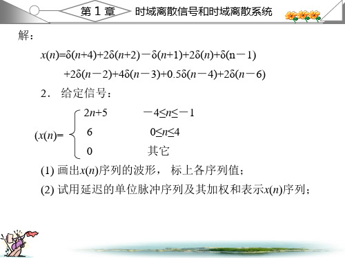
解:
x(n)=δ(n+4)+2δ(n+2)-δ(n+1)+2δ(n)+δ(n-1)
+2δ(n-2)+4δ(n-3)+0.5δ(n-4)+2δ(n-6)
2. 给定信号:
2n+5
-4≤n≤-1
(x(n)= 6 0
0≤n≤4 其它
(1) 画出x(n)序列的波形, 标上各序列值;
(2) y(n)=x(n)+x(n+1)
n n0
(3) y(n)= x(k) k nn0
(4) y(n)=x(n-n0) (5) y(n)=ex(n)
第 1 章 时域离散信号和时域离散系统
解:(1)只要N≥1, 该系统就是因果系统, 因为输出 只与n时刻的和n时刻以前的输入有关。
如果|x(n)|≤M, 则|y(n)|≤M, (2) 该系统是非因果系统, 因为n时间的输出还和n时间以 后((n+1)时间)的输入有关。如果|x(n)|≤M, 则 |y(n)|≤|x(n)|+|x(n+1)|≤2M,
第 1 章 时域离散信号和时域离散系统 题2解图(四)
数字信号处理上机实验答案(全)1

第十章上机实验数字信号处理是一门理论和实际密切结合的课程,为深入掌握课程内容,最好在学习理论的同时,做习题和上机实验。
上机实验不仅可以帮助读者深入的理解和消化基本理论,而且能锻炼初学者的独立解决问题的能力。
本章在第二版的基础上编写了六个实验,前五个实验属基础理论实验,第六个属应用综合实验。
实验一 系统响应及系统稳定性。
实验二 时域采样与频域采样。
实验三 用FFT 对信号作频谱分析。
实验四 IIR 数字滤波器设计及软件实现。
实验五 FIR 数字滤波器设计与软件实现实验六 应用实验——数字信号处理在双音多频拨号系统中的应用任课教师根据教学进度,安排学生上机进行实验。
建议自学的读者在学习完第一章后作实验一;在学习完第三、四章后作实验二和实验三;实验四IIR 数字滤波器设计及软件实现在。
学习完第六章进行;实验五在学习完第七章后进行。
实验六综合实验在学习完第七章或者再后些进行;实验六为综合实验,在学习完本课程后再进行。
10.1 实验一: 系统响应及系统稳定性1.实验目的(1)掌握 求系统响应的方法。
(2)掌握时域离散系统的时域特性。
(3)分析、观察及检验系统的稳定性。
2.实验原理与方法在时域中,描写系统特性的方法是差分方程和单位脉冲响应,在频域可以用系统函数描述系统特性。
已知输入信号可以由差分方程、单位脉冲响应或系统函数求出系统对于该输入信号的响应,本实验仅在时域求解。
在计算机上适合用递推法求差分方程的解,最简单的方法是采用MA TLAB 语言的工具箱函数filter 函数。
也可以用MATLAB 语言的工具箱函数conv 函数计算输入信号和系统的单位脉冲响应的线性卷积,求出系统的响应。
系统的时域特性指的是系统的线性时不变性质、因果性和稳定性。
重点分析实验系统的稳定性,包括观察系统的暂态响应和稳定响应。
系统的稳定性是指对任意有界的输入信号,系统都能得到有界的系统响应。
或者系统的单位脉冲响应满足绝对可和的条件。
数字信号处理实验答案完整版

数字信号处理实验答案 HEN system office room 【HEN16H-HENS2AHENS8Q8-HENH1688】实验一熟悉Matlab环境一、实验目的1.熟悉MATLAB的主要操作命令。
2.学会简单的矩阵输入和数据读写。
3.掌握简单的绘图命令。
4.用MATLAB编程并学会创建函数。
5.观察离散系统的频率响应。
二、实验内容认真阅读本章附录,在MATLAB环境下重新做一遍附录中的例子,体会各条命令的含义。
在熟悉了MATLAB基本命令的基础上,完成以下实验。
上机实验内容:(1)数组的加、减、乘、除和乘方运算。
输入A=[1 2 3 4],B=[3 4 5 6],求C=A+B,D=A-B,E=A.*B,F=A./B,G=A.^B并用stem语句画出A、B、C、D、E、F、G。
clear all;a=[1 2 3 4];b=[3 4 5 6];c=a+b;d=a-b;e=a.*b;f=a./b;g=a.^b;n=1:4;subplot(4,2,1);stem(n,a);xlabel('n');xlim([0 5]);ylabel('A');subplot(4,2,2);stem(n,b);xlabel('n');xlim([0 5]);ylabel('B');subplot(4,2,3);stem(n,c);xlabel('n');xlim([0 5]);ylabel('C');subplot(4,2,4);stem(n,d);xlabel('n');xlim([0 5]);ylabel('D');subplot(4,2,5);stem(n,e);xlabel('n');xlim([0 5]);ylabel('E');subplot(4,2,6);stem(n,f);xlabel('n');xlim([0 5]);ylabel('F');subplot(4,2,7);stem(n,g);xlabel('n');xlim([0 5]);ylabel('G');(2)用MATLAB实现下列序列:a) x(n)= 0≤n≤15b) x(n)=e+3j)n 0≤n≤15c) x(n)=3cosπn+π)+2sinπn+π) 0≤n≤15(n)=x(n+16),绘出四个周期。
程佩青《数字信号处理教程》(第4版)(课后习题详解 无限长单位冲激响应(IIR))
7.2 课后习题详解7-1 用冲激响应不变法将以下Ha (s )变换为H (z ),抽样周期为T 。
(1)H a (s )=(s +a )/[(s +a )2+b 2];(2)H a (s )=A/(s -s 0)n0,n 0为任意正整数。
解:(1)冲激响应不变法满足h (n )=h a (t )|t =nT =h a (nT ),T 为抽样间隔。
这种变换法必须让H a (s )先用部分分式展开。
由推出由冲激响应不变法可得(2)先引用拉氏变换的结论,可得按且可得可以递推求得7-2 设计一个模拟低通滤波器,要求其通带截止频率f p=20Hz,其通带最大衰减为R p=2dB,阻带截止频率为f st=40Hz,阻带最小衰减为A s=20dB,采用巴特沃思滤波器,画出滤波器的幅度响应。
解:巴特沃思模拟低通滤波器设计流程为:①利用教程(7-5-24)式求解滤波器阶次N;②利用教程(7-5-27a)式求解3dB截止频率Ωc;③查教程表7-2或表7-4获得归一化巴特沃思低通滤波器的系统函数H an(s);④将H an(s)根据Ωc的值去归一化求得所需的系统函数H a(s)。
已知Ωp=2π×20rad/s,Ωst=2π×40rad/s,R p=2dB,A s=20dB。
(1)按给定的参数由教程(7-5-24)式可求得取N=4。
(2)按教程(7-5-27a)式可求得巴特沃思滤波器3dB处的通带截止频率Ωc为(3)查教程表7-2可得N=4时归一化巴特沃思低通滤波器H an(s)(4)去归一化,求得所需的H a(s)为滤波器的幅度响应如图7-1所示。
图7-17-3 设计一个模拟高通滤波器,要求其阻带截止频率f st=30Hz,阻带最小衰减为A s=25dB,通带截止频率为f p=50Hz,通带最大衰减为R p=1dB。
(1)采用巴特沃思滤波器;(2)采用切比雪夫滤波器;(3)利用MATLAB工具箱函数设计椭圆函数滤波器。
数字信号处理教程第四版答案

z2 x (n ) [z ]z 0 8 1 (z )z 4
当n 0时,围线内部没有极点 ,故x(n) 0
1 x(n) 7 u(n 1) 8(n) 4
n
z2 部分分式法: X(z) 1 z 4 X(z) z2 A1 A2 故 1 1 z z (z )z z 4 4
数 字 信 号 处 理
第二章 z变换与离散时间傅里叶 变换(DTFT)
2.2 z变换的定义与收敛域
序列x(ห้องสมุดไป่ตู้)的z变换定义为:
n x ( n ) z
X ( z)
n
对任意给定序列x(n),使其z变换收敛的所有z值的集合 称为X(z)的收敛域,上式收敛的充分必要条件是满足绝 对可和
1 z2 A1 [(z ) ] 1 7 1 4 (z )z z 4 4 z2 A 2 [z ] 8 1 z 0 (z )z 4
n
7 1 X( z ) 8,| z | 1 1 4 1 z 4
1 x(n) 7 u(n 1) 8(n) 4
1 | z | 4
n 1
jIm[z]
1/4 o
Re[z]
当n 1时,分母中z的阶次比分子中 z的阶次高两阶 或两阶以上,可用围线 外部极点求解
1 (z 2)z n 1 1 n x (n ) [(z ) ] 1 7( ) z 1 4 4 4 z 4
z2 当n 0时,F(z) ,此时围线内部有一阶 极点z 0 1 (z )z 4
1 n x (n ) ( ) u (n ) 2
部分分式法: Z[a n u (n )]
1 , | z || a | 1 1 az
数字信号处理第四版高西全课后答案
第 1 章 时域离散信号和时域离散系统
(6) y(n)=x(n2)
令输入为
输出为
x(n-n0)
y′(n)=x((n-n0)2) y(n-n0)=x((n-n0)2)=y′(n) 故系统是非时变系统。 由于
T[ax1(n)+bx2(n)]=ax1(n2)+bx2(n2) =aT[x1(n)]+bT[x2(n)]
5. 设系统分别用下面的差分方程描述, x(n)与y(n)分别表示系统输入和输 出, 判断系统是否是线性非时变的。
(1)y(n)=x(n)+2x(n-1)+3x(n-2) (2)y(n)=2x(n)+3 (3)y(n)=x(n-n0) n0 (4)y(n)=x(-n)
第 1 章 时域离散信号和时域离散系统
, 这是2π有理1数4, 因此是周期序
3
(2) 因为ω=
,
所以
1
8
=16π, 这是无理数, 因此是非周期序列。
2π
第 1 章 时域离散信号和时域离散系统
4. 对题1图给出的x(n)要求:
(1) 画出x(-n)的波形;
(2) 计算xe(n)= (3) 计算xo(n)=
1 2 [x(n)+x(-n)], 并画出xe(n)波形; 1 [x(n)-x(-n)], 并画出xo(n)波形; 2
(5) 系统是因果系统, 因为系统的输出不取决于x(n)的未来值。 如果
|x(n)|≤M, 则|y(n)|=|ex(n)|≤e|x(n)|≤eM,
7. 设线性时不变系统的单位脉冲响应h(n)和输入序列x(n)如题7图所示,
要求画出y(n)输出的波形。
解: 解法(一)采用列表法。
数字信号处理米特拉第四版实验一答案
Name : SOLUTION Section :Laboratory Exercise 1DISCRETE-TIME SIGNALS: TIME-DOMAIN REPRESENTATION1.1GENERATION OF SEQUENCESProject 1.1Unit sample and unit step sequencesA copy of Program P1_1 is given below.% Program P1_1% Generation of a Unit Sample Sequence clf;% Generate a vector from -10 to 20 n = -10:20;% Generate the unit sample sequence u = [zeros(1,10) 1 zeros(1,20)]; % Plot the unit sample sequence stem(n,u);xlabel('Time index n');ylabel('Amplitude'); title('Unit Sample Sequence'); axis([-10 20 0 1.2]); Answers : Q1.1The unit sample sequence u[n] generated by running Program P1_1 is shown below:Time index nA m p l i t u d eUnit Sample SequenceQ1.2The purpose of clf command is – clear the current figureThe purpose of axis command is – control axis scaling and appearanceThe purpose of title command is – add a title to a graph or an axis and specify textpropertiesThe purpose of xlabel command is – add a label to the x-axis and specify textpropertiesThe purpose of ylabel command is – add a label to the y-axis and specify the textpropertiesQ1.3The modified Program P1_1 to generate a delayed unit sample sequence ud[n] with a delay of 11 samples is given below along with the sequence generated by running this program .% Program P1_1, MODIFIED for Q1.3% Generation of a DELAYED Unit Sample Sequence clf;% Generate a vector from -10 to 20 n = -10:20;% Generate the DELAYED unit sample sequence u = [zeros(1,21) 1 zeros(1,9)];% Plot the DELAYED unit sample sequence stem(n,u);xlabel('Time index n');ylabel('Amplitude'); title('DELAYED Unit Sample Sequence'); axis([-10 20 0 1.2]);Time index nA m p l i t u d eDELAYED Unit Sample SequenceQ1.4The modified Program P1_1 to generate a unit step sequence s[n] is given below along with the sequence generated by running this program .% Program Q1_4% Generation of a Unit Step Sequence clf;% Generate a vector from -10 to 20 n = -10:20;% Generate the unit step sequence s = [zeros(1,10) ones(1,21)]; % Plot the unit step sequence stem(n,s);xlabel('Time index n');ylabel('Amplitude'); title('Unit Step Sequence'); axis([-10 20 0 1.2]);Time index nA m p l i t u d eUnit Step SequenceQ1.5The modified Program P1_1 to generate a unit step sequence sd[n] with an advance of 7 samples is given below along with the sequence generated by running this program .% Program Q1_5% Generation of an ADVANCED Unit Step Sequence clf;% Generate a vector from -10 to 20 n = -10:20;% Generate the ADVANCED unit step sequence sd = [zeros(1,3) ones(1,28)];% Plot the ADVANCED unit step sequence stem(n,sd);xlabel('Time index n');ylabel('Amplitude'); title('ADVANCED Unit Step Sequence'); axis([-10 20 0 1.2]);Time index nA m p l i t u d eADVANCED Unit Step SequenceProject 1.2 Exponential signalsA copy of Programs P1_2 and P1_3 are given below .% Program P1_2% Generation of a complex exponential sequence clf;c = -(1/12)+(pi/6)*i; K = 2; n = 0:40;x = K*exp(c*n); subplot(2,1,1); stem(n,real(x));xlabel('Time index n');ylabel('Amplitude'); title('Real part'); subplot(2,1,2); stem(n,imag(x));xlabel('Time index n');ylabel('Amplitude'); title('Imaginary part');% Program P1_3% Generation of a real exponential sequence clf;n = 0:35; a = 1.2; K = 0.2; x = K*a.^n; stem(n,x);xlabel('Time index n');ylabel('Amplitude');Answers: Q1.6The complex-valued exponential sequence generated by running Program P1_2 is shown below :510152025303540Time index n A m p l i t u d eReal partTime index nA m p l i t u d eImaginary partQ1.7The parameter controlling the rate of growth or decay of this sequence is – the real part of c .The parameter controlling the amplitude of this sequence is - KQ1.8The result of changing the parameter c to (1/12)+(pi/6)*i is – since exp(-1/12) isless than one and exp(1/12) is greater than one, this change means that the envelope of the signal will grow with n instead of decay with n.Q1.9The purpose of the operator real is – to extract the real part of a Matlab vector.The purpose of the operator imag is – to extract the imaginary part of a Matlab vector. Q1.10The purpose of the command subplot is – to plot more than one graph in the sameMatlab figure.Q1.11The real-valued exponential sequence generated by running Program P1_3 is shown below :Time index nA m p l i t u d eQ1.12The parameter controlling the rate of growth or decay of this sequence is - aThe parameter controlling the amplitude of this sequence is - KQ1.13The difference between the arithmetic operators ^ and .^ is – “^” raises a square matrix toa power using matrix multiplication. “.^” raises the elements of a matrix or vector to a power; this is a “pointwise” operation.Q1.14The sequence generated by running Program P1_3 with the parameter a changed to 0.9 and the parameter K changed to 20 is shown below :5101520253035Time index nA m p l i t u d eQ1.15The length of this sequence is - 36It is controlled by the following MATLAB command line : n = 0:35;It can be changed to generate sequences with different lengths as follows (give an example command line and the corresponding length): n = 0:99; makes the length 100. Q1.16The energies of the real-valued exponential sequences x [n]generated in Q1.11 and Q1.14 and computed using the command sum are - 4.5673e+004 and 2.1042e+003.Project 1.3 Sinusoidal sequencesA copy of Program P1_4 is given below .% Program P1_4% Generation of a sinusoidal sequence n = 0:40;f = 0.1; phase = 0; A = 1.5; arg = 2*pi*f*n - phase; x = A*cos(arg);clf; % Clear old graphstem(n,x); % Plot the generated sequence axis([0 40 -2 2]); grid;title('Sinusoidal Sequence'); xlabel('Time index n'); ylabel('Amplitude'); axis; Answers:Q1.17 The sinusoidal sequence generated by running Program P1_4 is displayed below .0510152025303540Sinusoidal SequenceTime index nA m p l i t u d eQ1.18The frequency of this sequence is- f = 0.1 cycles/sample.It is controlled by the following MATLAB command line: f = 0.1;A sequence with new frequency 0.2 can be generated by the following command line:f = 0.2;The parameter controlling the phase of this sequence is- phaseThe parameter controlling the amplitude of this sequence is- AThe period of this sequence is - 2π/ω = 1/f = 10Q1.19 The length of this sequence is - 41It is controlled by the following MATLAB command line: n = 0:40;A sequence with new length __81_ can be generated by the following command line:n = 0:80;Q1.20 The average power of the generated sinusoidal sequence is–sum(x(1:10).*x(1:10))/10 = 1.1250Q1.21 The purpose of axis command is – to set the range of the x-axis to [0,40] and the range of the y-axis to [-2,2].The purpose of grid command is – to turn on the drawing of grid lines on the graph.Q1.22 The modified Program P1_4 to generate a sinusoidal sequence of frequency 0.9 is given below along with the sequence generated by running it.% Program Q1_22A% Generation of a sinusoidal sequencen = 0:40;f = 0.9;phase = 0;A = 1.5;arg = 2*pi*f*n - phase;x = A*cos(arg);clf; % Clear old graphstem(n,x); % Plot the generated sequenceaxis([0 40 -2 2]);grid;title('Sinusoidal Sequence');xlabel('Time index n');ylabel('Amplitude');axis;Sinusoidal SequenceTime index nA m p l i t u d eA comparison of this new sequence with the one generated in Question Q1.17 shows - thetwo graphs are identical. This is because, in the modified program, we have ω = 0.9*2π. This generates the same graph as a cosine with angular frequency ω - 2π = −0.1*2π. Because cosine is an even function, this is the same as a cosine with angular frequency +0.1*2π, which was the value used in P1_4.m in Q1.17.In terms of Hertzian frequency, we have for P1_4.m in Q1.17 that f = 0.1 Hz/sample. For the modified program in Q1.22, we have f = 0.9 Hz/sample, which generates the same graph as f = 0.9 – 1 = −0.1. Again because cosine is even, this makes a graph that is identical to the one we got in Q1.17 with f = +0.1 Hz/sample.A sinusoidal sequence of frequency 1.1 generated by modifying Program P1_4 is shown below.0510152025303540Sinusoidal SequenceTime index nA m p l i t u d eA comparison of this new sequence with the one generated in Question Q1.17 shows - thegraph here is again identical to the one in Q1.17. This is because a cosine of frequency f = 1.1 Hz/sample is identical to one with frequency f = 1.1 – 1 = 0.1 Hz/sample, which was the frequency used in Q1.17.Q1.23The sinusoidal sequence of length 50, frequency 0.08, amplitude 2.5, and phase shift of 90 degrees generated by modifying Program P1_4 is displayed below .NOTE: for this program, it is necessary to convert the phase of 90 deg to radians and account for the minus sign that appears in the statement “arg = 2*pi*f*n - phase;” as opposed to the plus sign shown in eq. (1.12) of the lab manual. The correct statement to generate the phase is “phase = -90/(2*pi);”. It is also necessary to modify the axis command to account for the new length and amplitude of the signal. The correct axis statement is “axis([0 50 -3 3]);”.05101520253035404550Sinusoidal SequenceTime index nA m p l i t u d eThe period of this sequence is - 2π/ω = 1/f = 1/0.08 = 1/(8/100) = 100/8 = 25/2.Therefore, the fundamental period is 25 and the graph has the “appearance” of going through 2 cycles of a cosine waveform during each period.Q1.24By replacing the stem command in Program P1_4 with the plot command, the plot obtained is as shown below :Sinusoidal SequenceTime index nA m p l i t u d eThe difference between the new plot and the one generated in Question Q1.17 is – instead ofdrawing stems from the x-axis to the points on the curve, the “plot ” command connects the points with straight line segments, which approximates the graph of a continuous-time cosine signal.Q1.25By replacing the stem command in Program P1_4 with the stairs command the plot obtained is as shown below :Sinusoidal SequenceTime index nA m p l i t u d eThe difference between the new plot and those generated in Questions Q1.17 and Q1.24 is– the “stairs” command produces a stairstep plot as opposed to the stem graph that was generated in Q1.17 and the straight-line interpolation plot that was generated in Q1.24.Project 1.4 Random signalsAnswers:Q1.26 The MATLAB program to generate and display a random signal of length 100 with elements uniformly distributed in the interval [–2, 2] is given below along with the plot of the random sequence generated by running the program:% Program Q1_26% Generation of a uniform random sequencen = 0:99;A = 2;rand('state',sum(100*clock)); % "seed" the generator% rand(1,100) is uniform in [0,1]% rand(1,100)-0.5 is uniform in [-0.5,0.5]% 4*(rand(1,100)-0.5) is uniform in [-2,2]x = 2*A*(rand(1,length(n))-0.5);clf; % Clear old graphstem(n,x); % Plot the generated sequenceaxis([0 length(n) -round(2*(A+0.5))/2 round(2*(A+0.5))/2]);grid;title('Uniform Random Sequence');xlabel('Time index n');ylabel('Amplitude');axis;102030405060708090100Uniform Random SequenceTime index nA m p l i t u d eQ1.27 The MATLAB program to generate and display a Gaussian random signal of length 75 withelements normally distributed with zero mean and a variance of 3 is given below along with the plot of the random sequence generated by running the program :% Program Q1_27% Generation of a Gaussian random sequence% NOTE: if X is a random variable with zero mean and % unity variance, then (aX + b) is a random variable % with mean b and variance a^2. This follows from % basic probability theory. n = 0:74;xmean = 0; % mean of xxstd = sqrt(3); % standard deviation of xrandn('state',sum(100*clock)); % "seed" the generator % generate the sequencex = xstd*randn(1,length(n)) + xmean; % setup the graph and plotclf; % Clear old graphstem(n,x); % Plot the generated sequence xmax = max(abs(x));Ylim = round(2*(xmax+0.5))/2; axis([0 length(n) -Ylim Ylim]); grid;title('Gaussian Random Sequence'); xlabel('Time index n'); ylabel('Amplitude'); axis;10203040506070Gaussian Random SequenceTime index nA m p l i t u d eQ1.28The MATLAB program to generate and display five sample sequences of a random sinusoidal signal of length 31{X[n]} = {A·cos(ωo n + φ)}where the amplitude A and the phase φ are statistically independent random variables with uniform probability distribution in the range 0≤A ≤4 for the amplitude and in the range 0 ≤ φ ≤ 2π for the phase is given below. Also shown are five sample sequences generated by running this program five different times .% Generates the "deterministic stochastic process" % called for in Q1.28. n = 0:30; f = 0.1; Amax = 4;phimax = 2*pi;rand('state',sum(100*clock)); % "seed" the generator A = Amax*rand;% NOTE: successive calls to rand without arguments % return a random sequence of scalars. Since this % random sequence is "white" (uncorrelated), it is % not necessary to re-seed the generator for phi. phi = phimax*rand;% generate the sequence arg = 2*pi*f*n + phi; x = A*cos(arg); % plotclf; % Clear old graphstem(n,x); % Plot the generated sequence Ylim = round(2*(Amax+0.5))/2; axis([0 length(n) -Ylim Ylim]); grid;title('Sinusoidal Sequence with Random Amplitude and Phase'); xlabel('Time index n'); ylabel('Amplitude'); axis;Sinusoidal Sequence with Random Amplitude and PhaseTime index nA m p l i t u d eSinusoidal Sequence with Random Amplitude and PhaseTime index nA m p l i t u d eTime index nA m p l i t u d eSinusoidal Sequence with Random Amplitude and PhaseTime index nA m p l i t u d eTime index nA m p l i t u d e1.2 SIMPLE OPERATIONS ON SEQUENCESProject 1.5Signal SmoothingA copy of Program P1_5 is given below .% Program P1_5% Signal Smoothing by Averaging clf; R = 51;d = 0.8*(rand(R,1) - 0.5); % Generate random noise m = 0:R-1;s = 2*m.*(0.9.^m); % Generate uncorrupted signal x = s + d'; % Generate noise corrupted signal subplot(2,1,1);plot(m,d','r-',m,s,'g--',m,x,'b-.');xlabel('Time index n');ylabel('Amplitude'); legend('d[n] ','s[n] ','x[n] ');x1 = [0 0 x];x2 = [0 x 0];x3 = [x 0 0]; y = (x1 + x2 + x3)/3; subplot(2,1,2);plot(m,y(2:R+1),'r-',m,s,'g--'); legend( 'y[n] ','s[n] ');xlabel('Time index n');ylabel('Amplitude'); Answers: Q1.29The signals generated by running Program P1_5 are displayed below :05101520253035404550-5510Time index nA m p l i t u d e2468Time index nA m p l i t u d eQ1.30The uncorrupted signal s[n]is - the product of a linear growth with a slowly decayingreal exponential.The additive noise d[n]is – a random sequence uniformly distributed between -0.4 and+0.4.Q1.31 The statement x = s + d CANNOT be used to generate the noise corrupted signalbecause – d is a column vector, whereas s is a row vector; it is necessary to transposeone of these vectors before adding them.Q1.32The relations between the signals x1, x2, and x3, and the signal x are – all three signalsx1, x2, and x3 are extended versions of x , with one additional sample appended at the left and one additional sample appended to the right. The signal x1 is a delayedversion of x , shifted one sample to the right with zero padding on the left. The signal x2 is equal to x , with equal zero padding on both the left and right to account for the extended length. Finally, x3 is a time advanced version of x , shifted one sample to the left with zero padding on the right.Q1.33The purpose of the legend command is – to create a legend for the graphs. In P1_5, the signals are plotted using different colors and line types; the legend providesinformation about which color and line type is associated with each signal.Project 1.6Generation of Complex SignalsA copy of Program P1_6 is given below.% Program P1_6% Generation of amplitude modulated sequenceclf;n = 0:100;m = 0.4;fH = 0.1; fL = 0.01;xH = sin(2*pi*fH*n);xL = sin(2*pi*fL*n);y = (1+m*xL).*xH;stem(n,y);grid;xlabel('Time index n');ylabel('Amplitude');Answers:Q1.34 The amplitude modulated signals y[n]generated by running Program P1_6 for various values of the frequencies of the carrier signal xH[n]and the modulating signal xL[n], andvarious values of the modulation index m are shown below:m=0.4; fH=0.1; fL=0.01:Time index nA m p l i t u d em=0.9; fH=0.1; fL=0.1:Time index nA m p l i t u d em=0.4; fH=0.1; fL=0.005:Time index nA m p l i t u d em=0.4; fH=0.25; fL=0.01:Time index nA m p l i t u d eQ1.35 The difference between the arithmetic operators * and .* is – “*” multiplies twoconformable matrices or vectors using matrix multiplication. “.*” takes the pointwise products of the elements of two matrices or vectors that have the same dimensions.A copy of Program P1_7 is given below .% Program P1_7% Generation of a swept frequency sinusoidal sequence n = 0:100; a = pi/2/100; b = 0;arg = a*n.*n + b*n; x = cos(arg);clf; stem(n, x);axis([0,100,-1.5,1.5]);title('Swept-Frequency Sinusoidal Signal'); xlabel('Time index n'); ylabel('Amplitude'); grid; axis; Answers:Q1.36 The swept-frequency sinusoidal sequence x[n] generated by running Program P1_7 isdisplayed below .Swept-Frequency Sinusoidal SignalTime index nA m p l i t u d eQ1.37The minimum and maximum frequencies of this signal are - The minimum occurs at n=0, where we have 2an+b = 0 rad/sample = 0 Hz/sample. The maximum occurs at n=100, where we have 2an+b = 200a = 200π(0.5)(0.01) = π rad/sample= 0.5 Hz/sample.Q1.38The Program 1_7 modified to generate a swept sinusoidal signal with a minimum frequency of0.1 and a maximum frequency of 0.3 is given below:Note: for a minimum frequency of 0.1 Hz/sample = π/5 rad/sample at n=0, we must have 2a(0) + b =π/5, which implies b=π/5. For a maximum frequency of 0.3 Hz/sample = 3π/5 rad/sample at n=100, we must have 2a(100) + π/5 = 3π/5, which implies a=π/500.% Program Q1_38% Generation of a swept frequency sinusoidal sequencen = 0:100;a = pi/500;b = pi/5;arg = a*n.*n + b*n;x = cos(arg);clf;stem(n, x);axis([0,100,-1.5,1.5]);title('Swept-Frequency Sinusoidal Signal');xlabel('Time index n');ylabel('Amplitude');grid; axis;INFORMATION1.3 WORKSPACEQ1.39The information displayed in the command window as a result of the who command is – a listing of the names of the variables defined in the current workspace.Q1.40The information displayed in the command window as a result of the whos command is – a long form listing of the variables defined in the current workspace, including the variable names, their dimensions (size), the number of bytes of storage required for each variable, and the datatype of each variable. The total number of bytes of storagefor the entire workspace is also displayed.1.4 OTHER TYPES OF SIGNALS (Optional)Project 1.8 Squarewave and Sawtooth SignalsAnswer:Q1.41MATLAB programs to generate the square-wave and the sawtooth wave sequences of the type shown in Figures 1.1 and 1.2 are given below along with the sequences generated by running these programs:% Program Q1_41A% Generation of the square wave in Fig. 1.1(a)n = 0:30;f = 0.1;phase = 0;duty=60;A = 2.5;arg = 2*pi*f*n + phase;x = A*square(arg,duty);clf; % Clear old graphstem(n,x); % Plot the generated sequenceaxis([0 30 -3 3]);grid;title('Square Wave Sequence of Fig. 1.1(a)');xlabel('Time index n');ylabel('Amplitude');axis;% Program Q1_41B% Generation of the square wave in Fig. 1.1(b)n = 0:30;f = 0.1;phase = 0;duty=30;A = 2.5;arg = 2*pi*f*n + phase;x = A*square(arg,duty);clf; % Clear old graphstem(n,x); % Plot the generated sequenceaxis([0 30 -3 3]);grid;title('Square Wave Sequence of Fig. 1.1(b)');xlabel('Time index n');ylabel('Amplitude');axis;% Program Q1_41C% Generation of the square wave in Fig. 1.2(a) n = 0:50;f = 0.05;phase = 0;peak = 1;A = 2.0;arg = 2*pi*f*n + phase;x = A*sawtooth(arg,peak);clf; % Clear old graphstem(n,x); % Plot the generated sequence axis([0 50 -2 2]);grid;title('Sawtooth Wave Sequence of Fig. 1.2(a)'); xlabel('Time index n');ylabel('Amplitude');axis;% Program Q1_41D% Generation of the square wave in Fig. 1.2(b) n = 0:50;f = 0.05;phase = 0;peak = 0.5;A = 2.0;arg = 2*pi*f*n + phase;x = A*sawtooth(arg,peak);clf; % Clear old graphstem(n,x); % Plot the generated sequence axis([0 50 -2 2]);grid;title('Sawtooth Wave Sequence of Fig. 1.2(b)'); xlabel('Time index n');ylabel('Amplitude');axis;051015202530Time index nA m p l i t u d eSquare Wave Sequence of Fig. 1.1(b)Time index nA m p l i t u d eTime index nA m p l i t u d eSawtooth Wave Sequence of Fig. 1.2(b)Time index nA m p l i t u d eDate: 14 September, 2006 Signature: HAVLICEK。
数字信号处理习题答案及matlab实验详解.pdf
Z = 0,0.8361,0.4306 P =1.0000, 0.6000,0.3000
(2)
由于 H (z)
Y (z) X (z)
1
3 1.9
3.8z1 1.08 z1 1.08z2
z 2 0.18z
3
所以系统的差分方程:
y(n) 1.9 y(n 1) 1.08 y(n 2) 0.18 y(n 3) 3x(n) 3.8x(n 1) 1.08x(n 2)
1 2
n
u(n),
x
2
(n)
1 3
n
u
(n)
利用 Z 变换性质求 y(n)的 Z 变换 Y(Z)。
实验 2-1 离散系统的分析的基本理论 实验目的:加深对离散系统基本理论和方法的理解
1 一线性移不变离散时间系统的单位抽样响应为 h(n) (1 0.3n 0.6n )u(n)
(1) 求该系统的转移函数 H (z) ,并画出其零-极点图; (2) 写出该系统的差分方程。
阶跃响应为: y[n] x[n] h[n] x[m]h[n m] h(n m), n m, m 0
m
m0
即 y(0) 0, y(1) 0.25, y(2) 0.5, y(3) 0.75,其余y(n) 1, (n 3)
利用函数 h=impz(b,a,N)和 y=filter(b,a,x)分别绘出冲激和阶跃响应 b=[0,0.25,0.25,0.25,0.25]; a=1; x=ones(1,100); h=impz(b,a,100);y=filter(b,a,x) figure(1) subplot(2,1,1); stem(h,’.’); subplot(2,1,2); plot(y,’.’);
数字信号处理参考答案
数字信号处理参考答案《解答题及分析题》一、解释下列名词:(1)DSP: 数字信号处理或者数字信号处理芯片;(2)MIPS: 每秒执行百万条指令 ;(3)MOPS: 每秒执行百万条操作 ;(4)FFT: 快速傅里叶变换 ;(5)MAC 时间: 完成一次乘法和一次加法的时间 ;(6)指令周期:执行一条指令所需要的时间,单位通常为(ns );(7)BOPS:每秒执行十亿次操作;(8)MFLOPS :每秒执行百万次浮点操作;(9)TMS320C54X :TI 公司的54系列定点DSP 芯片;(10)ADSP21XX:AD :公司的21系列定点DSP 芯片;二、已知)()()]([n x n g n x T =判断系统是否为:① 因果系统;② 稳定系统;③ 线性系统;④ 移不变系统解:(1)求解系统的单位取样响应)(n h令)()(n n x δ=,则系统的单位取样响应)()()(n n g n h δ=① 当0<n 时,0)(=n h ,系统为因果系统;②0)(=∑+∞-∞=n n h ,是稳定系统; ③ 设)()()(),()()(2211n g n x n y n g n x n y ==由于)()()()([)(2121n by n ay n bx n ax T n y +=+=,④ 由于)()]([),()()(k n y k n X T k n g k n x k n y -≠---=-而, 因此,系统为移变系统。
其余几个题的判断方法与这个相同,略。
三、画方框图说明DSP 系统的设计步骤。
设计步骤:(1)根据实际问题的要求写出任务书确定设计目标;(2)算法研究并确定系统的性能指标;(3)选择DSP 芯片和外围芯片;(4)完成系统的硬件设计和软件设计;(5)完成系统的硬件仿真和软件调试;(6)系统集成和测试。
四、以TMS320C5402为例,说明一个典型的DSP 实时数字信号处理系统通常有哪些部分组成?画出系统组成的方框图。
- 1、下载文档前请自行甄别文档内容的完整性,平台不提供额外的编辑、内容补充、找答案等附加服务。
- 2、"仅部分预览"的文档,不可在线预览部分如存在完整性等问题,可反馈申请退款(可完整预览的文档不适用该条件!)。
- 3、如文档侵犯您的权益,请联系客服反馈,我们会尽快为您处理(人工客服工作时间:9:00-18:30)。
Section:
Laboratory Exercise 1
DISCRETE-TIME SIGNALS: TIME-DOMAIN REPRESENTATION
1.1 GENERATION OF SEQUENCES
Project 1.1 Unit sample and unit step sequences
Imaginary part 2
Amplitude
1
0
-1
0
5
10
15
20
25
30
35
40
Time index n
Q1.7 The parameter controlling the rate of growth or decay of this sequence is – the real part of c.
4
Answers:
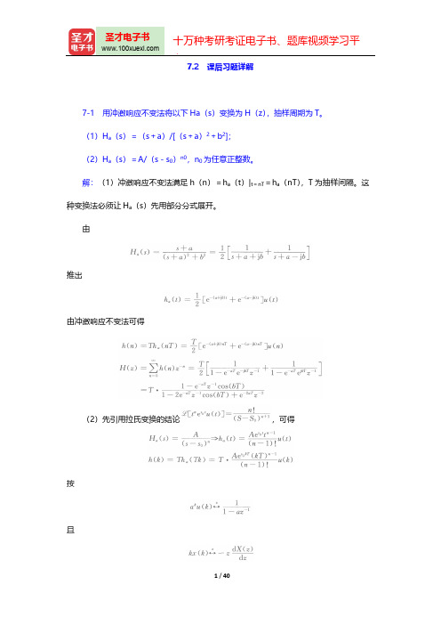
Q1.6
The complex-valued exponential sequence generated by running Program P1_2 is shown
below:
Amplitude
Real part 2
1
0
-1
-2
0
51015ຫໍສະໝຸດ 202530
35
40
Time index n
% Program Q1_4 % Generation of a Unit Step Sequence clf; % Generate a vector from -10 to 20 n = -10:20; % Generate the unit step sequence s = [zeros(1,10) ones(1,21)]; % Plot the unit step sequence stem(n,s); xlabel('Time index n');ylabel('Amplitude'); title('Unit Step Sequence'); axis([-10 20 0 1.2]);
% Program P1_1, MODIFIED for Q1.3 % Generation of a DELAYED Unit Sample Sequence clf; % Generate a vector from -10 to 20 n = -10:20; % Generate the DELAYED unit sample sequence u = [zeros(1,21) 1 zeros(1,9)]; % Plot the DELAYED unit sample sequence stem(n,u); xlabel('Time index n');ylabel('Amplitude'); title('DELAYED Unit Sample Sequence'); axis([-10 20 0 1.2]);
properties
Q1.3
The modified Program P1_1 to generate a delayed unit sample sequence ud[n] with a delay of 11 samples is given below along with the sequence generated by running this program.
Q1.9 The purpose of the operator real is – to extract the real part of a Matlab vector.
Q1.10
The purpose of the operator imag is – to extract the imaginary part of a Matlab vector.
% Program Q1_5 % Generation of an ADVANCED Unit Step Sequence clf; % Generate a vector from -10 to 20 n = -10:20; % Generate the ADVANCED unit step sequence sd = [zeros(1,3) ones(1,28)]; % Plot the ADVANCED unit step sequence stem(n,sd); xlabel('Time index n');ylabel('Amplitude'); title('ADVANCED Unit Step Sequence'); axis([-10 20 0 1.2]);
18
16
14
12
10
8
6
4
2
0
0
5
10
15
20
25
30
35
Time index n
Q1.15 The length of this sequence is - 36 It is controlled by the following MATLAB command line: n = 0:35;
3
ADVANCED Unit Step Sequence
Amplitude
1
0.8
0.6
0.4
0.2
0
-10
-5
0
5
10
15
20
Time index n
Project 1.2 Exponential signals
A copy of Programs P1_2 and P1_3 are given below.
% Program P1_3 % Generation of a real exponential sequence clf; n = 0:35; a = 1.2; K = 0.2; x = K*a.^n; stem(n,x); xlabel('Time index n');ylabel('Amplitude');
% Program P1_2 % Generation of a complex exponential sequence clf; c = -(1/12)+(pi/6)*i; K = 2; n = 0:40; x = K*exp(c*n); subplot(2,1,1); stem(n,real(x)); xlabel('Time index n');ylabel('Amplitude'); title('Real part'); subplot(2,1,2); stem(n,imag(x)); xlabel('Time index n');ylabel('Amplitude'); title('Imaginary part');
6
Q1.14 The sequence generated by running Program P1_3 with the parameter a changed to 0.9 and the parameter K changed to 20 is shown below:
Amplitude
20
The parameter controlling the amplitude of this sequence is - K
Q1.8 The result of changing the parameter c to (1/12)+(pi/6)*i is – since exp(-1/12) is less than one and exp(1/12) is greater than one, this change means that the envelope of the signal will grow with n instead of decay with n.
The purpose of the command subplot is – to plot more than one graph in the same Matlab figure.
5
Q1.11 The real-valued exponential sequence generated by running Program P1_3 is shown below:
Q1.13 The difference between the arithmetic operators ^ and .^ is – “^” raises a square matrix to a power using matrix multiplication. “.^” raises the elements of a matrix or vector to a power; this is a “pointwise” operation.
120
100
80
Amplitude
60
40
20
0
0
5
10
15
20
25
30
35
Time index n
Q1.12 The parameter controlling the rate of growth or decay of this sequence is - a The parameter controlling the amplitude of this sequence is - K
A copy of Program P1_1 is given below.
% Program P1_1 % Generation of a Unit Sample Sequence clf; % Generate a vector from -10 to 20 n = -10:20; % Generate the unit sample sequence u = [zeros(1,10) 1 zeros(1,20)]; % Plot the unit sample sequence stem(n,u); xlabel('Time index n');ylabel('Amplitude'); title('Unit Sample Sequence'); axis([-10 20 0 1.2]);