The intermediate shaft component -design of shaft bearings keys,etc
黏性连接器用作前轮驱动限制滑移差速器对汽车牵引和操纵的影响中英文翻译

外文资料与中文翻译外文资料:The Effect of a Viscous Coupling Used as a Front-Wheel Drive Limited-Slip Differential on Vehicle Traction and Handling1 ABCTRACTThe viscous coupling is known mainly as a driveline component in four wheel drive vehicles. Developments in recent years, however, point toward the probability that this device will become a major player in mainstream front-wheel drive application. Production application in European and Japanese front-wheel drive cars have demonstrated that viscous couplings provide substantial improvements not only in traction on slippery surfaces but also in handing and stability even under normal driving conditions.This paper presents a serious of proving ground tests which investigate the effects of a viscous coupling in a front-wheel drive vehicle on traction and handing. Testing demonstrates substantial traction improvements while only slightly influencing steering torque. Factors affecting this steering torque in front-wheel drive vehicles during straight line driving are described. Key vehicle design parameters are identified which greatly influence the compatibility of limited-slip differentials in front-wheel drive vehicles.Cornering tests show the influence of the viscous coupling on the self steering behavior of a front-wheel drive vehicle. Further testing demonstrates that a vehicle with a viscous limited-slip differential exhibits an improved stability under acceleration and throttle-off maneuvers during cornering.2 THE VISCOUS COUPLINGThe viscous coupling is a well known component in drivetrains. In this paper only a short summary of its basic function and principle shall be given.The viscous coupling operates according to the principle of fluid friction, and is thus dependent on speed difference. As shown in Figure 1 the viscous coupling has slip controlling properties in contrast to torque sensing systems.This means that the drive torque which is transmitted to the front wheels isautomatically controlled in the sense of an optimized torque distribution.In a front-wheel drive vehicle the viscous coupling can be installed inside the differential or externally on an intermediate shaft. The external solution is shown in Figure 2.This layout has some significant advantages over the internal solution. First, there is usually enough space available in the area of the intermediate shaft to provide the required viscous characteristic. This is in contrast to the limited space left in today’s front-axle differentials. Further, only minimal modification to the differential carrier and transmission case is required. In-house production of differentials is thus only slightly affected. Introduction as an option can be made easily especially when the shaft and the viscous unit is supplied as a complete unit. Finally, the intermediate shaft makes it possible to provide for sideshafts of equal length with transversely installed engines which is important to reduce torque steer (shown later in section 4).This special design also gives a good possibility for significant weight and cost reductions of the viscous unit. GKN Viscodrive is developing a low weight and cost viscous coupling. By using only two standardized outer diameters, standardized plates, plastic hubs and extruded material for the housing which can easily be cut to different lengths, it is possible to utilize a wide range of viscous characteristics. An example of this development is shown in Figure 3.3 TRACTION EFFECTSAs a torque balancing device, an open differential provides equal tractive effort to both driving wheels. It allows each wheel to rotate at different speeds during cornering without torsional wind-up. These characteristics, however, can be disadvantageous when adhesion variations between the left and right sides of the road surface (split-μ) limits the t orque transmitted for both wheels to that which can be supported by the low-μ wheel.With a viscous limited-slip differential, it is possible to utilize the higher adhesion potential of the wheel on the high-μsurface. This is schematically shown in Figure 4.When for example, the maximum transmittable torque for one wheel is exceeded on a split-μsurface or during cornering with high lateral acceleration, a speed difference between the two driving wheels occurs. The resulting self-locking torque in the viscous coupling resists any further increase in speed difference and transmits theappropriate torque to the wheel with the better traction potential.It can be seen in Figure 4 that the difference in the tractive forces results in a yawing moment which tries to turn the vehicle in to the low-μside, To keep the vehicle in a straight line the driver has to compensate this with opposite steering input. Though the fluid-friction principle of the viscous coupling and the resulting soft transition from open to locking action, this is easily possible, The appropriate results obtained from vehicle tests are shown in Figure 5.Reported are the average steering-wheel torque Ts and the average corrective opposite steering input required to maintain a straight course during acceleration on a split-μtrack with an open and a viscous differential. The differences between the values with the open differential and those with the viscous coupling are relatively large in comparison to each other. However, they are small in absolute terms. Subjectively, the steering influence is nearly unnoticeable. The torque steer is also influenced by several kinematic parameters which will be explained in the next section of this paper.4 FACTORS AFFECTING STEERING TORQUEAs shown in Figure 6 the tractive forces lead to an increase in the toe-in response per wheel. For differing tractive forces, Which appear when accelerating on split-μwith limited -slip differentials, the toe-in response changes per wheel are also different.Unfortunately, this effect leads to an undesirable turn-in response to the low-μside, i.e. the same yaw direction as caused by the difference in the tractive forces.Reduced toe-in elasticity is thus an essential requirement for the successful front-axle application of a viscous limited-slip differential as well as any other type of limited-slip differential.Generally the following equations apply to the driving forces on a wheelμV T F F =With =T F Tractive Force=V F Vertical Wheel Load=μUtilized Adhesion CoefficientThese driving forces result in steering torque at each wheel via the wheel disturbance level arm “e” and a steering torque difference between the wheels givenby the equation:△e T =()lo H hi H F F e ---••δcosWhere △=e T Steering Torque Differencee=Wheel Disturbance Level Arm=δKing Pin Anglehi=high-μside subscriptlo=low-μside subscriptIn the case of front-wheel drive vehicles with open differentials, △Ts is almost unnoticeable, since the torque bias (lo H hi T F F --/) is no more than 1.35.For applications with limited-slip differentials, however, the influence is significant. Thus the wheel disturbance lever arm e should be as small as possible. Differing wheel loads also lead to an increase in △Te so the difference should also be as small as possible.When torque is transmitted by an articulated CV-Joint, on the drive side (subscript 1) and the driven side (subscript 2),differing secondary moments are produced that must have a reaction in a vertical plane relative to the plane of articulation. The magnitude and direction of the secondary moments (M) are calculated as follows (see Figure 8):Drive side M1 =v v T T ββηtan /)2/tan(2-•Driven side M2 =v v T T ββηtan /)2/tan(2+•With T2 =dyn T r F •ηT =()system Jo T f int ,,2βWhere v β∧=Vertical Articulation Angleβ∧=Resulting Articulation Angledyn r ∧=Dynamic Wheel RadiusηT ∧=Average Torque LossThe component δcos 2•M acts around the king-pin axis (see figure 7) as a steering torque per wheel and as a steering torque difference between the wheels as follows:])tan /2/tan ()sin /2/tan [(cos 22li w hi w T T T T T ----+±=∆νηννηνβββββδwhere ∧=∆βT Steering Torque DifferenceW ∧=Wheel side subscriptIt is therefore apparent that not only differing driving torque but also differing articulations caused by various driveshaft lengths are also a factor. Referring to the moment-polygon in Figure 7, the rotational direction of M2 or βT respectively change, depending on the position of the wheel-center to the gearbox output.For the normal position of the halfshaft shown in Figure 7(wheel-center below the gearbox output joint) the secondary moments work in the same rotational direction as the driving forces. For a modified suspension layout (wheel-center above gearbox output joint, i.e. v βnegative) the secondary moments counteract the moments caused by the driving forces. Thus for good compatibility of the front axle with a limited-slip differential, the design requires: 1) vertical bending angles which are centered around 0=v βor negative (0<v β) with same values of v βon both left and right sides; and 2) sideshafts of equal length.The influence of the secondary moments on the steering is not only limited to the direct reactions described above. Indirect reactions from the connection shaft between the wheel-side and the gearbox-side joint can also arise, as shown below:Figure 9: Indirect Reactions Generated by Halfshaft Articulation in the Vertical PlaneFor transmission of torque without loss and vd vw ββ= both of the secondary moments acting on the connection shaft compensate each other. In reality (with torque loss), however, a secondary moment difference appears:△W D DW M M M 12-=With -+=ηT T T W D 22The secondary moment difference is:=DW M ()VW W VW W VD VD W T T D T w T T ββββηηηtan /2/tan sin /tan 22/2+-++ For reasons of simplification it apply that V VW VD βββ==and ηηηT T T W D == to give △()V V V DW T M βββηtan /1sin /12/tan ++•=△DW M requires opposing reaction forces on both joints where L M F DW DW /∆=. Due to the joint disturbance lever arm f, a further steering torque also acts around the king-pin axis:L f M T DW f /cos δ••∆=()lo lo DW hi hi DW f L M L M f T //cos ---••=∆Where ∧=f T Steering Torque per Wheel∧=∆f T Steering Torque Difference∧=f Joint Disturbance Lever∧=L Connection shaft (halfshaft) LengthFor small values of f, which should be ideally zero, f T ∆ is of minor influence.5.EFFECT ON CORNERINGViscous couplings also provide a self-locking torque when cornering, due to speed differences between the driving wheels. During steady state cornering, as shown in figure 10, the slower inside wheel tends to be additionally driven through the viscous coupling by the outside wheel.Figure 10: Tractive forces for a front-wheel drive vehicle during steady state corneringThe difference between the Tractive forces Dfr and Dfl results in a yaw moment MCOG , which has to be compensated by a higher lateral force, and hence a larger slip angle af at the front axle. Thus the influence of a viscous coupling in a front-wheel drive vehicle on self-steering tends towards an understeering characteristic. This behavior is totally consistent with the handling bias of modern vehicles which all under steer during steady state cornering maneuvers. Appropriate test results are shown in figure 11.Figure 11: comparison between vehicles fitted with an open differential and viscous coupling during steady state cornering.The asymmetric distribution of the tractive forces during cornering as shown in figure 10 improves also the straight-line running. Every deviation from the straight-line position causes the wheels to roll on slightly different radii. The difference between the driving forces and the resulting yaw moment tries to restorethe vehicle to straight-line running again (see figure 10).Although these directional deviations result in only small differences in wheel travel radii, the rotational differences especially at high speeds are large enough for a viscous coupling front differential to bring improvements in straight-line running.High powered front-wheel drive vehicles fitted with open differentials often spin their inside wheels when accelerating out of tight corners in low gear. In vehicles fitted with limited-slip viscous differentials, this spinning is limited and the torque generated by the speed difference between the wheels provides additional tractive effort for the outside driving wheel. this is shown in figure 12Figure 12: tractive forces for a front-wheel drive vehicle with viscous limited-slip differential during acceleration in a bendThe acceleration capacity is thus improved, particularly when turning or accelerating out of a T-junction maneuver ( i.e. accelerating from a stopped position at a “T” intersection-right or left turn ).Figures 13 and 14 show the results of acceleration tests during steady state cornering with an open differential and with viscous limited-slip differential .Figure 13: acceleration characteristics for a front-wheel drive vehicle with an open differential on wet asphalt at a radius of 40m (fixed steering wheel angle throughout test).Figure 14: Acceleration Characteristics for a Front-Wheel Drive Vehicle with Viscous Coupling on Wet Asphalt at a Radius of 40m (Fixed steering wheel angle throughout test)The vehicle with an open differential achieves an average acceleration of 2.0 2/sm while thevehicle with the viscous coupling reaches an average of 2.3 2m(limited by/sengine-power). In these tests, the maximum speed difference, caused by spinning of the inside driven wheel was reduced from 240 rpm with open differential to 100 rpm with the viscous coupling.During acceleration in a bend, front-wheel drive vehicles in general tend to understeer more than when running at a steady speed. The reason for this is the reduction of the potential to transmit lateral forces at the front-tires due to weight transfer to the rear wheels and increased longitudinal forces at the driving wheels. In an open loop control-circle-test this can be seen in the drop of the yawing speed (yawrate) after starting to accelerate (Time 0 in Figure 13 and 14). It can also be taken from Figure 13 and Figure 14 that the yaw rate of the vehicle with the open differential falls-off more rapidly than for the vehicle with the viscous coupling starting to accelerate. Approximately 2 seconds after starting to accelerate, however, the yaw rate fall-off gradient of the viscous-coupled vehicle increases more than at the vehicle with open differential.The vehicle with the limited slip front differential thus has a more stable initial reaction under accelerating during cornering than the vehicle with the open differential, reducing its understeer. This is due to the higher slip at the inside driving wheel causing an increase in driving force through the viscous coupling to the outside wheel, which is illustrated in Figure 12. the imbalance in the front wheel tractiveM acting in direction of the turn, countering the forces results in a yaw momentCSDundersteer.When the adhesion limits of the driving wheels are exceed, the vehicle with the viscous coupling understeers more noticeably than the vehicle with the open differential (here, 2 seconds after starting to accelerate). On very low friction surfaces, such as snow or ice, stronger understeer is to be expected when accelerating in a curve with a limited slip differential because the driving wheels-connected through the viscous coupling-can be made to spin more easily (power-under-steering). This characteristic can, however, be easily controlied by the driver or by an automatic throttle modulating traction control system. Under these conditions a much easier to control than a rear-wheel drive car. Which can exhibit power-oversteering when accelerating during cornering. All things, considered, the advantage through the stabilized acceleration behavior of a viscous coupling equipped vehicle during acceleration the small disadvantage on slippery surfaces.Throttle-off reactions during cornering, caused by releasing the accelerator suddenly, usually result in a front-wheel drive vehicle turning into the turn (throttle-off oversteering ). High-powered modeles which can reach high lateral accelerations show the heaviest reactions. This throttle-off reaction has several causes such as kinematic influence, or as the vehicle attempting to travel on a smaller cornering radius with reducing speed. The essential reason, however, is the dynamic weight transfer from the rear to the front axle, which results in reduced slip-angles on the front and increased slip-angles on the rear wheels. Because the rear wheels are nottransmitting driving torque, the influence on the rear axle in this case is greater than that of the front axle. The driving forces on the front wheels before throttle-off (see Figure 10) become over running or braking forces afterwards, which is illustrated for the viscous equipped vehicle in Figure 15.Figure 15:Baraking Forces for a Front-Wheel Drive Vehicle with Viscous Limited-Slip Differential Immediately after a Throttle-off Maneuver While CorneringAs the inner wheel continued to turn more slowly than the outer wheel, the viscous coupling provides the outer wheel with the larger braking force f B . The force difference between the front-wheels applied around the center of gravity of the vehicle causes a yaw moment G C M 0 that counteracts the normal turn-in reaction.When cornering behavior during a throttle-off maneuver is compared for vehicles with open differentials and viscous couplings, as shown in Figure 16 and 17, the speed difference between the two driving wheels is reduced with a viscous differential.Figure 16: Throttle-off Characteristics for a Front-Wheel Drive Vehicle with an open Differential on Wet Asphalt at a Radius of 40m (Open Loop)Figure 17:Throttle-off Characteristics for a Front-Wheel Drive Vehicle with Viscous Coupling on Wet Asphalt at a Radius of 40m (Open Loop)The yawing speed (yaw rate), and the relative yawing angle (in addition to the yaw angle which the vehicle would have maintained in case of continued steady state cornering) show a pronounced increase after throttle-off (Time=0 seconds in Figure 14 and 15) with the open differential. Both the sudden increase of the yaw rate after throttle-off and also the increase of the relative yaw angle are significantly reduced in the vehicle equipped with a viscous limited-slip differential.A normal driver os a front-wheel drive vehicle is usually only accustomed to neutral and understeering vehicle handing behavior, the driver can then be surprised by sudden and forceful oversteering reaction after an abrupt release of the throttle, for example in a bend with decreasing radius. This vehicle reaction is further worsened if the driver over-corrects for the situation. Accidents where cars leave the road to the inner side of the curve is proof of this occurrence. Hence the viscous coupling improves the throttle-off behavior while remaining controllable, predictable, and safer for an average driver.6. EFFECT ON BRAKINGThe viscous coupling in a front-wheel drive vehicle without ABS (anti-lock braking system) has only a very small influence on the braking behavior on split-μ surfaces. Hence the front-wheels are connected partially via the front-wheel on the low-μ side is slightly higher than in an vehicle with an open differential. On the oth er side ,the brake pressure to lock the front-wheel on the high-μ side is slightly lower. These differences can be measured in an instrumented test vehicle but are hardly noticeable in a subjective assessment. The locking sequence of front and rear axle is not influenced by the viscous coupling.Most ABS offered today have individual control of each front wheel. Electronic ABS in front-wheel drive vehicles must allow for the considerable differences in effective wheel inertia between braking with the clutch engaged and disengaged.Partial coupling of the front wheels through the viscous unit does not therefore compromise the action of the ABS - a fact that has been confirmed by numerous tests and by several independent car manufacturers. The one theoretical exception to this occurs on a split-μ—surface if a yaw moment build-up delay or Yaw Moment Reduction(YMR) is included in the ABS control unit. Figure 18 shows typical brake pressure sequences, with and without YMR.figure 18: brake pressure build-up characteristics for the front brakes of a vehicle braking on split-μ with ABS.In vehicles with low yaw inertia and a short wheelbase, the yaw moment build-up can be delayed to allow an average driver enough reaction time by slowing the brake pressure build-up over the ABS for the high-μ wheel. The wheel on the surface with the higher friction coefficient is therefore, particularly at the beginning of braking, under-braked and runs with less slip. The low-μ wheel, in contrast, can at the same time have a very high slip, which results in a speed difference across the viscous differential. The resulting self-locking torque then appears as an extra braking force at the high-μ wheel which counteracts the YMR.Although this might be considered as a negative effect and can easily be corrected when setting the YMR algorithm for a vehicle with a front viscous coupling, vehicle tests have proved that the influence is so slight that no special development of new ABS/YMR algorithms are actually needed. Some typical averaged test results are summarized in Figure 19.figure 19 : results form ABS braking tests with YMR on split-μ(V o=50 mph, 3rd Gear, closed loop ) in figure 19 on the left a comparison of the maximum speeddifference which occurred in the first ABS control cycle during braking is shown. It is obvious that the viscous coupling is reducing this speed difference. As the viscous coupling counteracts the YMR, the required steering wheel angle to keep the vehicle in straight direction in the first second of braking increased from 39° to 51° (figure 19,middle). Since most vehicle and ABS manufacturers consider 90° to be the critical limit, this can be tolerated. Finally, as the self-locking torque produced by the viscous coupling causes an increase in high-µ. Wheel braking force, a slightly higher vehicle deceleration was maintained(figure 19,right).7 SUMMARYin conclusion,it can be established that the application of a viscous coupling in a front-axle differential. It also positively influences the complete vehicle handling and stability , with only slight, but acceptable influence on torques-steer.To reduce unwanted torque-steer effects a basic set of design rules have been established:●Toe-in response due to longitudinal load change must be as small as possible .●Distance between king-pin axis and wheel center has to be as small as possible.●Vertical bending angle-rang should be centered around zero(or negative).●vertical bending angles should be the same for both sides.●Sideshafts should be of equal length.Of minor influence on torque-steer is the joint disturbance lever arm which should be ideally zero for other reasons anyway. Braking with and without ABS is only negligibly influenced by the viscous coupling. Traction is significantly improved by the viscous limited slip differential in a front-wheel drive vehicle.The self-steering behavior of a front-wheel drive vehicle is slightly influenced by a viscous limited slip differential in the direction of understeer. The improved reactions to throttle-off and acceleration during cornering make a vehicle with viscous coupling in the front-axle considerably more stable, more predictable and therefore safer.中文翻译:黏性连接器用作前轮驱动限制滑移差速器对汽车牵引和操纵的影响1 基本概念黏性连接器主要地被认为是在四轮驱动的汽车上驱动路线的一部件。
Intermediate shaft
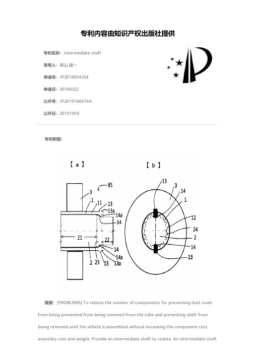
专利名称:Intermediate shaft发明人:森山 誠一申请号:JP2018054324申请日:20180322公开号:JP2019166874A公开日:20191003专利内容由知识产权出版社提供专利附图:摘要:[PROBLEMS] To reduce the number of components for preventing dust cover from being prevented from being removed from the tube and preventing shaft from being removed until the vehicle is assembled without increasing the component cost,assembly cost and weight. Provide an intermediate shaft to realize. An intermediate shaftwith a dust cover arranged in a state of being inserted through a through hole provided in a dash panel of a vehicle includes a columnar shaft portion having a male groove on the outer periphery, and a shaft portion of the shaft portion. Cylindrical tube 1 having a female groove 12 on the inner periphery thereof that externally fits male groove 24, and an annular shape that is fitted on tube 1 to close the gap between the outer peripheral surface of intermediate shaft 85 and the inner peripheral surface of the through hole. The first protrusion 13 that prevents the dust cover 3 from coming out of the tube 1 and the shaft 2 come out from the tube 1 at one end in the axial direction of the tube 1. And a second protrusion 14 for preventing the above. [Selection] Figure 4申请人:日本精工株式会社地址:東京都品川区大崎1丁目6番3号国籍:JP更多信息请下载全文后查看。
- 1、下载文档前请自行甄别文档内容的完整性,平台不提供额外的编辑、内容补充、找答案等附加服务。
- 2、"仅部分预览"的文档,不可在线预览部分如存在完整性等问题,可反馈申请退款(可完整预览的文档不适用该条件!)。
- 3、如文档侵犯您的权益,请联系客服反馈,我们会尽快为您处理(人工客服工作时间:9:00-18:30)。
THE INTERMEDIATE SHAFT COMPONENT
–DESIGN OF SHAFT, BEARINGS, KEYS, ETC
Group Name : Group number: Major Professor: Dr.Ni Feng
F F
x
0 0
x
Fbx Ax Fr Bx 0 Fbz Az Ft Bz 0 Az 80 Ft 230 Bz 380 0 Ax 80 M a Fr 230 Bx 380 0
z
M M
0 0
Group Member:
Completing Time: 12.08.2015
-1-
THE INTERMEDIATE SHAFT COMPONENT
01 Abstract: In this project, we have designed two different bearings,
a shaft, two different keys, two shaft sleeves, two bearing caps and some lip seals.In addition, all the positioning and fastening features needed for all the mounted elements and some other design details like pins and grooves have also been taken into considerations. We have made
-4-
THE INTERMEDIATE SHAFT COMPONENT
03 Introduction: The intermediate shaft supported by two bearings
and transmitting power from the belt pulley at the left end to the gear pinion in the middle of the shaft is to be designed. What’s more, all the positioning and fastening features needed for all the mounted elements and all the details, such as fasteners, threads, grooves, holes, etc on the shaft, also need to be taken into consideration. Some tables and diagrams are also required to better show our design. The key of the whole design is to minimize our cost as much as possible.
specific calculation to determine the accurate sizes of every part. A schematic assembly drawing and drawings of main parts are used to show the sizes of the relevant parts and their relative positions. Moreover, when we have determined a specific dimension, we choose to check FOS of every dimension to see whether our design is safe. If not, a new dimension is determined. Another goal we have achieved is to minimize
The left hand helical gear pinion: width wgear 35mm , normal module mn 3mm , normal pressure angle n 20 , helical angle 25.09 , N = 32 teeth .
features needed for all the mounATE SHAFT COMPONENT
B) Design the shaft for strength. C)Check shaft stiffness using estimation (deflections at key points) against some criteria for the mounted elements (bearings/gear). D)Determine suitable bearings for the loadings. E)Consider the shaft mounting in casing and select proper lip seals accordingly. F)Design keys wherever needed G)Finalise all the details, such as fasteners, threads, grooves, holes, etc on the shaft. H)Produce an engineering part drawing for the shaft, including all the tolerances and manufacturing requirements. I)Document the design in a design report, including a diagram showing the whole assembly (assembly drawings are not required).
mt mn cos 3 cos 25.09 2.717 mm Dgear mt N 2.71732 86.94mm P 10.6 KW n 1336 rpm T 9549 P 10.6 9549 75.76 N m n 1336
-5-
Above all, all the force and moment is
Fbx 625 N Fbz 1083 N
,
Ax 1260 N Az 500 N , A 816 N y
Fr 700 N F 1743 N t F a 816 N , M 75.8 N m t M a 35.5 N m
4.2 Bearing design
-8-
THE INTERMEDIATE SHAFT COMPONENT
THE INTERMEDIATE SHAFT COMPONENT
Ft 2T 275.76 1743 N Dgear 86.94 10 3
Fr Ft tan t Ft
tan n tan 20 1743 700 N cos cos 25.09
Fa Ft tan 1743 tan 25.09 816 N Dgear M t Ft 2 Dgear M a Fa 2 86.94 3 1743 2 75.8 N m 75.8 10 N mm 86.94 3 816 2 35.5 N m 35.5 10 N mm
04 Text
4.1 Analysis of force and moment
Total belt tension Fb 1250 N in the direction shown 30 from vertical.
Fx Fb sin 30 625 N Fx Fb cos 30 1083 N
Bx 65 N Bz 1160 N
-6-
THE INTERMEDIATE SHAFT COMPONENT
Generate the force diagrams and shear-moment diagrams.
-7-
THE INTERMEDIATE SHAFT COMPONENT
wgear 35mm , normal
n 20 , helical angle
25.09 , N 32 teeth .
6. Some of the formulae available are:
Ft 2 T / D gear mt mn cos , Fr Ft tan t Dgear mt N ,
z
625 Ax 700 Bx 0 1083 Az 1743 Bz 0 Az 80 1743230 Bz 380 0 Ax 80 35.5 103 700230 Bx 380 0 Ax 1260 N Bx 65.4 N Az 500 N Bz 1160 N
(horizontal,
radial),
(vertical,
radial), Fa Ft tan (horizontal, axial to the left), tan t cos tan n . 7. Assuming the bearing at the left end takes all the axial load. 8. The life required for the bearings is 15000 hours. The design tasks involve A) Sketch the intermediate shaft in terms of physical lengths and diameters for the functions including all the positioning and fastening