装载机前端工作机构建模及仿真
基于Pro/E的挖掘机虚拟样机建模及运动学仿真

图1
虚 拟 样 机 及 伺 服 电机 定 义
圈
收 稿 日期 :0 2 0 — 8 2 1— 4 0
作者简 介 : 徐素霞 (9 8 ) 女 , 18 一 , 内蒙古乌海人 , 学生 , 硕士研究 生 , 研究方向 ቤተ መጻሕፍቲ ባይዱ 研究方 向为机构 学与机械动力学 。 2 2 8
《 装备制造技术}0 2 2 1 年第 7 期
杆正转 到一定位置 , 铲斗正转进行挖掘作业 , 待铲斗 图2 是挖掘机 中间齿尖在 WC S坐标系关于 时问的 满载后 , 动臂反转 , 使铲斗抬升。同时斗杆和铲斗正 位 置 、 度 、 速 加速 度 图像 。 转调 整 姿 势 防止 洒 土 。然后 转 台反 转 至卸载 位置 , 斗
挖掘机是我 国经济建设中非常重要 的工程机械 之一 。因此 , 挖 掘机 机械 结构 和工 作过程 做深 入研 对 究 , 非 常 必要 的 。Po 是 rE是 一 款全 方 位 的三 维 产 品 / 开发软件 , 整合 了零件设计 、 品组装 、 产 工程制图、 造 型设计 、 机构设计 / 分析与动态仿真等各种功能。借 于 此技 术 , 工程 设 计 人 员 可 以在 制造 物理 样 机 之前 , 建立 虚 拟样 机模 型 , 拟实 际工 况进 行运 动仿 真 。根 模 据仿 真结 果 , 各 种 设计 方 案 进行 对 比 , 而确 定关 对 从 键 的设 计 参 数 , 预测 产 品 的机 械 性 能 , 以减 少产 品开 发周期 , 节省设计费用 , 提高产品品质及性能。 本文以某种挖掘机为样机 , 利用 Po rE建立虚拟 / 样机模 型 , 并对其进行运动仿真分析 , 通过数据分析 来 研究 挖 掘机 的工作 状况 。
1 挖掘机虚拟样机 的建模
多功能装载机工作装置机械-液压系统联合仿真
0 引 言
多功 能装 载 机 以其 优 异 的 机 动 性 能 和 工 况 适 应 性, 几乎 应用 于所有 的小规 模 土方 工 程 , 一种典 型 的 是 变 负载 、 多工况 的机 电液一 体化 产 品 。传统 的基 于
中 图分 类 号 :H 4 ;H 2 ; H 3 T 2 3 T 13 T 17 文 献 标 志 码 : A 文 章编 号 :0 1 4 5 (0 0 1 0 2 0 10 — 5 1 2 1 )2— 07— 5
Co b n d sm u a i n o e h n s - y a lc y t m f m i e i l t f m c a im h dr u is s s e o o wo k n e i e o u t-u c i n lwhe ll a e r i g d v c fm lif n to a e o d r
Abs r c t a t:I r e oa l z v me tprc s ft e wo k n e ie o lif ncina e lla e n o c lu ae te la fe ey p r , n o d rt nay e mo e n o e so h r i g d vc fmut—u to lwh e o d ra d t ac l t h o d o v r a t De a i— re eg meh d wa p le o e t b ih te k n ma iso c a s m o e ,a d i ut n o sy te d na ismo lo y r ui n vtHa tnb r to sa p id t sa ls h i e tc fme h nim d l n sm la e u l h y m c de fh d a lc
挖掘装载机工作装置结构设计论文
目录第一部分:系统开发建议书..........................共5页第二部分:WZ45.40装载工作装置设计.. (40)摘要:第一章:整机概述 (1)第一节:绪论 (1)第二节:国内外发展现状 (2)第三节:挖掘装载机发展特点 (5)第二章:铲斗设计······································.7 第三章:挖掘装载机工作装置结构设计·····················.10一、确定动臂长度、形状与车架的铰接位置 (11)二、连杆机构设计·······································.15三、转斗油缸与摇臂的铰接点以及下拉杆与机架铰接点的确定” (16)四、举升油缸与动臂和机架的铰接点 (17)五、铲斗举升平动分析及最大卸载高度、最小卸载距离的确定.................................................l 8 第四章:工作装置的受力分析............................21 第五章:工作装置的运动仿真. (32)第六章:工艺分析......................................33 第七章:工作装置的限位机构..............................35 第八章:设计心得及实习体会.............................37 第九章:附录............................................38 第三部分:翻译材料 (13)页系统开发建议书1.产品用途及使用范围:轮式装载机是一种用途广泛的施工机械,广泛应用于建筑公路铁路水电港口矿山及国防工程中,对加快工程建设速度减轻劳动强度提高工程质量降低工程成本都发挥这重要作用。
机械工程师如何进行机械运动仿真

机械工程师如何进行机械运动仿真机械运动仿真是现代机械工程领域的重要工具,它可以模拟和预测机械系统的运动轨迹和性能。
在设计和优化机械系统时,机械工程师可以通过运动仿真来评估不同设计方案的优劣,提高系统效率和性能。
本文将介绍机械工程师如何进行机械运动仿真。
第一步是建立模型。
机械运动仿真的第一步是建立准确的机械模型。
机械工程师需要根据实际的机械系统特性和约束,使用专业的仿真软件建立系统的数学模型。
这个模型包括机械系统的结构、零件的参数和运动学关系等。
通过建立准确的模型,机械工程师可以更好地理解和分析系统的运动行为。
第二步是选择仿真工具。
市面上有许多专业的机械运动仿真软件,机械工程师需要根据具体需求选择合适的工具。
一般而言,仿真软件应具备良好的计算精度、友好的用户界面和灵活的功能。
此外,还需注意软件是否支持导入和导出不同格式的模型文件,以便与其他设计和分析软件进行集成。
第三步是进行仿真分析。
在对机械系统进行仿真之前,机械工程师需要定义仿真参数和约束条件。
这些参数可以包括零件的材料特性、力和力矩的大小、摩擦系数等。
通过调整这些参数,机械工程师可以模拟不同工况下的机械系统行为。
同时,还需要考虑系统的约束条件,比如固定约束、转动约束等。
这些约束条件可以限制某些部件的运动自由度,使仿真结果更接近实际情况。
第四步是分析仿真结果。
仿真分析完成后,机械工程师需要对仿真结果进行详细的分析。
他们可以根据仿真结果评估机械系统的性能指标,如速度、加速度、力矩等。
此外,还可以分析零件的位移、变形和应力分布等。
通过分析仿真结果,机械工程师可以发现系统存在的问题,并进行必要的优化和改进。
最后一步是优化设计。
基于对仿真结果的分析,机械工程师可以进行优化设计。
他们可以通过改变零件的尺寸、材料或设计参数来改善系统性能。
优化设计通常采用试错法,即通过多次仿真分析和优化设计迭代,逐步优化机械系统的性能指标。
通过这样的优化过程,机械工程师可以设计出更加高效、稳定和可靠的机械系统。
基于ANSYS的装载机前车架结构的有限元分析
《装备制造技术》2018年第02期0引言装载机前车架与装配在其上的其余部件形成配合,是工作装置的基础部件,前车架的强度、刚度决定着整个机械的使用性能[1]。
本论文使用有限元分析软件ANSYS 对某装载机前车架作静力分析,获得在各典型工况下的整体应力应变分布情况。
这样就为装载机前车架的设计提供理论支持,达到了缩短设计周期、尽量增加经济效益的目的。
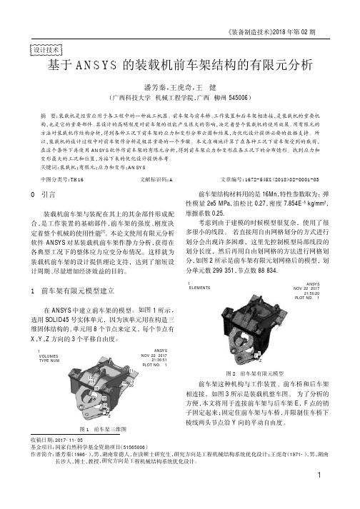
1前车架有限元模型建立在ANSYS 中建立前车架的模型。
如图1所示,选用SOLID45号实体单元,因为该单元用在构造三维固体结构的。
单元用8个节点来定义,每个节点有X ,Y ,Z 方向的3个平移自由度。
前车架结构材料用的是16Mn ,特性参数取为:弹性模量2e5MPa ,泊松比0.27,密度7.854E -6kg/mm 3,摩擦系数0.25.考虑到由于建模的时候模型很复杂,使用了很多很小的线段。
若直接用自由网格划分的方式进行划分会出现许多困难,这里先控制模型局部线段的划分长度,然后再用自由划网格的方法进行网格划分,如图2所示是前车架有限元划网格后的模型,划分单元数299351,节点数88834.前车架这种机构与工作装置、前车桥和后车架相连接,如图3所示是装载机整车图。
为了分析的方便,本文将用于连接前车架与后车架E ,F 点的销子固定起来;固定住前车架与车桥,并限制住车桥下棱线两头节点沿Y 向的平动自由度。
基于A N S Y S 的装载机前车架结构的有限元分析潘芳秦,王虎奇,王健(广西科技大学机械工程学院,广西柳州545006)摘要:装载机是经常应用于各工程中的一种施工机器。
前车架与前车桥、工作装置和后车架相连接,是装载机的重要机构,也是它的重要部件。
其设计的高明程度对前车架的性能产生很大的影响,决定着整个装载机的使用效果。
用有限元的方法对装载机作结构分析,得到各种工况下前车架的应力和变形分布云图和结果,为优化设计提供必要的数据支持。
所以,装载机的设计过程中对前车架作分析是极其重要的一个步骤。
装载机铲装装置的虚拟装配和运动仿真研究

FU ̄ AN NO NGJI
装载机铲装装置 的虚拟装配和运 动仿真研究
吴 玉 荣
( 田 市 荣兴 机 械 有 限公 司 , 建 莆 田 3 1 0 ) 莆 福 5 10
摘 要 : 章介 绍 了 P o E g e 件在 装载机 铲装 机构 设 计分析 中的应用 。通过 对机构 建立合 理 的 文 /n1 e r n r软
产 品参 数化 设 计 、 动 校 核及 运 动 力 学等 分 析 , 过 运 通 其 快速 、 观 的建 模 , 分显 示 出 各部 件 运 动 中相 互 直 充
间的协调 关 , 又可 用来检 验 设计过 程 的合理 性和 正
确性 。
1 铲 装 装 置 的 建 模 及 虚 拟 装 配
速 发展 , 成为 工程机 械 的主要 机种 之一 。 目前 装载 机 市场 上 出现一 些 有特 殊 构造 、有特 色 的和 多 功 能产
品, 这种 发展趋 势 既体现 各 厂家市场 差 异化 的产 品战 略, 又体 现各 自的技术水 平和 实力 。这 些变 化对 产 品 的设计手 段和 设计 效率 提 出 了更 高 的要求 。
以确 定 , 重复工 作量 大 。 了解 决这 些 问题 , 公司采 为 本
实现 。随 着计算 机辅 助设 计技 术 的发展 , 借助 目前 最
流行 的三 维设计 软件 之一 P o E g n e r / n i e r软件 ,进行
用 了 P o E g e r / n e r软件对 该铲 装装 置进行 仿真和 分 i n 析 , 拟 它在真 实环 境 的工作状 况 并获取 其主要 机构 模 的受力 分析 , 以及 早发现 设计缺 陷, 缩短 设计周 期 。
基于AMESim的小型挖掘机执行机构液压系统建模与仿真解读

第26卷第4期青岛大学学报(工程技术版)Vol.26No.42011年12月JOURNALOFQINGDAOUNIVERSITY(E&T)Dec.2011文章编号:10069798(2011)04004305基于AMESim的小型挖掘机执行机构液压系统建模与仿真刘震,王玉林,张鲁邹,尹彦章,公丕权(青岛大学机电工程学院,山东青岛266071)摘要:为提高国内挖掘机液压技术水平,以某型号小型挖掘机为例,基于AMESim对包括动臂、斗杆、铲斗在内的小型挖掘机执行机构的液压系统进行了建模,修正了以往研究者在建造此类模型时主换向阀的阀芯反向移动时,弹簧反馈力加倍的错误。
仿真并分析了无负载情况下执行机构的单独动作与复合动作的特性。
仿真结果与理论分析吻合,为挖掘机液压系统的研究提供了重要参考。
关键词:液压挖掘机;AMESim;执行机构;模型;仿真中图分类号:TP391.92;S222.5+6文献标识码:A收稿日期:2011-09-26作者简介:刘震(1986-),男,山东临沂人,硕士研究生,主要研究方向为现代设计方法与制造技术。
挖掘机是用来开挖土壤的施工机械,它在减轻繁重的体力劳动,保证工程质量,加快建设速度以及提高劳动生产率方面起着十分重要的作用。
在农田水利、建筑工程、能源交通建设以及现代化军事工程等领域得到了广泛的应用[]。
目前作为一种万能型工程机械,挖掘机已经成为工程机械的第一主力机种,在世界工程机械市场上已据首位,并且仍在发展扩大[3]。
然而,国内挖掘机液压技术研发水平一直远远落后于国外。
虽然国内一些挖掘机生产厂通过采取与国外合资、积极引进国外先进的液压元件等措施,使国内生产的一些挖掘机技术水平得到迅速提高,但也存在购买国外液压部件成本高,产量受限,维修、匹配困难等问题。
而且在最新技术上与国外相比还存在较大差距。
近年来,由于计算机仿真技术在科学研究中的应用,它不仅缩短了研发周期,降低成本,也减少了很多人为因素。
ZL50G-7装载机驱动桥设计与三维建模

半轴设计
在一般非断开式驱动桥上,驱动车轮的传 动装置就是半轴,这时半轴将差速器半轴齿轮 与轮毂连接起来。 半轴的型式我选用的是全浮式半轴,对半 轴的设计计算均是按全浮式半轴进行的,具体 请参见说明书。
20112011-8-22
轮边减速器设计
在装载机上使用轮边减速器,它可以使主 传动减速器的速比适当减小,多采用单排行星 齿轮传动,太阳轮与半轴通过花键连接,齿圈 与轮毂固定安装,我选用4 与轮毂固定安装,我选用4个行星轮安装。其 具体计算请参见设计说明书。
20112011-8-22
主减速器建模
主减速器建模零件有:叉形凸缘、油封 座、主动锥齿轮前轴承座、槽形扁螺母、 主动锥齿轮、主减速器壳、主动锥齿轮前 轴承、油封座垫圈、主动锥齿轮后轴承、 垫圈、隔套、主减速器壳垫片、主减速器 轴承盖、主减速器轴承盖螺栓。
主减速器主要部件建模展示
20112011-8-22
20112011-8-22
桥壳设计
桥壳用以承受传力,承受垂直载荷,并 将作用于轮上的牵引力,并将作用于轮上 的牵引力,制动力,横向力等传给车架, 装载机作业时,桥壳受力情况复杂,设计 时必须使其具有足够的强度、刚度 ,本设 计中驱动桥我采用整体式桥壳 。 桥壳的强度计算主要是对应力的计算, 详细计算请参见说明书。
齿圈
齿 圈 座
轮 边 减 速 器 壳 行星
20112011-8-22
行星
半 轴
20112011-8-22
桥壳
20112011-8-22
主减速器装配
20112011-8-22
差速器装配
20112011-8-22
轮边减速器装配
20112011-8-22
驱动桥总体装配
- 1、下载文档前请自行甄别文档内容的完整性,平台不提供额外的编辑、内容补充、找答案等附加服务。
- 2、"仅部分预览"的文档,不可在线预览部分如存在完整性等问题,可反馈申请退款(可完整预览的文档不适用该条件!)。
- 3、如文档侵犯您的权益,请联系客服反馈,我们会尽快为您处理(人工客服工作时间:9:00-18:30)。
ORIGINAL ARTICLECompound mechanism modeling of wheel loaderfront-end kinematics for advance engineering simulationYing Li &Wenyuan liu &Samuel FrimpongReceived:23September 2014/Accepted:23November 2014/Published online:6December 2014#Springer-Verlag London 2014Abstract Compound closed-loop mechanism methodology is proposed to model the wheel loader front-end kinematics for simulating the mechanism motion in a dynamic environ-ment.For the numerical modeling purpose,the mechanism is considered as consisting of three vector loops connected by the joint angles or displacements.Each vector loop is formu-lated as time-dependent ordinary differential equations (ODEs).The simulations cover the numerical solutions of the forward and reverse kinematics differential equations.The consistency error check approach is employed to validate the simulation.A case study is presented to demonstrate the reverse kinematics simulation of the compound mechanism model in Simulink environment,which includes the user-defined program,numerical solution,and error analysis.The displacement-time variations of two driving cylinders are obtained with the inputs of the lift and rotation bucket accel-erations.The simulation is validated with the numerical anal-ysis of the error results.This research provides a significant method to simulate the wheel loader motion for wide-ranging engineering application.Keywords Wheel loader .Compound mechanism modeling .Closed vector loop .Kinematics simulation .Error analysis1IntroductionThe wheel loaders are the heavy mining and construc-tion equipment,which function as loading,lifting,transporting,and discharging materials as displayed in Fig.1a –d ,respectively.Figure 2illustrates the main structural components of the wheel loader front-end attachment.It has a front-mounted bucket and a link-age controlled by two mechanisms:one is the lift mechanism (links 1–3)driven the hydraulic cylinder 3for lifting arm 4,and the other is the rotation mecha-nism (links 8–15)driven by hydraulic cylinder 8for rotating bucket 7[1].Kinematics model of wheel loader allows engineers to design dynamics control system to achieve the operation automation,and kine-matics simulation of wheel loader allows engineers to examine dynamic machine performance to achieve the design optimization.The detailed literature survey of the modeling and simulation of the mining equipment front-end attach-ment is presented in our previous publications [2–4].The kinematics modeling methods regarding the front-end attachments of mining equipment are focused on the closed or open kinematics loop [2–8].The closed-loop modeling method based on the theory of machin-ery kinematics [9]is applied to the kinematics modeling of the simple mechanism with four or less links.The open-loop modeling method based on the theory of robot kinematics [10]is applied to the kinematics modeling of the complicated mechanism with five or more links.The simulation methods are condensed on the forward and reverse kinematics simulation.The for-ward simulation is to find a trajectory of the bucket for the given motions (displacements,velocities,and accel-erations)of driving links,whereas the reverse simula-tion is to solve the required displacements,velocities,Y .Li (*)North University of China,Taiyuan,Shanxi,China 030051e-mail:liyinglzh@W.liuUniversity of Texas-UTMB,Galveston,TX,USA S.FrimpongUniversity of Missouri-Rolla,Rolla,MO,USAInt J Adv Manuf Technol (2015)78:341–349DOI 10.1007/s00170-014-6640-7and accelerations of the driving links for a given tra-jectory of the bucket.A typical wheel loader consists of multi-links as described in Fig.2,and the linkage motions are intertwined with other links as indicated in Fig.1.In our recent academic research [3],a wheel loader front-end is modeled as a seven-bar mechanical manipulator via open-loop concepts.The forward kinematics method is employed to formulate the kinematics equations in Cartesian coordinates for kinematics simulation.This model is the graduate student level understanding of kinematics and may not be accepted by all engineers.For the research purpose,a novel closed kinematics loop model of the cable shovel is developed based on kinematics of machinery in our lab [2].The kinematics model of the cable shovel is modeled as a seven-bar linkage with four degrees of freedom,which comprises the upper attachment and the dumping mechanisms.The motion equation of each mechanism is given by attaching Cartesian coordinates to schematic diagram of the kinematics model.A virtual prototype of the cable shovel is built,which allows the visualization of(a) Loading (b) LiftingFig.1A typical operation process of wheelloaderFig.2Main structure components of a wheel loader front-end attachment.1front vehicle body,2crank 3lift cylinder,4lift arm,5arm link,6bellcrank,7bucket,8bucket cylinder,9rotating link,10crank,11frame,12rotating link,13connecting rod,14crank,and 15framea three-dimensional motion of general mechanical sys-tem and the prediction of interference among the struc-tural components of the cable shovel.The numerical results of displacement,velocity,and acceleration can be used to evaluate the kinematics performance of cable shovel for its optimization.This study provides a solid foundation for further kinematics modeling and simula-tion of wheel loader in the engineering applications.For the engineering application purpose,the closed kinematics loop models,which are developed base on undergraduate student course [1,11],are proposed to simulate wheel loader motions.However,there are mas-sive links in the front-end attachment,so the link kine-matics model cannot be established in one closed loop.This study outlines the compound closed-loop mecha-nisms method,which can allow engineers to develop the wheel loader kinematics model with multi-simple mechanisms.The research include the following:first,the wheel loader front-end is modeled as a compound mechanism with three simple mechanisms;second,the vector loop equations of each mechanism are developed according to the geometric relations among the machinery links;third,the forward and reverse kinematics simulations are described;and fourth,an example is presented for demonstrating the method applications.2Kinematics modeling of the front-end compound mechanismFigures 3,4,and 5show the vector loop schematic diagrams of the wheel loader front-end attachment with local coordinate systems.The front-end attachment is regarded as a compound mechanism including a lift mechanism (slider-crank mechanism)with links 1–3and a rotation mechanism,which consists of a slider-crank mechanism with links 8–11and a four-bar mecha-nism with links 12–15.These three mechanisms form three vector loops 1–3,respectively [1].If each vector loop has N links and each link can associate a vector,the magnitude of this vector r i is the length of the link,whereas the direction of this vector is along the link.i and r i are the velocity and acceleration of link i ,respectively.The angle θi is defined as counterclockwise positive from the positive x -direction and drawn to the tail of each vector.ωi and αi are defined as the angular velocity and acceleration for link i ,respectively.The mathematical representation for each vector loop is given as Eq.1,where the sum of all vectors in the loop must be equal to zero [11].X i ¼1N r i ¼0ð1ÞIf each vector can be represented in Eq.2,Eq.1can be written as the loop-closure Eq.3.r i ¼r i cos θi ;sin θiÀÁTð2ÞX i ¼1N r i ¼X i ¼1N r i cos θi ;sin θi ðÞT ¼0ð3ÞThe loop-closure equations of each loop are established as follows.Figure 3displays a vector loop 1diagram of the slider-crank mechanism,which is attached to the front vehicle body by two revolute joints O 1and O 2.The local coordinate system O 2(X 2,Y 2,Z 2)is affixed to the link 1at joint O 2with the X 2axis along O 2O 1.The lift motion of the bucket can be obtained by hydraulic cylinder (link 3)rotating lift arm.The frame is link 1,the crank is link 2,and the connecting rod is link 3.Equation 3can be written as x and y coordinates (Eqs.4–5).r i cos θ1þr 2cos θ2þr 3cos θ3¼0ð4Þr 1sin θ1þr 2sin θ2þr 3sin θ3¼0ð5ÞThe velocity matrix Eq.6can be derived by taking the firsttime derivative of Eqs.4–5.−r 3sin θ3cos θ3r 3cos θ3sin θ3 !ω3r 3!¼r 2ω2sin θ2−r 2ω2cos θ2 !ð6ÞThe acceleration matrix Eq.7can be obtained by taking the second derivative of Eqs.4–5.−r 3sin θ3cos θ3r 3cos θ3sin θ3!α3r 3!¼2r 3ωsin θ3þr 3ω23cos θ3þr 2α2sin θ2þr 2ω22cos θ2−2r 3ω3cos θ3þr 3ω23sin θ3−r 2α2cos θ2þr 2ω12sin θ2"#ð7ÞFigure 4illustrates a vector loop 2diagram of the slider-crank mechanism,which is attached to the front vehicle bodyby two revolute joints O 2and O 3.The local coordinate system O 3(X 3,Y 3,Z 3)is assigned to the link 11at point O 3,with the X 3axis along O 3O 2.The link 9motion can be given by hydraulic cylinder (link 8)and lift arm (link 10).The frame is link 11,the cranks are links 9and 10,and the connecting rod is link 8.Equation 3can be broken down into x and y coordinates (Eqs.8–9).r 8cos θ8þr 9cos θ9þr 10cos θ10þr 11cos θ11¼0ð8Þr 8sin θ8þr 9sin θ9þr 10sin θ10þr 11sin θ11¼0ð9ÞThe velocity matrix Eq.10can be derived by taking the first derivative of Eqs.8–9for loop 2.−r 8sin θ8cos θ8r 8cos θ8sin θ8!ω8r 8!¼r 9ω9sin θ9þr 10ω10sin θ10r 9ω9cos θ9−r 10ω10cos θ10!ð10ÞThe acceleration matrix Eq.11can be given by taking the second derivative of Eqs.8–9.−r 8sin θ8cos θ8r 8cos θ8sin θ8!α8r 8!¼2r 8ω8sin θ8þr 8ω28cos θ8þr 9ω29cos θ9þr 9α9sin θ9þr 10ω210cos θ10þr 10α10sin θ10−2r 8ω8cos θ8þr 8ω28sin θ8þr 9ω29sin θ9−r 9α9cos θ9þr 10ω210sin θ10−r 10α10cos θ10"#ð11ÞFigure 5indicates a vector loop 3diagram of the four-barmechanism,which is attached to the lift arm by two revolute joints O 4and O 5.The local coordinate system O 4(X 4,Y 4,Z 4)is assigned to the lift arm at joint O 4,with the X 4axis along O 4O 5.The rotating motion of the bucket can be generated by rotating link 9.The rotating motion of the bucket can be generated by rotating link 12.The dynamic frame is link 15,the cranks are links 12and 14,and the connecting rod is link 13.Equation 3can become x and y coordinates (Eqs.12–13).r 13cos θ13þr 14cos θ14þr 12cos θ12þr 15cos θ15¼0ð12Þr 13sin θ13þr 14sin θ14þr 12sin θ12þr 15sin θ15¼0ð13ÞThe matrix velocity Eq.14can be derived by taking the first time derivative of Eqs.12–13for loop 3.r 12sin θ12r 13sin θ13r 12cos θ12r 13cos θ13 !ω12ω13 !−r 14ω14sin θ14−r 14ω14cos θ14!ð14ÞThe acceleration matrix can be expressed as Eq.15by taking the second derivative of Eqs.12–13.local coordinatesystemFig.4Vector loop 2diagram of the slider-crank mechanism with local coordinate systemr12sinθ12r13sinθ13 r12cosθ12r13cosθ13!α12α13!¼−r13ω213cosθ13−r14α14sinθ14−r14ω214sinθ14−r12ω212cosθ12r13ω213sinθ13−r14α14cosθ14þr14ω214sinθ12þr12ω212sinθ12!ð15ÞThree loop equations are combined in the assembled form through mathematical relationships to capture the front-end system motion characteristics.Therefore,the combined math-ematical model is developed as time-dependent ordinary dif-ferential equations(ODEs)and ready to be solved numerically in kinematics simulation.3Kinematics simulation of the front-end compound mechanismFigure6describes a schematic diagram of compound mech-anism used for the kinematics simulation of the wheel loader front-end attachment.Two problems of forward kinematics and inverse kinematics are solved as discussed below. Forward kinematics simulation For the given displacement-time variables of the two hydraulic cylinders,r3(t)and r8(t), the bucket position-time variables,θ2andθ14,are yielded by the solutions of Eqs.4,5,8,9,12,and13through loops1–3.&In loop1,the slider-crank mechanism initial position is defined by the link lengths of r1,r2,and r3=r3(0)and angles ofθ1,θ2=θ2(0),andθ3=θ3(0).For a given input displacement of the hydraulic cylinder(link3),r3=r3(t), the two link angles ofθ2andθ3,are found by solving Eqs.4–5.&In loop2,the slider-crank mechanism initial position is defined by the link lengths of r8=r8(0),r9,r10,and r11and angles ofθ8=θ8(0),θ9=θ9(0),θ10=θ10(0),andθ11.One of the solutions of Eqs.4–5,θ2,becomes one of inputsθ10 into loop2.When other one is the displacement of thehydraulic cylinder(link8),r8=r8(t),the solution of Eqs.8–9produces the link9motionθ9.&In loop3,the four-bar mechanism initial position is de-fined by the link lengths of r12,r13,r14,and r15and angles ofθ12=θ12(0),θ13=θ13(0),θ14=θ14(0),andθ15.When the solutions from the loops1and2,θ15(θ2),andθ12(θ9), are used as inputs,θ13andθ14are given by solving Eqs.12–13.Therefore,it needs two independent input motions to op-erate the bucket.This means the displacements r3(t)and r8(t) have to be provided by the two hydraulic cylinders3and8 (see Fig.2),respectively.Reverse kinematics simulation For the given position-time variables of the bucket,θ2andθ14,the displacement-time variables of two hydraulic cylinders,r3(t)and r8(t),are yielded by the solutions of equations from15to4through loop3to loop1.&In loop3,the four-bar mechanism initial position is de-fined by the link lengths r12,r13,r14,and r15and angles of θ12=θ12(0),θ13=θ13(0),θ14=θ14(0),andθ15.If the motion of bucket,θ13andθ14,is given,the angular displacementsθ12(θ9)andθ15(θ2)are yielded by solving Eqs.12–13.The solutions of Eqs.14–15product the angular velocitiesω12(ω9)andω15(ω2),andα12(α9)accel-eration andα15(α2),respectively.&In loop2,the slider-crank mechanism initial position is defined by the link lengths of r8=r8(0),r9,r10,and r11, and angles ofθ8=θ8(0),θ9=θ9(0),θ10=θ10(0),andθ11.As the solutions from loop3,θ9andθ10(θ2),are asinputs, coordinate systemthe solutions of Eqs.8–11product the hydraulic cylinder (link 8)displacement r 8,velocity 8,and acceleration r 8,respectively.&In loop 1,the slider-crank mechanism initial position is defined by the link lengths r 1,r 2,and r 3=r 3(0)and angles of θ1,θ2=θ2(0),and θ3=θ3(0).When the solutions from loop 3,θ2,becomes an input into loop 1,the solutions of Eqs.4–7product the hydraulic cylinder (link 3)displace-ment r 3,velocity 3,and acceleration r 8,respectively.Therefore,it needs two independent bucket motion param-eters to solve the compound mechanism driving variables,which is provided by the two hydraulic cylinders 3and 8(see Fig.2),respectively.4Simulation validation of the front-end compound mechanismThe kinematics simulation of the front-end compound mech-anism described in “section 3”is validated using the consis-tency check approach [11].No matter what kind of simulation it is,the inputs for the forward kinematics or the reverse kinematics simulations are the motion parameters of the two input links;the remaining velocities and accelerations of the linkages are solved by deriving the vector loop equations;and then these variables are integrated to compute the displace-ments of two hydraulic cylinders,r 3and r 8,or the bucket positions,θ2and θ14.An error is defined as difference between the resulting position and original position as describedinFig.6Compound mechanism diagram of the wheel loader front-endattachmentFig.7Simulink diagram for kinematics simulation of wheel loader front-end compound mechanismEq.16.E ¼X i ¼1N r i ¼X i ¼1N r i cos θi ;r i sin θi ðÞTð16ÞFor loop 1,the error Eq.16can be expressed as x and y coordinates (Eqs.17–18).e x 1¼r 1cos θ1þr 2cos θ2þr 3cos θ3ð17Þe y 1¼r 1sin θ1þr 2sin θ2þr 3sin θ3ð18ÞFor loop 2,the error Eq.16can be described as x and y coordinates (Eqs.19–20).e x 2¼r 8cos θ8þr 9cos θ9þr 10cos θ10þr 11cos θ11ð19Þe y 2¼r 8sin θ8þr 9sin θ9þr 19sin θ10þr 11sin θ11ð20ÞFor loop3,the error Eq.16can be indicated as x and y coordinates (Eqs.21–22).e x 3¼r 13cos θ13þr 14cos θ14þr 12cos θ12þr 15cos θ15ð21Þe y 3¼r 13sin θ13þr 14sin θ14þr 12sin θ12þr 15sin 15ð22ÞThe norm of the three vector Eqs.16–22generates the root-mean-square error of the compound mechanism as showed in Eq.23.e ¼e 2x 1þe 2y 112þe 2x 2þe 2y 2 12þe 2x 3þe 2y 312ð23ÞOnce the acceptance tolerance limit is defined,the simula-tion error can be checked within the time ually,theerror tolerance is caused by the model structure and numerical solution in the coding program.If the numerical integration does not converge,lower the acceptance tolerance limit is suggested.If the error is within the acceptance allowance limit,the simulation is validated.5Case study of the front-end compound mechanism A case study is performed for indicating the reverse kinemat-ics modeling,simulation,and error check of the wheel loader front-end compound mechanism in the MATLAB/Simulink software environment.The simulation model is developed using Simulink blocks and user-defined program blocks.The simulation involves the numerical solution of the ODEs that describe the time-varying responses of the front-end compound mechanism.The displacement-time results of two driving cylinders are obtained with the inputs of the lift and rotation bucket motions.The dynamic simulation errors are examined by analyzing the error-time and error-cylinder relationships.Simulation model Figure 7illustrates a Simulink block dia-gram model used to simulate the motion of a wheel loader front-end compound mechanism.The model embodies three user-defined program blocks to solve a series of the time-dependent ODEs derived in vector loops 1–3.The numerical integration blocks are employed for calculating velocities and displacements by integrating accelerations.Gain block sums the consistency errors of three loop equations.Simulation configuration parameters are set as Runge-Kutta ODE Solver,automatic step-size control and 18-s run time.The appropriate kinematics parameters such as the link geometric properties and initial conditions are addressed in Table 1.The reverse kinematics simulation refers to five steps:(a)input the angular accelerations of the lift arm and rotation bucket,(b)repeatedly solve the three loop ODEs through time steps,(c)integrate the resultant accelerations and velocities at each iteration step,(d)output the displacement values of two hydraulic cylindersTable 1Structural kinematics parameters and initial conditionsLength (m)Angle (°)Loop 1r 1r 2r 3(0)θ1θ2(0)θ3(0)1.9940.925 2.177−18088.57334.86Loop 2r 8(0)r 9r 10r 11θ8(0)θ9(0)θ10(0)θ112.4 1.0 2.6090180−67.38−180Loop 3r 12r 13r 14r 15θ12(0)θ13(0)θ14(0)θ151.01.10.5211.25838.318−78.25461.347−180over simulation time,(e)and check the simulation root-mean-square errors to ensure accurate solutions.Simulation inputs Figure8shows that the simulation inputs during the operating time18s with9s for lifting and9s for rotating motions.Figure8a indicates the angular acceleration of the lift arm variation with time relative to the O2(X2,Y2,Z2) coordinate system(see Fig.3).The angular acceleration jumps from0to0.077rad/s2at the0th second,linearly decreases to −0.078rad/s2from0to9s,sharply returns to0rad/s2at the 9th second,and then stays at the constant0rad/s2from9to 18s.The minimum angular acceleration of−0.078rad/s2 occurs at the9th second while the maximum of0.077rad/s2 occurs at the0th second.Figure8b depicts the angular accel-eration of the rotation bucket variation with time relative to the O4(X4,Y4,Z4)coordinate system(see Fig.5).The angular acceleration keeps a constant0rad/s2during the first9s,rises from0to0.13rad/s2at the9th second,linearly decreases from 0.13to−0.13rad/s2with time during the last9s and then jumps back from−0.13to0rad/s2at the18th second.The minimum angular acceleration of−0.13rad/s2occurs at the 18th second while the maximum of0.13rad/s2occurs at the 9th second.These inputs indicate that the arm mechanism motion is performed during the first9s while the bucket rotating motion is performed during the last9s.Simulation results Figure9shows that the simulation outputs during the operating time18s with9s for lifting and9s for rotating motions.The displacement of the lift cylinder varia-tion with time relative to the O2(X2,Y2,Z2)coordinate system (see Fig.3)is given in Fig.9a.The displacement non-linearly increases from a minimum of2.18m at the beginning to a maximum of2.82m at9s,and then stays at a constant of 2.82m from9to18s.The displacement within the last time segment(9to18s)does not change with time because the lifting motion is completed at the end of the9th second. Figure9b depicts the displacement of the rotation bucket cylinder variation with time relative to the O4(X4,Y4,Z4) coordinate system(see Fig.5).The displacement keeps a constant maximum of2.4m during the first9s,non-linearly decreases from2.4m to a minimum of2.2m during9to14s, and non-linearly increases from2.2to2.25m during the last 4s.The displacement within the first time segment(0to9s) does not change with time,because the bucket rotating motion starts at the9th second.Two output results show that the cylinder displacements vary smoothly with time during the operation.Simulation validation Figure10indicates that the root-mean-square error check during the simulation time18s with9s for lifting and9s for rotating motions.Figure10a gives theerror Fig.9Two cylinder displacement outputs with time:a lift cylinder displacement and b rotation bucket cylinderdisplacementFig.8Two link angular acceleration inputs with time:a lift arm angular acceleration and b rotation bucket angular accelerationvariation with time and Fig.10b displays the error variation with displacements of the lift cylinder and rotation bucket cylinder.The results show that the simulation error is quiet small and nearly constant of6.19×10−3m over time.In this validation,the acceptance tolerance limit is suggested as 10−2m considering the geometric model error and initial condition measurement errors[3].The resulting error is ac-ceptable,which is less than10−2m.Therefore,the resulting the positions of two hydraulic cylinders satisfy the original three vector loop equations throughout simulation time.The reverse kinematics simulation of the front-end compound mechanism is validated.6ConclusionsCompound mechanism methodology has been proposed to model the wheel loader front-end kinematics for efficient engi-neering simulation.The front-end mechanism is decomposed into three simple mechanisms,which forms three closed kine-matics chains.The mathematical modeling technology of the closed vector loop is employed to derive kinematics ODEs for each simple mechanism.The three loops are related by the joint kinematics parameters of the angles or displacements between adjacent links.The forward and reverse kinematics is used to simulate the compound mechanism model by the numerical solutions of differential equations.The consistency check meth-od is applied to validate the simulation.An example is given to indicate the reverse kinematics simulation of the compound mechanism model in Simulink environment.The study involves the user-defined program, numerical integration,dynamic simulation,and error check. The position problems of two driving cylinders are solved with the inputs of the lift and rotation bucket accelerations. The result of error variation with time shows that the sum of three loop errors is about6.19×10−3m,which is less than the acceptance tolerance of10−2m.This research has provided a significant approach for engi-neers to analyze and optimize wheel loader front-end attach-ment motion.Three aspects require to be improved through further research investigation.They are as follows:(1)case study of forward kinematics simulation of wheel loader front-end compound mechanism,(2)kinematics modeling and sim-ulation of a full wheel loader using the compound mechanism closed-loop method,and(3)development of wheel loader dynamics control system to simulate dynamic wheel loader performance.References1.Vinogradov O(2000)Fundamentals of kinematics and dynamics ofmachines and mechanisms.CRC Press,New York2.Frimpong S,Li Y(2007)Spatial kinematics and virtual prototypesimulation of the cable shovel performance.Trans Soc Min Metall Explor322:78–873.Li Y,Liu WY(2013)Spatial kinematics modeling and simulation ofwheel loader.J Model Simul Identif Control1(2):78–884.Li Y,Liu WY(2014)Comparison of advanced dragline dynamicsmodels for efficient engineering analysis.Int J Adv Manuf Technol 72:757–764,No.5–85.Daneshmend L,Hendricks C,Wu S.and Scoble M(1993)Design ofa mining shovel simulator.Innovative Mine Design for the21stCentury.©A.A.Balkema;Kingston,Ontario,Canada:551–561 6.Hemami A(1994)Modeling,analysis and preliminary studies forautomatic scooping.Adv Robot8(5):511–5297.Koivo AJ(1992)Kinematics of excavators(backhoes)for transfer-ring surface material.J Aerosp Eng7(1):17–328.Takahashi H,Morikawa Y,Tateyama K,Fukagawa R(2004)Studyon the mechanism of over-head-type load-haul-dump with a vessel.J Terramech41:175–1859.Wilson CE,and Sadler JP(1991)Kinematics and dynamics ofmachinery,2nd Edition.©Harper Collins College,New York 10.Ho CY and Sriwattanathmma J(1989)Robot kinematics symbolicautomation and numerical synthesis.©Ablex Publishing Corporation,Norwood,New Jersey11.Gardner J(2001)Simulations of machines using Matlab andSimulink,1st Edition.Brooks/Cole,University ofCalifornia Fig.10Root-mean-square errors:a error with time18scones and b error with two hydraulic cylinder displacements。