ABAQUS_Standard用户材料子程序实例

合集下载

Abaqus User Subroutines Reference Guide 用户材料子程序帮助文档

1.1.41 UMATUser subroutine to define a material's mechanical behavior.Product: Abaqus/StandardWarning: The use of this subroutine generally requires considerable expertise. Y ou arecautioned that the implementation of any realistic constitutive model requires extensivedevelopment and testing. Initial testing on a single-element model with prescribedtraction loading is strongly recommended.References“User-defined mechanical material behavior,” Section 26.7.1 of the Abaqus Analysis User's Guide“User-defined thermal material behavior,” Section 26.7.2 of the Abaqus Analysis User's Guide*USER MA TERIAL“S D V I N I,” Section 4.1.11 of the Abaqus V erification Guide“U M A T and U H Y P E R,” Section 4.1.21 of the Abaqus V erification GuideOv erv iewUser subroutine U M A T:can be used to define the mechanical constitutive behavior of a material;will be called at all material calculation points of elements for which the material definition includes auser-defined material behavior;can be used with any procedure that includes mechanical behavior;can use solution-dependent state variables;must update the stresses and solution-dependent state variables to their values at the end of theincrement for which it is called;must provide the material Jacobian matrix, , for the mechanical constitutive model;can be used in conjunction with user subroutine U S D F L D to redefine any field variables before they are passed in; andis described further in “User-defined mechanical material behavior,” Section 26.7.1 of the AbaqusAnalysis User's Guide.Storage of stress and strain componentsIn the stress and strain arrays and in the matrices D D S D D E, D D S D D T, and D R P L D E, direct components are stored first, followed by shear components. There are N D I direct and N S H R engineering shear components. The order of the components is defined in “Conventions,” Section 1.2.2 of the Abaqus Analysis User's Guide. Since the number of active stress and strain components varies between element types, the routine must be coded toprovide for all element types with which it will be used.Defining local orientationsIf a local orientation (“Orientations,” Section 2.2.5 of the Abaqus Analysis User's Guide) is used at the same point as user subroutine U M A T, the stress and strain components will be in the local orientation; and, in the case of finite-strain analysis, the basis system in which stress and strain components are stored rotates with the material.StabilityY ou should ensure that the integration scheme coded in this routine is stable—no direct provision is made to include a stability limit in the time stepping scheme based on the calculations in U M A T.Convergence rateD D S D DE and—for coupled temperature-displacement and coupled thermal-electrical-structural analyses—D D S D D T, D R P L D E, and D R P L D T must be defined accurately if rapid convergence of the overall Newton scheme is to be achieved. In most cases the accuracy of this definition is the most important factor governing the convergence rate. Since nonsymmetric equation solution is as much as four times as expensive as the corresponding symmetric system, if the constitutive Jacobian (D D S D D E) is only slightly nonsymmetric (for example, a frictional material with a small friction angle), it may be less expensive computationally to use a symmetric approximation and accept a slower convergence rate.An incorrect definition of the material Jacobian affects only the convergence rate; the results (if obtained) are unaffected.Special considerations for various element typesThere are several special considerations that need to be noted.A v ailability of deformation gradientThe deformation gradient is available for solid (continuum) elements, membranes, and finite-strain shells(S3/S3R, S4, S4R, SAXs, and SAXAs). It is not available for beams or small-strain shells. It is stored as a 3× 3 matrix with component equivalence D F G R D0(I,J). For fully integrated first-order isoparametric elements (4-node quadrilaterals in two dimensions and 8-node hexahedra in three dimensions) the selectively reduced integration technique is used (also known as the technique). Thus, a modified deformation gradientis passed into user subroutine U M A T. For more details, see “Solid isoparametric quadrilaterals and hexahedra,”Section 3.2.4 of the Abaqus Theory Guide.Beams and shells that calculate transv erse shear energyIf user subroutine U M A T is used to describe the material of beams or shells that calculate transverse shear energy, you must specify the transverse shear stiffness as part of the beam or shell section definition to define the transverse shear behavior. See “Shell section behavior,” Section 29.6.4 of the Abaqus Analysis User's Guide, and “Choosing a beam element,” Section 29.3.3 of the Abaqus Analysis User's Guide, for informationon specifying this stiffness.Open-section beam elementsWhen user subroutine U M A T is used to describe the material response of beams with open sections (for example, an I-section), the torsional stiffness is obtained aswhere J is the torsional constant, A is the section area, k is a shear factor, and is the user-specified transverse shear stiffness (see “Transverse shear stiffness definition” in “Choosing a beam element,” Section29.3.3 of the Abaqus Analysis User's Guide).E lements w ith hourglassing modesIf this capability is used to describe the material of elements with hourglassing modes, you must define the hourglass stiffness factor for hourglass control based on the total stiffness approach as part of the element section definition. The hourglass stiffness factor is not required for enhanced hourglass control, but you can define a scaling factor for the stiffness associated with the drill degree of freedom (rotation about the surface normal). See “Section controls,” Section 27.1.4 of the Abaqus Analysis User's Guide, for information on specifying the stiffness factor.Pipe-soil interaction elementsThe constitutive behavior of the pipe-soil interaction elements (see “Pipe-soil interaction elements,” Section 32.12.1 of the Abaqus Analysis User's Guide) is defined by the force per unit length caused by relative displacement between two edges of the element. The relative-displacements are available as “strains” (S T R A N and D S T R A N). The corresponding forces per unit length must be defined in the S T R E S S array. The Jacobian matrix defines the variation of force per unit length with respect to relative displacement.For two-dimensional elements two in-plane components of “stress” and “strain” exist (N T E N S=N D I=2, andN S H R=0). For three-dimensional elements three components of “stress” and “strain” exist (N T E N S=N D I=3, and N S H R=0).Large volume changes with geometric nonlinearityIf the material model allows large volume changes and geometric nonlinearity is considered, the exact definition of the consistent Jacobian should be used to ensure rapid convergence. These conditions are most commonly encountered when considering either large elastic strains or pressure-dependent plasticity. In the former case, total-form constitutive equations relating the Cauchy stress to the deformation gradient are commonly used; in the latter case, rate-form constitutive laws are generally used.For total-form constitutive laws, the exact consistent Jacobian is defined through the variation in Kirchhoff stress:Here, J is the determinant of the deformation gradient, is the Cauchy stress, is the virtual rate of deformation, and is the virtual spin tensor, defined asFor rate-form constitutive laws, the exact consistent Jacobian is given byUse with incompressible elastic materialsFor user-defined incompressible elastic materials, user subroutine U H Y P E R should be used rather than user subroutine U M A T. In U M A T incompressible materials must be modeled via a penalty method; that is, you must ensure that a finite bulk modulus is used. The bulk modulus should be large enough to model incompressibility sufficiently but small enough to avoid loss of precision. As a general guideline, the bulk modulus should be about – times the shear modulus. The tangent bulk modulus can be calculated fromIf a hybrid element is used with user subroutine U M A T, Abaqus/Standard will replace the pressure stress calculated from your definition of S T R E S S with that derived from the Lagrange multiplier and will modify the Jacobian appropriately.For incompressible pressure-sensitive materials the element choice is particularly important when using user subroutine U M A T. In particular, first-order wedge elements should be avoided. For these elements the technique is not used to alter the deformation gradient that is passed into user subroutine U M A T, which increases the risk of volumetric locking.Increments for which only the Jacobian can be definedAbaqus/Standard passes zero strain increments into user subroutine U M A T to start the first increment of all the steps and all increments of steps for which you have suppressed extrapolation (see “Defining an analysis,”Section 6.1.2 of the Abaqus Analysis User's Guide). In this case you can define only the Jacobian (D D S D D E).Utility routinesSeveral utility routines may help in coding user subroutine U M A T. Their functions include determining stress invariants for a stress tensor and calculating principal values and directions for stress or strain tensors. These utility routines are discussed in detail in “Obtaining stress invariants, principal stress/strain values and directions, and rotating tensors in an Abaqus/Standard analysis,” Section 2.1.11.U ser subroutine interfaceS U B R O U T I N E U M A T(S T R E S S,S T A T E V,D D S D D E,S S E,S P D,S C D,1R P L,D D S D D T,D R P L D E,D R P L D T,2S T R A N,D S T R A N,T I M E,D T I M E,T E M P,D T E M P,P R E D E F,D P R E D,C M N A M E,3N D I,N S H R,N T E N S,N S T A T V,P R O P S,N P R O P S,C O O R D S,D R O T,P N E W D T,4C E L E N T,D F G R D0,D F G R D1,N O E L,N P T,L A Y E R,K S P T,K S T E P,K I N C)CI N C L U D E'A B A_P A R A M.I N C'C H A R A C T E R*80C M N A M ED I ME N S I O N S T R E S S(N T E N S),S T A T E V(N S T A T V),1D D S D D E(N T E N S,N T E N S),D D S D D T(N T E N S),D R P L D E(N T E N S),2S T R A N(N T E N S),D S T R A N(N T E N S),T I M E(2),P R E D E F(1),D P R E D(1),3P R O P S(N P R O P S),C O O R D S(3),D R O T(3,3),D F G R D0(3,3),D F G R D1(3,3)user coding to define D D S D D E,S T R E S S,S T A T E V,S S E,S P D,S C Dand, if necessary,R P L,D D S D D T,D R P L D E,D R P L D T,P N E W D TR E T U R NE N DV ariables to be definedIn all situationsD D S D D E(N TE N S,N T E N S)Jacobian matrix of the constitutive model, , where are the stress increments and are the strain increments. D D S D D E(I,J) defines the change in the I th stress component at the end of the time increment caused by an infinitesimal perturbation of the J th component of the strain increment array.Unless you invoke the unsymmetric equation solution capability for the user-defined material,Abaqus/Standard will use only the symmetric part of D D S D D E. The symmetric part of the matrix iscalculated by taking one half the sum of the matrix and its transpose.S T R E S S(N T E N S)This array is passed in as the stress tensor at the beginning of the increment and must be updated in this routine to be the stress tensor at the end of the increment. If you specified initial stresses (“Initial conditions in Abaqus/Standard and Abaqus/Explicit,” Section 34.2.1 of the Abaqus Analysis User's Guide), this array will contain the initial stresses at the start of the analysis. The size of this array depends on the value of N T E N S as defined below. In finite-strain problems the stress tensor has already been rotated to account for rigid body motion in the increment before U M A T is called, so that only the corotational part of the stress integration should be done in U M A T. The measure of stress used is “true” (Cauchy) stress.S T A T E V(N S T A T V)An array containing the solution-dependent state variables. These are passed in as the values at thebeginning of the increment unless they are updated in user subroutines U S D F L D or U E X P A N, in which case the updated values are passed in. In all cases S T A T E V must be returned as the values at the end of the increment. The size of the array is defined as described in “Allocating space” in “User subroutines:overview,” Section 18.1.1 of the Abaqus Analysis User's Guide.In finite-strain problems any vector-valued or tensor-valued state variables must be rotated to account for rigid body motion of the material, in addition to any update in the values associated with constitutivebehavior. The rotation increment matrix, D R O T, is provided for this purpose.S S E,S P D,S C DSpecific elastic strain energy, plastic dissipation, and “creep” dissipation, respectively. These are passed in as the values at the start of the increment and should be updated to the corresponding specific energy values at the end of the increment. They have no effect on the solution, except that they are used forenergy output.Only in a fully coupled thermal-stress or a coupled thermal-electrical-structural analysisR P LV olumetric heat generation per unit time at the end of the increment caused by mechanical working of the material.D D S D D T(N TE N S)V ariation of the stress increments with respect to the temperature.D R P L D E(N TE N S)V ariation of R P L with respect to the strain increments.D R P L D TV ariation of R P L with respect to the temperature.Only in a geostatic stress procedure or a coupled pore fluid diffusion/stress analysis for pore pressure cohesive elementsR P LR P L is used to indicate whether or not a cohesive element is open to the tangential flow of pore fluid. Set R P L equal to 0 if there is no tangential flow; otherwise, assign a nonzero value to R P L if an element is open.Once opened, a cohesive element will remain open to the fluid flow.V ariable that can be updatedP N E W D TRatio of suggested new time increment to the time increment being used (D T I M E, see discussion later in this section). This variable allows you to provide input to the automatic time incrementation algorithms in Abaqus/Standard (if automatic time incrementation is chosen). For a quasi-static procedure the automatic time stepping that Abaqus/Standard uses, which is based on techniques for integrating standard creep laws (see “Quasi-static analysis,” Section 6.2.5 of the Abaqus Analysis User's Guide), cannot becontrolled from within the U M A T subroutine.P N E W D T is set to a large value before each call to U M A T.If P N E W D T is redefined to be less than 1.0, Abaqus/Standard must abandon the time increment andattempt it again with a smaller time increment. The suggested new time increment provided to theautomatic time integration algorithms is P N E W D T × D T I M E, where the P N E W D T used is the minimum value for all calls to user subroutines that allow redefinition of P N E W D T for this iteration.If P N E W D T is given a value that is greater than 1.0 for all calls to user subroutines for this iteration and the increment converges in this iteration, Abaqus/Standard may increase the time increment. The suggestednew time increment provided to the automatic time integration algorithms is P N E W D T × D T I M E, where the P N E W D T used is the minimum value for all calls to user subroutines for this iteration.If automatic time incrementation is not selected in the analysis procedure, values of P N E W D T that aregreater than 1.0 will be ignored and values of P N E W D T that are less than 1.0 will cause the job to terminate. V ariables passed in for informationS T R A N(N T E N S)An array containing the total strains at the beginning of the increment. If thermal expansion is included in the same material definition, the strains passed into U M A T are the mechanical strains only (that is, thethermal strains computed based upon the thermal expansion coefficient have been subtracted from the total strains). These strains are available for output as the “elastic” strains.In finite-strain problems the strain components have been rotated to account for rigid body motion in the increment before U M A T is called and are approximations to logarithmic strain.D S T R A N(N TE N S)Array of strain increments. If thermal expansion is included in the same material definition, these are the mechanical strain increments (the total strain increments minus the thermal strain increments).T I M E(1)V alue of step time at the beginning of the current increment or frequency.T I M E(2)V alue of total time at the beginning of the current increment.D T I M ETime increment.T E M PTemperature at the start of the increment.D TE M PIncrement of temperature.P R E D E FArray of interpolated values of predefined field variables at this point at the start of the increment, based on the values read in at the nodes.D P RE DArray of increments of predefined field variables.C M N A M EUser-defined material name, left justified. Some internal material models are given names starting with the “ABQ_” character string. To avoid conflict, you should not use “ABQ_” as the leading string for C M N A M E. N D INumber of direct stress components at this point.N S H RNumber of engineering shear stress components at this point.N T E N SSize of the stress or strain component array (N D I + N S H R).N S T A T VNumber of solution-dependent state variables that are associated with this material type (defined asdescribed in “Allocating space” in “User subroutines: overview,” Section 18.1.1 of the Abaqus Analysis User's Guide).P R O P S(N P R O P S)User-specified array of material constants associated with this user material.N P R O P SUser-defined number of material constants associated with this user material.C O O RD SAn array containing the coordinates of this point. These are the current coordinates if geometricnonlinearity is accounted for during the step (see “Defining an analysis,” Section 6.1.2 of the Abaqus Analysis User's Guide); otherwise, the array contains the original coordinates of the point.D R O T(3,3)Rotation increment matrix. This matrix represents the increment of rigid body rotation of the basis system in which the components of stress (S T R E S S) and strain (S T R A N) are stored. It is provided so that vector-or tensor-valued state variables can be rotated appropriately in this subroutine: stress and straincomponents are already rotated by this amount before U M A T is called. This matrix is passed in as a unit matrix for small-displacement analysis and for large-displacement analysis if the basis system for thematerial point rotates with the material (as in a shell element or when a local orientation is used).C E L E N TCharacteristic element length, which is a typical length of a line across an element for a first-order element;it is half of the same typical length for a second-order element. For beams and trusses it is a characteristic length along the element axis. For membranes and shells it is a characteristic length in the referencesurface. For axisymmetric elements it is a characteristic length in the plane only. For cohesiveelements it is equal to the constitutive thickness.D F G R D0(3,3)Array containing the deformation gradient at the beginning of the increment. If a local orientation is defined at the material point, the deformation gradient components are expressed in the local coordinate system defined by the orientation at the beginning of the increment. For a discussion regarding the availability of the deformation gradient for various element types, see “Availability of deformation gradient.”D F G R D1(3,3)Array containing the deformation gradient at the end of the increment. If a local orientation is defined at the material point, the deformation gradient components are expressed in the local coordinate system defined by the orientation. This array is set to the identity matrix if nonlinear geometric effects are not included in the step definition associated with this increment. For a discussion regarding the availability of thedeformation gradient for various element types, see “Availability of deformation gradient.”N O E LElement number.N P TIntegration point number.L A Y E RLayer number (for composite shells and layered solids).K S P TSection point number within the current layer.K S T E PStep number.K I N CIncrement number.Example: Using more than one user-defined mechanical material modelTo use more than one user-defined mechanical material model, the variable C M N A M E can be tested for different material names inside user subroutine U M A T as illustrated below:I F(C M N A M E(1:4).E Q.'M A T1')T H E NC A L L U M A T_M A T1(argument_list)E L S E I F(C M N A M E(1:4).E Q.'M A T2')T H E NC A L L U M A T_M A T2(argument_list)E N D I FU M A T_M A T1 and U M A T_M A T2 are the actual user material subroutines containing the constitutive material models for each material M A T1 and M A T2, respectively. Subroutine U M A T merely acts as a directory here. The argument list may be the same as that used in subroutine U M A T.Example: Simple linear viscoelastic materialAs a simple example of the coding of user subroutine U M A T, consider the linear, viscoelastic model shown in Figure 1.1.41–1. Although this is not a very useful model for real materials, it serves to illustrate how to code the routine.Figure 1.1.41–1 Simple linear viscoelastic model.The behavior of the one-dimensional model shown in the figure iswhere and are the time rates of change of stress and strain. This can be generalized for small straining of an isotropic solid asandwhereand , , , , and are material constants ( and are the Lamé constants).A simple, stable integration operator for this equation is the central difference operator:where f is some function, is its value at the beginning of the increment, is the change in the function over the increment, and is the time increment.Applying this to the rate constitutive equations above givesandso that the Jacobian matrix has the termsandThe total change in specific energy in an increment for this material iswhile the change in specific elastic strain energy iswhere D is the elasticity matrix:No state variables are needed for this material, so the allocation of space for them is not necessary. In a morerealistic case a set of parallel models of this type might be used, and the stress components in each model might be stored as state variables.For our simple case a user material definition can be used to read in the five constants in the order , , , , and so thatThe routine can then be coded as follows:S U B R O U T I N E U M A T(S T R E S S,S T A T E V,D D S D D E,S S E,S P D,S C D,1R P L,D D S D D T,D R P L D E,D R P L D T,2S T R A N,D S T R A N,T I M E,D T I M E,T E M P,D T E M P,P R E D E F,D P R E D,C M N A M E,3N D I,N S H R,N T E N S,N S T A T V,P R O P S,N P R O P S,C O O R D S,D R O T,P N E W D T,4C E L E N T,D F G R D0,D F G R D1,N O E L,N P T,L A Y E R,K S P T,K S T E P,K I N C)CI N C L U D E'A B A_P A R A M.I N C'CC H A R A C T E R*80C M N A M ED I ME N S I O N S T R E S S(N T E N S),S T A T E V(N S T A T V),1D D S D D E(N T E N S,N T E N S),2D D S D D T(N T E N S),D R P L D E(N T E N S),3S T R A N(N T E N S),D S T R A N(N T E N S),T I M E(2),P R E D E F(1),D P R E D(1),4P R O P S(N P R O P S),C O O R D S(3),D R O T(3,3),D F G R D0(3,3),D F G R D1(3,3)D I ME N S I O N D S T R E S(6),D(3,3)CC E V A L U A T E N E W S T R E S S T E N S O RCE V=0.D E V=0.D O K1=1,N D IE V=E V+S T R A N(K1)D E V=D E V+D S T R A N(K1)E N D D OCT E R M1=.5*D T I M E+P R O P S(5)T E R M1I=1./T E R M1T E R M2=(.5*D T I M E*P R O P S(1)+P R O P S(3))*T E R M1I*D E VT E R M3=(D T I M E*P R O P S(2)+2.*P R O P S(4))*T E R M1ICD O K1=1,N D ID S T RE S(K1)=T E R M2+T E R M3*D S T R A N(K1)1+D T I M E*T E R M1I*(P R O P S(1)*E V2+2.*P R O P S(2)*S T R A N(K1)-S T R E S S(K1))S T R E S S(K1)=S T R E S S(K1)+D S T R E S(K1)E N D D OCT E R M2=(.5*D T I M E*P R O P S(2)+P R O P S(4))*T E R M1II1=N D ID O K1=1,N S H RI1=I1+1D S T RE S(I1)=T E R M2*D S T R A N(I1)+1D T I M E*T E R M1I*(P R O P S(2)*S T R A N(I1)-S T R E S S(I1)) S T R E S S(I1)=S T R E S S(I1)+D S T R E S(I1)E N D D OCC C R E A T E N E W J A C O B I A NCT E R M2=(D T I M E*(.5*P R O P S(1)+P R O P S(2))+P R O P S(3)+12.*P R O P S(4))*T E R M1IT E R M3=(.5*D T I M E*P R O P S(1)+P R O P S(3))*T E R M1ID O K1=1,N TE N SD O K2=1,N TE N SD D S D D E(K2,K1)=0.E N D D OE N D D OCD O K1=1,N D ID D S D D E(K1,K1)=TE R M2E N D D OCD O K1=2,N D IN2=K1–1D O K2=1,N2D D S D D E(K2,K1)=TE R M3D D S D D E(K1,K2)=TE R M3E N D D OE N D D OT E R M2=(.5*D T I M E*P R O P S(2)+P R O P S(4))*T E R M1II1=N D ID O K1=1,N S H RI1=I1+1D D S D D E(I1,I1)=TE R M2E N D D OCC T O T A L C H A N G E I N S P E C I F I C E N E R G YCT D E=0.D O K1=1,N TE N ST D E=T D E+(S T R E S S(K1)-.5*D S T R E S(K1))*D S T R A N(K1)E N D D OCC C H A N G E I N S P E C I F I C E L A S T I C S T R A I N E N E R G YCT E R M1=P R O P S(1)+2.*P R O P S(2)D O K1=1,N D ID(K1,K1)=T E R M1E N D D OD O K1=2,N D IN2=K1-1D O K2=1,N2D(K1,K2)=P R O P S(1)D(K2,K1)=P R O P S(1)E N D D OE N D D OD E E=0.D O K1=1,N D IT E R M1=0.T E R M2=0.D O K2=1,N D IT E R M1=T E R M1+D(K1,K2)*S T R A N(K2)T E R M2=T E R M2+D(K1,K2)*D S T R A N(K2)E N D D OD E E=D E E+(T E R M1+.5*T E R M2)*D S T R A N(K1)E N D D OI1=N D ID O K1=1,N S H RI1=I1+1D E E=D E E+P R O P S(2)*(S T R A N(I1)+.5*D S T R A N(I1))*D S T R A N(I1)E N D D OS S E=S S E+D E ES C D=S C D+T D E– D E ER E T U R NE N D。

abaqus2用户单元子程序

20 ABAQUS用户单元子程序(UEL)在这一章中将列举两个在这些年里发展过的ABAQUS/Standard用户单元子程序（UEL）。

第一个例子是一个非线性的索单元，我们的目的是通过这个比较简单的例子让读者了解用户单元子程序的基本开发过程；第二个例子是一个用于计算应变梯度理论的单元，应变梯度是当今比较热点的一个科研前沿问题，有各种理论，我们为了验证新的理论，需要数值结果与实验对照来进行评价，整个例子的目的是通过它说明用户子单元可以求解的问题范围很广，但是由于内容比较艰深，程序也很长，所以这个例子我们并没有给出最后的全部程序。

另外，到目前为止，ABAQUS还只有隐式求解器ABAQUS/Standard支持用户自定义单元，而显式求解器ABAQUS/Explicit中还不支持这一功能。

20.1 非线性索单元20.1.1 背景钢索斜拉桥和斜拉索结构广泛应用于土木工程建筑上。

索力的计算分析是设计和施工的关键环节。

清华大学工程力学系在采用ABAQUS进行荆沙长江斜拉桥的计算机仿真分析（这个项目我们已在第15章“ABAQUS在土木工程中的应用（一）——荆州长江大桥南汊斜拉桥结构三维仿真分析”中讨论过）时，也曾进行了自行建立索单元的尝试。

本节介绍的就是这方面的工作。

香港理工大学土木与结构工程系采用ABAQUS有限元软件进行计算，完成了香港Ting Kau斜拉桥和Tsing Ma悬索桥的结构计算和分析。

对于钢索计算，他们采用梁单元进行模拟。

由于梁单元含有弯曲刚度，计算的高阶频率值偏高，周期较低。

一般假设索是单向受拉力的构件。

随着应变的非线性增加，索力呈非线性增加。

尽管ABAQUS单元库中有500个以上的单元类型，但是，还没有索单元。

本文发展了三维非线性索单元模型，形成ABAQUS的用户单元子程序，可以利用ABAQUS输入文件调入到具体的分析中。

通过静态和动态例题的计算比较，索单元工作良好。

20.1.2 基本公式在三维索单元计算中，如图20-1所示，坐标x 和位移u 的变量表达式为：ij ji i j ji u u u x x x -=-= (x,y,z) (u,v,w) (20-1)应变的公式为：()⎥⎦⎤⎢⎣⎡+++++=222211ji ji ji ji ji ji ji ji ji w v u w z v y u x L ε (20-2)公式（20-2）中，L 为索的长度，索的张力为：0N AE N +=ε(20-3)在公式（20-3）中，A 为截面面积，E 为弹性模量，N 0为初始张力。

ABAQUS用户子程序

ABAQUS用户子程序ABAQUS/Standard subroutines：1.CREEP: Define time-dependent, viscoplastic behavior (creep and swelling).定义和时间相关的、粘塑性的运动（蠕变和膨胀）2. DFLOW: Define nonuniform pore fluid velocity in a consolidation analysis.在压实分析中，定义非均匀孔隙流速度3. DFLUX: Define nonuniform distributed flux in a heat transfer or mass diffusion analysis.在热传递和质量扩散分析中，定义非均匀的分布流量4. DISP: Specify prescribed boundary conditions.指定规定的边界条件5. DLOAD: Specify nonuniform distributed loads.指定非均匀的分布荷载6. FILM: Define nonuniform film coefficient and associated sink temperatures for heattransfer analysis.对热传递分析指定非均匀的膜层散热系数和联合的散热器温度7. FLOW: Define nonuniform seepage coefficient and associated sink pore pressure for consolidation analysis.对压实分析定义非均匀的渗流系数和渗入孔隙压力8. FRIC: Define frictional behavior for contact surfaces.对接触面定义摩擦9. GAPCON: Define conductance between contact surfaces or nodes in a fully coupled temperature-displacement analysis or pure heat transfer analysis.在一个完全耦合的温度—置换分析或者是纯热传递分析中，定义接触面或节点间的导热系数。

abaqus 子程序简单案例

abaqus 子程序简单案例1. 案例一：ABAQUS子程序在计算机辅助工程中的应用在计算机辅助工程中，ABAQUS子程序是一种被广泛应用的工具，用于求解各种复杂的物理问题。

它可以在ABAQUS有限元软件中调用，通过编写用户自定义的子程序来实现特定的功能。

下面将介绍一些常见的ABAQUS子程序案例。

2. 案例二：ABAQUS子程序在材料力学中的应用ABAQUS子程序在材料力学中的应用非常广泛。

例如，可以通过自定义的子程序来模拟材料的非线性行为、塑性变形、断裂行为等。

通过在子程序中编写相应的材料本构模型和损伤模型，可以准确地预测材料的力学性能。

3. 案例三：ABAQUS子程序在流体力学中的应用ABAQUS子程序在流体力学中也有重要的应用。

例如，可以通过自定义的子程序来模拟流体的非牛顿性、多相流动、湍流等现象。

通过在子程序中编写相应的流体本构模型和湍流模型，可以准确地模拟流体的流动行为。

4. 案例四：ABAQUS子程序在结构力学中的应用ABAQUS子程序在结构力学中也非常有用。

例如，可以通过自定义的子程序来模拟结构的非线性行为、接触和摩擦、动力响应等。

通过在子程序中编写相应的结构本构模型和接触模型，可以准确地预测结构的力学性能。

5. 案例五：ABAQUS子程序在热传导中的应用ABAQUS子程序在热传导中的应用也非常广泛。

例如，可以通过自定义的子程序来模拟材料的热传导行为、热辐射、相变等。

通过在子程序中编写相应的热传导模型和相变模型，可以准确地预测材料的热学性能。

6. 案例六：ABAQUS子程序在电磁场中的应用ABAQUS子程序在电磁场中的应用也有一定的研究价值。

例如，可以通过自定义的子程序来模拟电磁场的非线性行为、磁饱和、电磁感应等。

通过在子程序中编写相应的电磁场模型和电磁感应模型，可以准确地模拟电磁场的行为。

7. 案例七：ABAQUS子程序在声学中的应用ABAQUS子程序在声学领域中也有一定的应用。

abaqus子程序实例

abaqus子程序实例
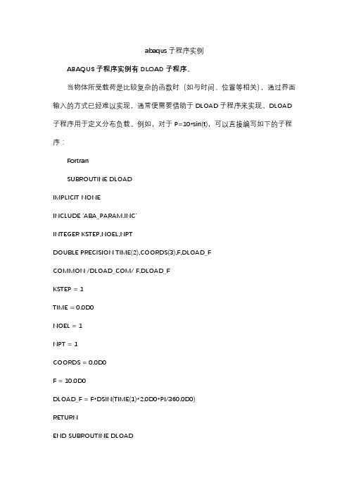
ABAQUS子程序实例有DLOAD子程序。

当物体所受载荷是比较复杂的函数时（如与时间、位置等相关），通过界面输入的方式已经难以实现，通常便需要借助于DLOAD子程序来实现。

DLOAD 子程序用于定义分布负载。

例如，对于P=10*sin(t)，可以直接编写如下的子程序：
Fortran
SUBROUTINE DLOAD
IMPLICIT NONE
INCLUDE 'ABA_PARAM.INC'
INTEGER KSTEP,NOEL,NPT
DOUBLE PRECISION TIME(2),COORDS(3),F,DLOAD_F
COMMON /DLOAD_COM/ F,DLOAD_F
KSTEP = 1
TIME = 0.0D0
NOEL = 1
NPT = 1
COORDS = 0.0D0
F = 10.0D0
DLOAD_F = F*DSIN(TIME(1)*2.0D0*PI/360.0D0)
RETURN
END SUBROUTINE DLOAD
上述程序中，已经明确指出user coding to define F，即表示需要用户自己去定义变量F的值，F的值便表示所加载的载荷大小。

该数值的正负符号有明确的物理意义，对于压力，正数表示压力，负数表示拉力。

也就是说只有F这个变量需要我们去定义，其它的一些变量都是输入变量，是软件传递给我们去使用的，不需要我们去定义。

《2024年ABAQUS用户材料子程序开发及应用》范文

《ABAQUS用户材料子程序开发及应用》篇一一、引言ABAQUS是一款功能强大的工程仿真软件，广泛应用于各种工程领域。

在ABAQUS中，用户材料子程序（User Material Subroutines）的开发与应用，对于提高仿真精度、模拟复杂材料行为具有重要意义。

本文将详细介绍ABAQUS用户材料子程序的开发过程，并探讨其在实际工程中的应用。

二、ABAQUS用户材料子程序开发1. 开发背景及意义ABAQUS提供了丰富的材料模型，但有时这些模型无法满足特定工程需求。

因此，用户可以通过编写自定义的材料子程序来模拟特定材料的行为。

用户材料子程序的开发，可以更好地反映材料的本构关系、力学性能等，从而提高仿真结果的准确性。

2. 开发流程（1）了解需求：明确仿真目标，了解所需模拟的材料特性。

（2）选择合适的子程序：根据需求，选择合适的用户材料子程序模板。

（3）编写代码：使用Fortran或C++等编程语言，编写描述材料行为的代码。

（4）编译及调试：将代码编译成可在ABAQUS中运行的动态链接库，并进行调试。

（5）在ABAQUS中集成：将编译好的动态链接库集成到ABAQUS中，进行仿真分析。

3. 开发注意事项（1）确保代码的准确性：编写代码时，应确保描述材料行为的数学模型正确，且代码实现无误。

（2）遵循ABAQUS编程规范：在编写代码时，应遵循ABAQUS的编程规范，以确保代码能够在ABAQUS中正常运行。

（3）进行充分的测试：在集成到ABAQUS之前，应对编写的代码进行充分的测试，确保其能够正确模拟材料行为。

三、ABAQUS用户材料子程序的应用1. 复杂材料模拟通过开发用户材料子程序，可以模拟复杂材料的本构关系、力学性能等。

例如，在金属成型、复合材料等领域，用户材料子程序可以帮助研究人员更好地了解材料在成型过程中的变形行为，为优化工艺提供依据。

2. 结构分析在结构分析中，用户材料子程序可以用于描述结构的力学性能、损伤演化等。

21ABAQUS用户材料子程序_1502407

21 ABAQUS用户材料子程序(UMAT)虽然ABAQUS为用户提供了大量的单元库和求解模型，使用户能够利用这些模型处理绝大多数的问题；但是实际问题毕竟非常复杂，ABAQUS不可能直接求解所有可能出现的问题。

所以ABAQUS提供了大量的用户自定义子程序（User Subroutine），允许用户在找不到合适模型的情况下自行定义符合自己问题的模型。

这些用户子程序涵盖了建模、载荷到单元的几乎各个部分。

用户子程序具有以下的功能和特点：（1）如果ABAQUS的一些固有选项模型功能有限，用户子程序可以提高ABAQUS中这些选项的功能；（2）通常用户子程序是用FORTRAN语言的代码写成；（3）它可以以几种不同的方式包含在模型中；（4）由于它们没有存储在restart文件中，如果需要的话，可以在重新开始运行时修改它；（5）在某些情况下它可以利用ABAQUS允许的已有程序。

要在模型中包含用户子程序，可以利用ABAQUS执行程序，在执行程序中应用user 选项指明包含这些子程序的FORTRAN源程序或者目标程序的名字。

提示：ABAQUS的输入文件除了可以通过ABAQUS/CAE的作业模块中提交运行外，还可以在ABAQUS Command窗口中输入ABAQUS执行程序直接运行：ABAQUS job=输入文件名 user=用户子程序的Fortran文件名ABAQUS/Standard和ABAQUS/Explicit都支持用户子程序功能，但是他们所支持的用户子程序种类不尽相同，读者在需要使用时请注意查询手册。

在接下来的两章里，我们将讨论两种常用的用户子程序——用户材料子程序和用户单元子程序。

本章将通过在ABAQUS/Standard中创建Johnson-Cook的材料模型，介绍编写ABAQUS/Standard的用户材料子程序UMAT。

在ABAQUS/Explicit中编写用户材料子程序VUMAT与之相似，但是由于隐式和显式两种方法本身的差异，它们之间也有一些不同，请读者在具体使用前仔细查阅ABAQUS手册中的相关内容。

1、下载文档前请自行甄别文档内容的完整性，平台不提供额外的编辑、内容补充、找答案等附加服务。
2、"仅部分预览"的文档,不可在线预览部分如存在完整性等问题,可反馈申请退款(可完整预览的文档不适用该条件!)。
3、如文档侵犯您的权益，请联系客服反馈,我们会尽快为您处理(人工客服工作时间：9:00-18:30)。

ABAQUS/Standard 用户材料子程序实例－Johnson-Cook 金属本构模型卢剑锋庄茁* 张帆清华大学工程力学系北京 100084摘要：用户材料子程序是ABAQUS 提供给用户定义自己的材料属性的Fortran 程序接口，使用户能使用ABAQUS 材料库中没有定义的材料模型。

ABAQUS 中自有的Johnson-Cook 模型只能应用于显式ABAQUS/Explicit 程序中，而我们希望能在隐式ABAQUS/Standard 程序中更精确的实现本构积分，而且应用Johnson-Cook 模型的修正形式。

这就需要通过ABAQUS/Standard 的用户材料子程序UMAT 编程实现。

在UMAT 编程中使用了率相关塑性理论以及完全隐式的应力更新算法。

1 Johnson-Cook 强化模型简介Johnson-Cook （JC ）模型用来模拟高应变率下的金属材料。

JC 强化模型表示为三项的乘积，分别反映了应变硬化，应变率硬化和温度软化。

这里使用JC 模型的修正形式：()()*01ln 11n m A B C T εσεε =+++−&& 并使参考应变率01ε=&，这样公式中的A 即为材料的静态屈服应力。

公式中包含,,,,A B n C m 五个参数，需要通过实验来确定。

2 ABAQUS 用户材料子程序用户材料子程序（User-defined Material Mechanical Behavior ，简称UMAT ）通过与ABAQUS 主求解程序的接口实现与ABAQUS 的数据交流。

在输入文件中，使用关键字“*USER MATERIAL”表示定义用户材料属性。

子程序概况与接口UMAT 子程序具有强大的功能，使用UMAT 子程序：(1) 可以定义材料的本构关系，使用ABAQUS 材料库中没有包含的材料进行计算，扩充程序功能。

(2)几乎可以用于力学行为分析的任何分析过程，几乎可以把用户材料属性赋予ABAQUS中的任何单元；(3)必须在UMAT中提供材料本构模型的雅可比（Jacobian）矩阵，即应力增量对应变增量的变化率。

(4)可以和用户子程序“USDFLD”联合使用，通过“USDFLD”重新定义单元每一物质点上传递到UMAT中场变量的数值。

由于主程序与UMAT之间存在数据传递，甚至共用一些变量，因此必须遵守有关UMAT的书写格式，UMAT中常用的变量在文件开头予以定义，通常格式为：SUBROUTINE UMAT(STRESS,STATEV,DDSDDE,SSE,SPD,SCD,1 RPL,DDSDDT,DRPLDE,DRPLDT,2 STRAN,DSTRAN,TIME,DTIME,TEMP,DTEMP,PREDEF,DPRED,CMNAME,3 NDI,NSHR,NTENS,NSTATV,PROPS,NPROPS,COORDS,DROT,PNEWDT,4 CELENT,DFGRD0,DFGRD1,NOEL,NPT,LAYER,KSPT,KSTEP,KINC)CINCLUDE 'ABA_PARAM.INC'CCHARACTER*80 CMNAMEDIMENSION STRESS(NTENS),STATEV(NSTATV),1 DDSDDE(NTENS,NTENS),DDSDDT(NTENS),DRPLDE(NTENS),2 STRAN(NTENS),DSTRAN(NTENS),TIME(2),PREDEF(1),DPRED(1),3 PROPS(NPROPS),COORDS(3),DROT(3,3),DFGRD0(3,3),DFGRD1(3,3)user coding to define DDSDDE, STRESS, STATEV, SSE, SPD, SCDand, if necessary, RPL, DDSDDT, DRPLDE, DRPLDT, PNEWDTRETURNENDUMAT中的应力矩阵、应变矩阵以及矩阵DDSDDE，DDSDDT，DRPLDE等，都是直接分量存储在前，剪切分量存储在后。

直接分量有NDI个，剪切分量有NSHR个。

各分量之间的顺序根据单元自由度的不同有一些差异，所以编写UMAT时要考虑到所使用单元的类别。

下面对UMAT中用到的一些变量进行说明：(),DDSDDE NTENS NTENS是一个NTENS维的方阵，称作雅可比矩阵，/σε，∆σ是应力的增量，∆ε是应变的增量，∂∆∂∆(),DDSDDE I J表示增量步结束时第J个应变分量的改变引起的第I个应力分量的变化。

通常雅可比是一个对称矩阵，除非在“*USER MATERIAL”语句中加入了“UNSYMM”参数。

()STRESS NTENS应力张量矩阵，对应NDI个直接分量和NSHR个剪切分量。

在增量步的开始，应力张量矩阵中的数值通过UMAT和主程序之间的接口传递到UMAT中，在增量步的结束UMAT将对应力张量矩阵更新。

对于包含刚体转动的有限应变问题，一个增量步调用UMAT之前就已经对应力张量的进行了刚体转动，因此在UMAT中只需处理应力张量的共旋部分。

UMAT中应力张量的度量为柯西（真实）应力。

()STATEV NSTATEV用于存储状态变量的矩阵，在增量步开始时将数值传递到UMAT中。

也可在子程序USDFLD 或UEXPAN中先更新数据，然后增量步开始时将更新后的数据传递到UMAT中。

在增量步的结束必须更新状态变量矩阵中的数据。

和应力张量矩阵不同的是：对于有限应变问题，除了材料本构行为引起的数据更新以外，状态变量矩阵中的任何矢量或者张量都必须通过旋转来考虑材料的刚体运动。

状态变量矩阵的维数，等于关键字“*DEPVAR”定义的数值。

状态变量矩阵的维数通过ABAQUS输入文件中的关键字“*DEPVAR”定义，关键字下面数据行的数值即为状态变量矩阵的维数。

材料常数的个数，等于关键字“*USER MATERIAL”中“CONSTANTS”常数设定的值。

()PROPS NPROPS材料常数矩阵，矩阵中元素的数值对应于关键字“*USER MATERIAL”下面的数据行。

SSE，SPD，SCD分别定义每一增量步的弹性应变能，塑性耗散和蠕变耗散。

它们对计算结果没有影响，仅仅作为能量输出。

其他变量：()STRAN NTENS：应变矩阵；()DSTRAN NTENS：应变增量矩阵；DTIME：增量步的时间增量；NDI：直接应力分量的个数；NSHR：剪切应力分量的个数；=+。

NTENS：总应力分量的个数，NTENS NDI NSHR使用UMAT时需要注意单元的沙漏控制刚度和横向剪切刚度。

通常减缩积分单元的沙漏控制刚度和板、壳、梁单元的横向剪切刚度是通过材料属性中的弹性性质定义的。

这些刚度基于材料初始剪切模量的值，通常在材料定义中通过“*ELASTIC”选项定义。

但是使用UMAT的时候，ABAQUS对程序输入文件进行预处理的时候得不到剪切模量的数值。

所以这时候用户必须使用“*HOURGLASS STIFFNESS”选项来定义具有沙漏模式的单元的沙漏控制刚度，使用“*TRANSVERSE SHEAR STIFFNESS”选项来定义板、壳、梁单元的横向剪切刚度。

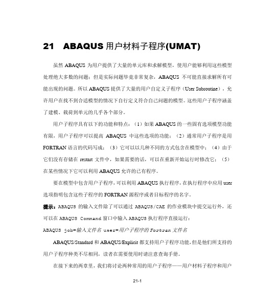
编程基于上面所述的率相关材料公式和应力更新算法，参照ABAQUS用户材料子程序的接口规范，进行UMAT的编程。

有限元模拟结果将在下一节给出，在最后一节中还给出了相应的程序源代码。

由于UMAT在单元的积分点上调用，增量步开始时，主程序路径将通过UMAT的接口进入UMAT，单元当前积分点必要变量的初始值将随之传递给UMAT的相应变量。

在UMAT结束时，变量的更新值将通过接口返回主程序。

整个UMAT的流程如图1所示。

一共有8个材料常数需要给定，并申请一个13维的状态变量矩阵，它们表示的物理含义如表1所示。

下一步将使用建立的UMAT结合ABAQUS/Standard进行霍布金森冲击杆(SHPB)实验的有限元模拟，并对结果进行比较。

图1 UMAT流程图表1 UMAT材料常数PROPS 1 2 3 4 5 6 7 8物理性质杨氏模量泊松比塑性耗散比 A B n C MSTATEV 1-6 7-12 13变量意义弹性应变塑性应变等效塑性应变3 SHPB实验的有限元模拟模型的简化与有限元网格为了不使模型过于庞大，对模型进行了一些简化。

首先，改变入力杆和出力杆的尺寸，长度由原来的3040mm减小为1000mm，直径增加到25mm，试件的长度和直径也分别变化为22mm 和18mm。

这样不仅优化了网格的质量，还成倍地减小了模型的规模，其带来的负面影响就是试件能达到的应变将降低。

另外，由于撞击杆仅仅起到产生应力脉冲的作用，在数值模型中没必要考虑撞击杆，取代的方法是直接在入力杆的输入端施加均布的应力脉冲。

考虑到实验装置的对称性，也做了一些简化。

整个实验装置以及载荷等都是关于杆的中心线轴对称的，所以可以使用轴对称单元进行二维分析。

二维轴对称模型如图2所示。

在模型中，对试件以及入力杆，出力杆和试件接触的部分进行了局部网格加密，这样的网格划分可以取得比较经济的结果。

图2 二维轴对称有限元模型表2 模型信息模型尺寸[mm] (Φ×L ) 单元类型单元个数总节点数总单元数入力杆 25×1000 CAX4 530 试件 18×22 CAX4 160 二维模型出力杆 25×1000 CAX4 530 1475 1220 材料定义入力杆和出力杆使用线弹性材料，弹性模量和泊松比分别为200GPa 和0.3，密度为7.85×103 kg/m 3。

试件采用用户在UMAT 中自定义材料，材料参数如表3所示，其中Johnson-Cook 模型中参数的数值来源于前面的数值拟合程序。

表3 试件的材料定义 Johnson-Cook 模型参数性质密度 [Kg/m 3] 杨氏模量 [MPa] 泊松比 A [MPa ] B [MPa] n C M 数值 2.7×103 68.0×103 0.33 66.562 108.8530.238 0.029 0.5。