石油工程 CH13
石油工程项目管理机制

关, 与承 包 商 的边 际生 产 率 正 相 关 , 与 其他 可观 测 变 量 相 关 。在 最 优 监 督 水 平 下 , 业 公 司 的 边 际 生 产 率 越 高 , 际 成 还 作 边 本 越 低 , 容 易监 督 , 督 带 来 的边 际 收 益越 高 。 对于 那 些 监督 比较 困难 的项 目, 以通 过 加 强 惩 罚 力 度 的 方 式 弥 补 难 以 越 监 可 有 效 监 督 的 不足 。 激 励 性 承包 方 式 可 以减 小 逆 向选 择 造 成 的危 害 , 建 动 态联 盟 可 以 进 一 步加 强 激 励 作 用 , 组 降低 道 德 风
r s rc e viec m p is e fc i l l s h y s er ie t e c e t its r c o ane fe tvey un e st e up vs h onta t f r c of wor . I h i a onta t s k n t eoptm lc r c s,i en i ei de s nc tv n x i
维普资讯
石
22 4 20 0 6年 4月 油勘探与开发
Vo . 3 No 2 13 .
PE TROL EUM EXPL ORATI ON AND DEVEL OPM ENT
文 章 编 号 :0 0 0 4 ( 0 6 0 — 2 20 1 0 — 7 7 2 0 ) 20 4 —4
石 油 工程 项 目管 理 机 制
罗 东坤 , 治 国 丁
( 国 石油 大 学 ( 京) 中 北 ) 基 金 项 目 : 家 高技 术 研 究发 展 计 划 “ 6 ” 目“ 国 83项 可控 ( 闭环 ) 维轨 迹 钻 井技 术 ” 2 0 AA6 2 1 - 3 三 (01 0 0 20 B)
石油工程类SCI期刊

2013年SCIE收录石油期刊24种,其中SCI收录9种。
2012年JCR收录石油期刊24种,其中影响因子1以上有4种、影响因子0.5以上有7种,2012年石油期刊影响因子前5名期刊如下:1、 AAPG BULLETIN《美国石油地质学家协会通报》Monthly ISSN: 0149-1423,2012年影响因1.768、5年影响因子2.4552、PETROLEUM GEOSCIENCE《石油地质科学》 Quarterly ISSN: 1354-0793,2012年影响因1.500、5年影响因子1.2503、OIL & GAS SCIENCE AND TECHNOLOGY-REVUE D IFP ENERGIES NOUVELLES《石油、天然气的科学与技术;法国石油研究所杂志》Bimonthly ISSN: 1294-4475,2012年影响因1.258、5年影响因子1.3674、SPE JOURNAL《石油工程师协会杂志》 Quarterly ISSN: 1086-055X,2012年影响因1.011、5年影响因子1.4635、JOURNAL OF PETROLEUM SCIENCE AND ENGINEERING《石油科学和石油工程杂志》 Monthly ISSN: 0920-4105,2012年影响因0.997、5年影响因子1.2972013年SCI收录石油学科期刊24种目录SCIENCE CITATION INDEX EXPANDEDENGINEERING, PETROLEUM - JOURNAL LIST Total journals: 241. AAPG BULLETIN《美国石油地质学家协会通报》Monthly ISSN: 0149-1423AMER ASSOC PETROLEUM GEOLOGIST, 1444 S BOULDER AVE, PO BOX 979, TULSA, USA, OK, 74119-36042. CHEMISTRY AND TECHNOLOGY OF FUELS AND OILS《燃料与石油化学和工艺学》Bimonthly ISSN: 0009-3092SPRINGER, 233 SPRING ST, NEW YORK, USA, NY, 100133. CHINA PETROLEUM PROCESSING & PETROCHEMICAL TECHNOLOGY《中国炼油与石油化工》 Quarterly ISSN: 1008-6234CHINA PETROLEUM PROCESSING & PETROCHEMICAL TECHNOLOGY PRESS, NO 18 XUEYUAN RD, BEIJING, PEOPLES R CHINA, 1000834. CT&F-CIENCIA TECNOLOGIA Y FUTURO Annual ISSN: 0122-5383ECOPETROL SA, INST COLOMBIANO PETROLEO, CONSEJO EDITORIAL CT F,KILOMETRO 7 VIA BUCARAMANGA, BOGOTA, COLOMBIA, 000005. HYDROCARBON PROCESSING《烃加工》Monthly ISSN: 0018-8190GULF PUBL CO, BOX 2608, HOUSTON, USA, TX, 77252-26086. INTERNATIONAL JOURNAL OF OIL GAS AND COAL TECHNOLOGY《国际石油、天然气与煤炭技术杂志》 Quarterly ISSN: 1753-3309INDERSCIENCE ENTERPRISES LTD, WORLD TRADE CENTER BLDG, 29 ROUTE DE PRE-BOIS, CASE POSTALE 856, GENEVA, SWITZERLAND, CH-12157. JOURNAL OF CANADIAN PETROLEUM TECHNOLOGY《加拿大石油技术杂志》 Monthly ISSN: 0021-9487SPE-SOC PETROLEUM ENGINEERS, CANADA, 500-5 AVE SW, STE 425, CALGARY, CANADA, ALBERTA, T2P 3L58. JOURNAL OF GEOPHYSICS AND ENGINEERING《地球物理学与工程学》 Irregular ISSN: 1742-2132IOP PUBLISHING LTD, TEMPLE CIRCUS, TEMPLE WAY, BRISTOL, ENGLAND, BS1 6BE9. JOURNAL OF PETROLEUM GEOLOGY《石油地质学杂志》 Quarterly ISSN: 0141-6421WILEY-BLACKWELL, 111 RIVER ST, HOBOKEN, USA, NJ, 07030-577410. JOURNAL OF PETROLEUM SCIENCE AND ENGINEERING《石油科学和石油工程杂志》Monthly ISSN: 0920-4105ELSEVIER SCIENCE BV, PO BOX 211, AMSTERDAM, NETHERLANDS, 1000 AE11. JOURNAL OF THE JAPAN PETROLEUM INSTITUTE《日本石油学会志》 Bimonthly ISSN: 1346-8804JAPAN PETROLEUM INST, COSMO HIRAKAWA-CHO BLDG, 3-14, 1-CHOMEHIRAKAWA-CHO, CHIYODA-KU, TOKYO, JAPAN, 10212. OIL & GAS JOURNAL《石油与天然气杂志》 Weekly ISSN: 0030-1388PENNWELL PUBL CO ENERGY GROUP, 1421 S SHERIDAN RD PO BOX 1260, TULSA, USA, OK, 7411213. OIL & GAS SCIENCE AND TECHNOLOGY-REVUE D IFP ENERGIES NOUVELLES《石油、天然气的科学与技术;法国石油研究所杂志》Bimonthly ISSN: 1294-4475EDITIONS TECHNIP, 27 RUE GINOUX, PARIS 15, FRANCE, 7573714. OIL GAS-EUROPEAN MAGAZINE《欧洲石油气杂志》 Quarterly ISSN: 0342-5622URBAN-VERLAG GMBH, PO BOX 70 16 06, HAMBURG, GERMANY, D-2201615. OIL SHALE《油页岩》Quarterly ISSN: 0208-189XESTONIAN ACADEMY PUBLISHERS, 6 KOHTU, TALLINN, ESTONIA, 1013016. PETROLEUM CHEMISTRY《石油化学》 Bimonthly ISSN: 0965-5441MAIK NAUKA/INTERPERIODICA/SPRINGER, 233 SPRING ST, NEW YORK, USA, NY, 10013-157817. PETROLEUM GEOSCIENCE《石油地质科学》 Quarterly ISSN: 1354-0793GEOLOGICAL SOC PUBL HOUSE, UNIT 7, BRASSMILL ENTERPRISE CENTRE,BRASSMILL LANE, BATH, ENGLAND, AVON, BA1 3JN18. PETROLEUM SCIENCE《石油科学》Quarterly ISSN: 1672-5107SPRINGER HEIDELBERG, TIERGARTENSTRASSE 17, HEIDELBERG, GERMANY,D-6912119. PETROLEUM SCIENCE AND TECHNOLOGY《石油科学与技术》Semimonthly ISSN: 1091-6466TAYLOR & FRANCIS INC, 325 CHESTNUT ST, SUITE 800, PHILADELPHIA, USA, PA, 1910620. PETROPHYSICS《岩石物理学》 Bimonthly ISSN: 1529-9074SOC PETROPHYSICISTS & WELL LOG ANALYSTS-SPWLA, 8866 GULF FREEWAY, STE 320, HOUSTON, USA, TX, 7701721. SPE DRILLING & COMPLETION《石油工程师协会钻井与完井》 Quarterly ISSN: 1064-6671SOC PETROLEUM ENG, 222 PALISADES CREEK DR,, RICHARDSON, USA, TX, 7508022. SPE JOURNAL《石油工程师协会杂志》 Quarterly ISSN: 1086-055XSOC PETROLEUM ENG, 222 PALISADES CREEK DR,, RICHARDSON, USA, TX, 7508023. SPE PRODUCTION & OPERATIONS《石油工程师协会生产和操作》 Quarterly ISSN: 1930-1855SOC PETROLEUM ENG, 222 PALISADES CREEK DR,, RICHARDSON, USA, TX, 7508024. SPE RESERVOIR EVALUATION & ENGINEERING《石油工程师协会油藏评估与工程》Bimonthly ISSN: 1094-6470SOC PETROLEUM ENG, 222 PALISADES CREEK DR,, RICHARDSON, USA, TX, 75080。
化学名词(石油化学)

1、石脑油:简称NAP ,又称粗汽油,是石油轻质馏分的泛称。
由原油蒸馏或石油二次加工而得。
主要成分为烷烃的C 4~C 6。
主要用途:可分离出汽油、苯、煤油、沥青等多种有机原料。
是裂解制取乙烯、丙烯,催化重整制取苯,甲苯,二甲苯的重要原料。
2、苯:分子式C 6H 6,结构式。
苯是最简单的芳香烃。
苯是一种石油化工基本原料。
苯的产量和生产的技术水平是一个国家石油化工发展水平的标志之一。
3、甲苯:分子式C 7H 8,结构式,是一种无色,带特殊芳香味的易挥发液体,简称MB 。
甲苯是芳香烃的一种,是一种常用的化工原料,可用于制造炸药、农药、苯甲酸、染料、合成树脂及涤纶等。
同时它也是汽油的一个组成成分。
4、二甲苯:又称1,2-二甲苯,分子式C 6H 4(CH 3)2,简称DMB 。
为无色透明液体,有邻、间、对三种异构体。
由芳烃联合装置的重整液、加氢汽油分馏以及甲苯歧化得到混合二甲苯。
在工业上,二甲苯即指上述异构体的混合物。
广泛用于涂料、树脂、染料、油墨等行业做溶剂;用于医药、炸药、农药等行业做合成单体或溶剂;也可作为高辛烷值汽油组分,是有机化工的重要原料。
5、对二甲苯:又称1,4-二甲苯,分子式C 8H 10,结构式,是苯的衍生物,重要的化工原料,简称PX 。
混合二甲苯经吸附分离制取可得到对二甲苯。
主要用于制造对苯二甲酸,可用于化工及制药工业等。
也是用于生产聚对苯二甲酸乙二醇酯(PET)的重要中间体。
PET 纤维又称聚酯纤维或涤纶纤维,是一种常用的化学合成纤维。
—CH 3—CH 3CH 3—6、乙烯:乙烯是由两个碳原子和四个氢原子组成的化合物,分子式为C 2H 4,结构式。
乙烯是合成纤维、合成橡胶、合成塑料、合成乙醇的基本化工原料,也用于制造氯乙烯、苯乙烯、环氧乙烷、醋酸、乙醛、乙醇和炸药等。
7、聚乙烯:是乙烯经聚合制得的一种热塑性树脂简称,结构式,简称PE 。
聚乙烯为白色蜡状半透明材料,柔而韧,比水轻,无毒,具有优越的介电性能。
石油溶剂知识

馏程:纯化合物都有一定的沸点,但石油及其产品则是一个主要由多种烃类及少量烃类衍生物组成的复杂混合物,其沸点表现为一很宽的范围,是沸点连续的多组分的混合物,因而石油产品没用一个确定的沸点,通常以该产品的沸点范围或馏程表示。
当加热石油产品时,首先蒸发出来的主要是分子量小的,沸点低的组分,随着加热温度的升高,分子量大的,沸点高的也逐渐蒸发出来,直到最后高沸点的物质全部蒸发出来为止。
油品在规定条件下,蒸馏所得到的以初馏点和终馏点表示其蒸发特征的温度范围叫馏程。
馏程规定的实质是将一定体积或重量的油品加热蒸馏,测出各溜出量的相应温度,或相当于一定馏出温度的馏出量。
初馏点:在恩氏蒸馏设备里,当油品加热蒸馏出来第一滴油品时,记录下来的油蒸汽温度。
终馏点:当油品基本上全部蒸馏出来时,油蒸汽温度达最高温度叫油品的干点又叫终馏点。
闪点:又叫闪燃点,是指可燃性液体表面上的蒸汽和空气的混合物与火接触而初次发生闪光时的温度。
各种油品的闪点可通过标准仪器测定。
闪点温度比着火点温度低些。
液体闪点就是可能引起火灾的最低温度。
闪点越低,引起火灾的危险性越大。
燃点:又叫着火点,是指可燃性液体表面上的蒸汽和空气的混合物与火接触而发生火焰能继续燃烧不少于5s时的温度。
可在测定闪点后继续在同一标准仪器中测定。
可燃性液体的闪点和燃点表明其发生爆炸或火灾的可能性的大小,对运输、储存和使用的安全有极大关系。
倾点:是指油品在规定的试验条件下,被冷却的试样能够流动的最低温度。
凝点:是指油品在规定的试验条件下,被冷却的试样油面不再移动时的最高温度,都以℃表示。
是用来衡量润滑油低温流动性的常规指标,同一油品的倾点比凝点略高几度,过去常用凝点,现在国际通用倾点。
倾点或凝点偏高,油品的低温流动性就差。
人们可以根据油品倾点的高低,考虑在低温条件下运输、储存、收发时应该采取的措施,也可以用来评估某些油口的低温使用性能。
苯胺点:在标准试验条件下石油产品与等体积的苯胺,在互相溶解成为单一液相的最低温度叫苯胺点。
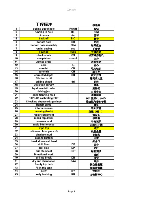
缩写_英语石油工程标注和部分缩写
Page 2
工程标注
93 94 95 96 97 98 99 100 101 102 103 104 117 118 119 120 121 122 123 124 125 126 127 128 129 130 131 132 133 134 135 136 137 138 139 140 141 142 143 144 145 146 147 148 149 150 151
kick lost circulation water flowing lost mud loss losses over haul repair pump lay on blow out preventer swivvel cut off work line slip work line stop check chain block killing well kill the well close well head hole junk basket fish fishing job fish up back off overshot well loggint casing program casing shoe ahead water rear water cementing cemented up wait on cement finish cement plug fill up wait on matterial standby production test setting slip bushing elevator elevator tink rotary table rat hole
Page 3
工程标注
152 153 154 155 156 157 158 159 160 161 162 163 164 165 166 167 168 169 170 171 172 173 174 175 176 177 178 179 180 181 182 183 184 185 186 187 188 189 190 191 192 193 194 195 196 197 198
采油工程(井基本流动规律)

(1-4)
(1) 采油指数
例: A井 100吨/天 B井 80吨/天
A井 110吨/天
如果 若
B井 120吨/天
Pwf ,则P, qA ,qB qB qA ,则B井产能大。
q P
衡量产能: 采油指数
采油指数:油井日产量与生产压差的比值。
它表示单位生产压差下油井的日产量, 用以衡量油井的生产能力。
Ko Kw qL Ch JL Pe Pwf ln re rw S Bo o Bw w
采油指数反映了地层参数,反过来说, 地层参数影响采油指数。
(3) 流入动态关系曲线
①流入动态关系
根据(1-2a)式:qo =Jo(Pe-Pwf) 一般,在一定时期内: J=C(单相渗流), Pe=C
Pe C
Pw
( 1-1a )
参见: DAKE : Fundamentals of Reservoir Engineering
(3)
非圆边界的产量公式
A—泄流面积;
Cx值见P3 图1—2
2、 采油指数及流入动态
q0 h ( Pe Pwf ) re o B o (ln S) rw CK
Pwf q0 / 1 0.2 Pwf / Pr 0.8 Pr
2
解:(1) 求:q0max
qo max
2 11 11 0.8 30 / 1 0.2 13 13 3 116.3m / d
reh 区域的长半轴; a L 0.5 0.25 2 L/2
4
(1-9)
L——水平井水平段长度(简称井长); S——水平井表皮系数; reh——水平井的泄流半径
油气储运工程相关期刊

油气储运专业相关期刊看文献, 发论文?期刊水平如何?现将油气储运专业论文常见的期刊整理如下,低共分5类:SCI 核心,SCIE El,―※SCI 核心1. 《科学》Scienee (周刊,美国,2. 《自然》Nature (周刊,英国,3. 《石油工程师协会杂志》4. 《石油科学和石油工程杂志》ISSN: 0920-4105, SCI ) 5《. 石油、天然气的科学与技术 -法国石油研究所杂志》 (双月刊, 法国, ISSN:1294-4475, SCI )Oil & Gas Science And Technology-Revue D IFP Energies Nouvelles 6. 《中国科学-化学•英文版》(月刊,中科院主办,ISSN 1674-7291 , SC ) 7.《化学学报•中文版》 Acta Chimica Sinica (半月刊,中科院主办, ISSN 0567-7351 , SC )8. 《物理学报-中文版》Acta Physica Sinica (半月刊,中国物理学会主办,ISSN 1000-3290 ,SCI ) 9.《高等学校化学学报•中文版》 Chemical Journal of Ch ineseU Diversities (月刊,吉林大学主办, ISSN :0251-0790, SCI )10. 《中国化学-英文版》Chinese Journalof Chemistry (月刊,中国化学会主办,ISSN 1001-604X,SCI )11. 《中国物理快报-英文版》Chinese Physics Lette (月刊,中国物理学会主办,ISSM 0256-307X, SCI )12. 《国际多相流杂志》 (月刊,英国, ISSN : 0301-9322, SC )I INTERNATIONAL JOURNAL OF MULTIPHASEFLOW13. 《化学工程研究与设计》 (月刊,英国, ISSN : 0263-8762, SCI ) CHEMICAL ENGINEERING RESEARCH &DESIGN14. 《化工科学》 (半月刊,英国, ISSN : 0009-2509, SCI ) CHEMICAL ENGINEERING SCIENCE15. 《粉末技术》 (半月刊,瑞士, ISSN : 0032-5910, SCI ) POWDER TECHNOLOGY16. 《流变学杂志》 (双月刊,美国, ISSN : 0148-6055, SC )I JOURNAL OF RHEOLOGY17. 《非牛顿流体力学杂志》 (半月刊,荷兰, ISSN : 0377-0257, SCI )Journal of Non-Newtonian FluidMechanics18. 《胶体与界面科学杂志》 (半月刊,美国, ISSN : 0021-9797, SCI ) JOURNAL OF COLLOID AND INTERFACESCIENCE19. 《兰茂尔》LANGMUIR (周刊,美国,ISSN 0743-7463, SC )水平从高到 中文核心, 非核心杂志 (各类均包含的以最高类别为准) 。
石油加工热加工过程

2020/6/24
石油加工工程
28
1. 8. 最近国内新建装置常采用对流串辐射工艺,原料油经换热后先进原 料缓冲罐,然后泵送进加热炉对流段与辐射段连续加热,不再由对流 段后抽出进分馏塔换热,这样可以灵活调控循环比。
2. 9. 由于延迟焦化的操作是循环式操作,带来许多操作连锁影响问题, 例如压力变动、温度变动、操作不稳等,又如焦炭塔塔顶油气携带焦 粉会促使大油气管线和分馏塔塔底结焦,加热炉进料中含有焦粉会促 进炉管结焦,在炭化过程中这些焦粉促进缩合使焦炭产率增大,使焦 炭的机械强度降低,容易产生粉焦等。
3.渣油在热过程中可发生相分离
渣油是一种胶体分散体系
2020/6/24
石油加工工程
14
2020/6/24
石油加工工程
15
渣油热反应产物分布随时间的变化 1-原料; 2-中间馏分; 3-汽油; 4-裂化气; 5-残油; 6-焦炭
2020/6/24
石油加工工程
16
裂化 产物
裂
化断 侧 链
饱和烃 脱
应速率常数与反应温度的关系服从阿累尼乌斯方程;
➢ 在实际计算中,使用反应速率常数的温度系数 kt 有时更
为方便。Kt 的定义是:
➢ 对于烃类热裂解反应而言, Kt 值约在1.5 - 2.0之间,即
反应温度每升高10℃则反应速率约提高到原反应速率的 1.5 - 2.0倍。
2020/6/24
石油加工工程
2020/6/24
石油加工工程
27
4. 对加热炉最重要的要求是炉膛的热分布良好、各部分炉管 的表面热强度均匀、而且炉管环向热分布良好,避免局部 过热的现象发生
5. 延迟焦化装置常用的炉型是双面加热无焰燃烧炉 6. 延迟焦化装置采用水力除焦,利用高压水(约120巴)从水
- 1、下载文档前请自行甄别文档内容的完整性,平台不提供额外的编辑、内容补充、找答案等附加服务。
- 2、"仅部分预览"的文档,不可在线预览部分如存在完整性等问题,可反馈申请退款(可完整预览的文档不适用该条件!)。
- 3、如文档侵犯您的权益,请联系客服反馈,我们会尽快为您处理(人工客服工作时间:9:00-18:30)。
Reservoirs containing only free gas are termed gas reservoirs. Such a reservoir contains a mixture of hydrocarbons, which exists wholly in the gaseous state. The mixture may be a dry, wet,or condensate gas, depend-ing on the composition of the gas, along with the pressure and tempera-ture at which the accumulation exists.Gas reservoirs may have water influx from a contiguous water-bearing portion of the formation or may be volumetric (i.e., have no water influx).Most gas engineering calculations involve the use of gas formation volume factor B g and gas expansion factor E g. Both factors are defined in Chapter 2 by Equations 2-52 through 2-56. Those equations are summa-rized below for convenience:• Gas formation volume factor B g is defined is defined as the actual vol-ume occupied by n moles of gas at a specified pressure and tempera-ture, divided by the volume occupied by the same amount of gas at standard conditions. Applying the real gas equation-of-state to both conditions gives:• The gas expansion factor is simply the reciprocal of B g, or:ETppzTpzTgscsc==3537.(13-2)BpTzTpzTpgscsc==002827.(13-1)827C H A P T E R13GAS RESERVOIRSwhere B g=gas formation volume factor, ft3/scfE g=gas expansion factor, scf/ft3This chapter presents two approaches for estimating initial gas in place G, gas reserves, and the gas recovery for volumetric and water-drive mechanisms:• V olumetric method• Material balance approachTHE VOLUMETRIC METHODData used to estimate the gas-bearing reservoir PV include, but are not limited to, well logs, core analyses, bottom-hole pressure (BH P) and fluid sample information, along with well tests. This data typically is used to develop various subsurface maps. Of these maps, structural and stratigraphic cross-sectional maps help to establish the reservoir’s areal extent and to identify reservoir discontinuities, such as pinch-outs, faults, or gas-water contacts. Subsurface contour maps, usually drawn relative to a known or marker formation, are constructed with lines connecting points of equal elevation and therefore portray the geologic structure. Subsurface isopachous maps are constructed with lines of equal net gas-bearing formation thickness. With these maps, the reservoir PV can then be estimated by planimetering the areas between the isopachous lines and using an approximate volume calculation technique, such as the pyrami-dal or trapezoidal method.The volumetric equation is useful in reserve work for estimating gas in place at any stage of depletion. During the development period before reservoir limits have been accurately defined, it is convenient to calculate gas in place per acre-foot of bulk reservoir rock. Multiplication of this unit figure by the best available estimate of bulk reservoir volume then gives gas in place for the lease, tract, or reservoir under consideration. Later in the life of the reservoir, when the reservoir volume is defined and performance data are available, volumetric calculations provide valuable checks on gas in place estimates obtained from material balance methods. The equation for calculating gas in place is:GAh SBwigi=-435601,()f(13-3)828Reservoir Engineering Handbookwhere G =gas in place, scfA =area of reservoir, acresh =average reservoir thickness, ftf =porosityS wi =water saturation, andB gi =gas formation volume factor, ft 3/scfThis equation can be applied at both initial and abandonment condi-tions in order to calculate the recoverable gas.Gas produced =Initial gas -Remaining gasorwhere B ga is evaluated at abandonment pressure. Application of the volu-metric method assumes that the pore volume occupied by gas is constant.If water influx is occurring, A, h, and S w will change.Example 13-1A gas reservoir has the following characteristics:A =3000 acresh =30 ft f =0.15S wi =20%T =150°F p i =2600 psip z26000.8210000.884000.92Calculate cumulative gas production and recovery factor at 1000 and 400 psi.G Ah S B B p wi gi ga =--ÊËÁˆ¯˜43560111,()f (13-4)Gas Reservoirs 829SolutionStep 1.Calculate the reservoir pore volume P.VP.V=43,560 Ah fP.V=43,560 (3000) (30) (0.15) =588.06 MMft3Step 2.Calculate B g at every given pressure by using Equation 13-1.p z B g, ft3/scf26000.820.005410000.880.01524000.920.0397Step 3.Calculate initial gas in place at 2600 psiG=588.06 (106) (1 -0.2)/0.0054=87.12 MMMscfStep 4.Since the reservoir is assumed volumetric, calculate the remain-ing gas at 1000 and 400 psi.• Remaining gas at 1000 psiG1000 psi=588.06(106) (1 -0.2)/0.0152=30.95 MMMscf• Remaining gas at 400 psiG400 psi=588.06(106) (1 -0.2)/0.0397=11.95 MMMscfStep 5.Calculate cumulative gas production G p and the recovery factor RF at 1000 and 400 psi.• At 1000 psi:G p=(87.12-30.95)¥109=56.17 MMM scfRF=¥¥= 5617108712106459...%830Reservoir Engineering Handbook• At 400 psi:G p =(87.12-11.95) ¥109=75.17 MMMscfThe recovery factors for volumetric gas reservoirs will range from 80to 90%. If a strong water drive is present, trapping of residual gas at higher pressures can reduce the recovery factor substantially, to the range of 50 to 80%.THE MATERIAL BALANCE METHODIf enough production-pressure history is available for a gas reservoir,the initial gas in place G, the initial reservoir pressure p i , and the gas reserves can be calculated without knowing A, h, f , or S w . This is accom-plished by forming a mass or mole balance on the gas as:n p =n i -n f(13-5)where n p =moles of gas producedn i =moles of gas initially in the reservoirn f =moles of gas remaining in the reservoirRepresenting the gas reservoir by an idealized gas container, as shown schematically in Figure 13-1, the gas moles in Equation 13-5 can be replaced by their equivalents using the real gas law to give:where p i =initial reservoir pressureG p =cumulative gas production, scfp =current reservoir pressureV =original gas volume, ft 3z i =gas deviation factor at p i z =gas deviation factor at pT =temperature, °RW e =cumulative water influx, ft 3W p =cumulative water production, ft 3p G R T p V z RT p V W W zRT sc psc i i e p =---[()](13-6)RF =¥¥=75171087121086399...%Gas Reservoirs 831Equation 13-6 is essentially the general material balance equation (MBE). Equation 13-6 can be expressed in numerous forms depending on the type of the application and the driving mechanism. In general, dry gas reservoirs can be classified into two categories:• V olumetric gas reservoirs• Water-drive gas reservoirsThe remainder of this chapter is intended to provide the basic back-ground in natural gas engineering. There are several excellent textbooks that comprehensively address this subject, including the following:• Ikoku, C., Natural Gas Reservoir Engineering,1984• Lee, J. and Wattenbarger, R., Gas Reservoir Engineering,SPE, 1996Volumetric Gas ReservoirsFor a volumetric reservoir and assuming no water production, Equa-tion 13-6 is reduced to:p G T p z T V p zT V sc pi =ÊËÁˆ¯˜-Êˈ¯(13-7)Figure 13-1.Idealized water-drive gas reservoir.Figure 13-2.Gas material balance equation.The original gas volume V can be calculated from the slope and used to determine the areal extend of the reservoir from:V =43,560 Ah f (1-S wi )(13-10)where A is the reservoir area in acres.• Intercept at G p =0 gives p i /z i • Intercept at p/z =0 gives the gas initially in place G in scf• Cumulative gas production or gas recovery at any pressure Example 13-21A volumetric gas reservoir has the following production history.Time, tReservoir pressure, p Cumulative production, G pyears psia zMMMscf 0.017980.8690.000.516800.8700.961.015400.880 2.121.514280.890 3.212.013350.900 3.92The following data is also available:f =13%S wi =0.52A =1060 acresh =54 ft.T =164°FCalculate the gas initially in place volumetrically and from the MBE.SolutionStep 1.Calculate B gi from Equation 13-1B ft scf gi =+=002827086916446017980008533.(.)()./834Reservoir Engineering Handbook1After Ikoku, C., Natural Gas Reservoir Engineering,John Wiley & Sons, 1984.Figure 13-3.Relationship of p/z vs. G p for Example 13-2.Figure 13-4.Effect of water drive on p/z vs. G p relationship.Figure 13-5.An energy plot.l o g 1–z i p p i z ÊËÁˆ¯˜since the increasing slope would imply that the gas-occupied pore vol-ume was increasing with time.Form 2. In terms of B gFrom the definition of the gas formation volume factor, it can be expressed as:Combining the above expression with Equation 13-1 gives:where V =volume of gas originally in place, ft 3G =volume of gas originally in place, scf p i =original reservoir pressure z i =gas compressibility factor at p iEquation 13-13 can be combined with Equation 13-7, to give:Equation 13-14 suggests that to calculate the initial gas volume, the only information required is production data, pressure data, gas specific gravity for obtaining z-factors, and reservoir temperature. Early in the producing life of a reservoir, however, the denominator of the right-hand side of the material balance equation is very small, while the numerator is relatively large. A small change in the denominator will result in a large discrepancy in the calculated value of initial gas in place. There-fore, the material balance equation should not be relied on early in the producing life of the reservoir.Material balances on volumetric gas reservoirs are simple. Initial gas in place may be computed from Equation 13-14 by substituting cumula-tive gas produced and appropriate gas formation volume factors at corre-sponding reservoir pressures during the history period. If successive cal-culations at various times during the history give consistent values for initial gas in place, the reservoir is operating under volumetric controlG G B B B p g g gi=-(13-14)p T z T p VGsc sc i i =(13-13)B V Ggi =Figure 13-6.Graphical determination of the gas initially in place G.b. Recalculate the gas initially in place assuming that the pressure mea-surements were incorrect and the true average pressure is 2900 psi.The gas formation volume factor at this pressure is 0.00558 ft 3/scf.Solutiona. Using Equation 13-14, calculate G.b. Recalculate G by using the correct value of B g .Thus, an error of 100 psia, which is only 3.5% of the total reservoir pressure, resulted in an increase in calculated gas in place of approxi-mately 160%, a 21⁄2-fold increase. Note that a similar error in reservoir pressure later in the producing life of the reservoir will not result in an error as large as that calculated early in the producing life of the reservoir.Water-Drive Gas ReservoirsIf the gas reservoir has a water drive, then there will be two unknowns in the material balance equation, even though production data, pressure,temperature, and gas gravity are known. These two unknowns are initial gas in place and cumulative water influx. In order to use the material bal-ance equation to calculate initial gas in place, some independent method of estimating W e , the cumulative water influx, must be developed as dis-cussed in Chapter 11.Equation 13-14 can be modified to include the cumulative water influx and water production to give:The above equation can be arranged and expressed as:G W B B G B W B B B eg gi p g p w g gi+-=+-(13-16)G G B W W B B B p g e p w g gi=---()(13-15)G MMMscf=¥-=36010000668000558000527866526(.)...G MMMscf =¥-=360100005390005390005278173256(.)...Figure 13-7.Effect of water influx on calculating the gas initially in place.MATERIAL BALANCE EQUATIONAS A STRAIGHT LINEHavlena and Odeh (1963) expressed the material balance in terms of gas production, fluid expansion, and water influx as:Underground Gas Water expansion/Water =++withdrawal expansionpore compactioninfluxorUsing the nomenclature of Havlena and Odeh, as described in Chapter 11, gives:F =G (E g +E f,w )+W e B w(13-18)with the terms F, E g , and E f,w as defined by:• Underground fluid withdrawal F:F =G p B g +W p B w (13-19)• Gas expansion E g :E g =B g -B gi(13-20)• Water and rock expansion E f,w :Assuming that the rock and water expansion term E f,w is negligible in comparison with the gas expansion E g , Equation 13-18 is reduced to:F =G E g +W e B w(13-22)E B c S c S f w giw wi f wi,()=+-1(13-21)G B W B G B B G B c S c S pW B p g p w g gi giw wi f wie w+=-++-+()()1D (13-17)Figure 13-8.Defining the reservoir-driving mechanism.Figure 13-9.Havlena-Odeh MBE plot for a gas reservoir.say, at six monthly intervals, should plot as a straight line parallel to the abscissa—whose ordinate value is the GIIP.Alternatively, if the reservoir is affected by natural water influx then the plot of F/E g will usually produce a concave downward shaped arc whose exact form is dependent upon the aquifer size and strength and the gas off-take rate. Backward extrapolation of the F/E g trend to the ordi-nate should nevertheless provide an estimate of the GIIP(W e~ 0); how-ever, the plot can be highly nonlinear in this region yielding a rather uncertain result. The main advantage in the F/E g versus G p plot is that it is much more sensitive than other methods in establishing whether the reservoir is being influenced by natural water influx or not.The graphical presentation of Equation 13-23 is illustrated by Figure 13-9. A graph of F/E g vs.SD p W eD/E g yields a straight line, provided the unsteady-state influx summation, SD p W eD, is accurately assumed. The resulting straight line intersects the y-axis at the initial gas in place G and has a slope equal to the water influx constant B.Nonlinear plots will result if the aquifer is improperly characterized. A systematic upward or downward curvature suggests that the summationterm is too small or too large, respectively, while an S-shaped curve indi-cates that a linear (instead of a radial) aquifer should be assumed. The points should plot sequentially from left to right. A reversal of this plot-ting sequence indicates that an unaccounted aquifer boundary has been reached and that a smaller aquifer should be assumed in computing the water influx term.A linear infinite system rather than a radial system might better repre-sent some reservoirs, such as reservoirs formed as fault blocks in salt domes. The van Everdingen-H urst dimensionless water influx W eD is replaced by the square root of time as:where C =water influx constant ft 3/psit =time (any convenient units, i.e., days, year)The water influx constant C must be determined by using the past pro-duction and pressure of the field in conjunction with H avlena-Odeh methodology. For the linear system, the underground withdrawal F is plotted versus [S D p n Z t -t n /(B -B gi )] on a Cartesian coordinate graph.The plot should result in a straight line with G being the intercept and the water influx constant C being the slope of the straight line.To illustrate the use of the linear aquifer model in the gas MBE as expressed as an equation of straight line, i.e., Equation 13-23, H avlena and Odeh proposed the following problem.Example 13-4The volumetric estimate of the gas initially in place for a dry-gas reservoir ranges from 1.3 to 1.65 ¥1012scf. Production, pressures and pertinent gas expansion term, i.e., E g =B g -B gi , are presented in Table 13-1. Calculate the original gas in place G.SolutionStep 1.Assume volumetric gas reservoir.Step 2.Plot (p/z) versus G p or G p B g /(B g -B gi ) versus G p .Step 3.A plot of G p B g /(B g -B gi ) vs. G p B g showed an upward curvature,as shown in Figure 13-10, indicating water influx.W Cp t t e nn=-ÂD (13-24)Figure 13-10.Indication of the water influx.ABNORMALLY PRESSURED GAS RESERVOIRS Hammerlindl (1971) pointed out that in abnormally high-pressure vol-umetric gas reservoirs, two distinct slopes are evident when the plot of p/z versus G p is used to predict reserves because of the formation and fluid compressibility effects as shown in Figure 13-12. The final slope of the p/z plot is steeper than the initial slope; consequently, reserve esti-mates based on the early life portion of the curve are erroneously high. The initial slope is due to gas expansion and significant pressure mainte-nance brought about by formation compaction, crystal expansion, and water expansion. At approximately normal pressure gradient, the forma-tion compaction is essentially complete and the reservoir assumes the characteristics of a normal gas expansion reservoir. This accounts for the second slope. Most early decisions are made based on the early life extrapolation of the p/z plot; therefore, the effects of hydrocarbon pore volume change on reserve estimates, productivity, and abandonment pressure must be understood.Figure 13-11.Havlena-Odeh MBE plot for Example 13-4.All gas reservoir performance is related to effective compressibility, not gas compressibility. When the pressure is abnormal and high, effec-tive compressibility may equal two or more times that of gas compress-ibility. If effective compressibility is equal to twice the gas compressibili-ty, then the first cubic foot of gas produced is due to 50% gas expansion and 50% formation compressibility and water expansion. As the pressure is lowered in the reservoir, the contribution due to gas expansion becomes greater because gas compressibility is approaching effective compressibility. Using formation compressibility, gas production, and shut-in bottom-hole pressures, two methods are presented for correcting the reserve estimates from the early life data (assuming no water influx). Roach (1981) proposed a graphical technique for analyzing abnormal-ly pressured gas reservoirs. The MBE as expressed by Equation 13-17 may be written in the following form for a volumetric gas reservoir:whereDefining the rock expansion term E R as:Equation 13-26 can be expressed as:c t =1-E R (p i -p)(13E c c S S R f w wiwi =+-1(13-c c c S p p S t f w wi i wi =-+--11()()(13-(/)(/)p z c p z G G t i i p =--ÈÎ͢˚˙1(13-Figure 13-12.P/z versus cumulative production. North Ossum Field, Laf ayette Parish, Louisiana NS2B Reservoir. (After Hammerlindl.)Figure 13-13.Mobil-David Anderson “L” p/z versus cumulative production. (AfterRoach.)To avoid the trial-and-error procedure, Roach proposed that Equations 13-25 and 13-28 can be combined and expressed in a linear form by:withwhere G =initial gas in place, scfE R =rock expansion term, psi -1S wi =initial water saturationRoach (1981) shows that a plot of a versus b will yield a straight line with slope 1/G and y-intercept =-E R . To illustrate his proposed method-ology, he applied Equation 13-29 to the Mobil-David gas field as shown in Figure 13-14. The slope of the straight line gives G =75.2 MMMscf and the intercept gives E R = 18.5¥10-6.Begland and Whitehead (1989) proposed a method to predict the per-cent recovery of volumetric, high-pressured gas reservoirs from the ini-tial pressure to the abandonment pressure with only initial reservoir data.The proposed technique allows the pore volume and water compressibili-ties to be pressure-dependent. The authors derived the following form of the MBE for a volumetric gas reservoir:where r =recovery factorB g =gas formation volume factor, bbl/scfc f =formation compressibility, psi -1B tw =two-phase water formation volume factor, bbl/STBB twi =initial two-phase water formation volume factor, bbl/STBr G G B B B B S S B B c p p S B p g gi g gi wi wi tw twi f i wi g==-+--+-ÈÎ͢˚˙11()(13-32)b =-(/)(/)()p z p z p p i i i (13-31)a =--[(/)/(/)]()p z p z p p i i i 1(13-30)a b =Êˈ¯-1G E R (13-29)Figure 13-14.Mobil-David Anderson “L” gas material-balance. (After Roach. The water two-phase FVF is determined from:=B w+B g(R swi-R sw)where R sw=gas solubility in the water phase, scf/STBB w=water FVF, bbl/STBThe following three assumptions are inherent in Equation 13-32:volumetric, single-phase gas reservoir• No water productionThe formation compressibility c f remains constant over the pressure drop (p i-p).The authors point out that the changes in water compressibility c w are implicit in the change of B tw with pressure as determined by Equation 13-33.Begland and Whitehead suggest that because c f is pressure dependent, Equation 13-32 is not correct as reservoir pressure declines from the ini-tial pressure to some value several hundred psi lower. The pressure dependence of c f can be accounted for in Equation 13-32 is solved in an incremental manner.Effect of Gas Production Rate on Ultimate RecoveryV olumetric gas reservoirs are essentially depleted by expansion and, therefore, the ultimate gas recovery is independent of the field produc-tion rate. The gas saturation in this type of reservoir is never reduced; only the number of pounds of gas occupying the pore spaces is reduced. Therefore, it is important to reduce the abandonment pressure to the low-est possible level. In closed-gas reservoirs, it is not uncommon to recover as much as 90 percent of the initial gas in place.Cole (1969) points out that for water-drive gas reservoirs, recovery may be rate dependent. There are two possible influences which produc-ing rate may have on ultimate recovery. First, in an active water-drive reservoir, the abandonment pressure may be quite high, sometimes only a few psi below initial pressure. In such a case, the number of pounds of gas remaining in the pore spaces at abandonment will be relatively great. The encroaching water, however, reduces the initial gas saturation. Therefore, the high abandonment pressure is somewhat offset by the reduction in initial gas saturation. If the reservoir can be produced at a rate greater than the rate of water influx rate, without water coning, then a high producing rate could result in maximum recovery by taking advantage of a combination of reduced abandonment pressure and reduc-tion in initial gas saturation. Second, the water coning problems may be very severe in gas reservoirs, in which case it will be necessary to restrict withdrawal rates to reduce the magnitude of this problem.Cole suggests that the recovery from water-drive gas reservoirs is sub-stantially less than recovery from closed-gas reservoirs. As a rule of thumb, recovery from a water-drive reservoir will be approximately 50 to 80percent of the initial gas in place. The structural location of producing wells and the degree of water coning are important considerations in determining ultimate recovery.A set of circumstances could exist—such as the location of wells very high on the structure with very little coning tendencies—where water-drive recovery would be greater than depletion-drive recovery. Abandon-ment pressure is a major factor in determining recovery efficiency, and permeability is usually the most important factor in determining the mag-nitude of the abandonment pressure. Reservoirs with low permeability will have higher abandonment pressures than reservoirs with high perme-ability. A certain minimum flow rate must be sustained, and a higher per-meability will permit this minimum flow rate at a lower pressure.PROBLEMS1. The following information is available on a volumetric gas reservoir: Initial reservoir temperature, T i=155°FInitial reservoir pressure, p i=3500 psiaSpecific gravity of gas, g g=0.65 (air =1)Thickness of reservoir, h=20 ftPorosity of the reservoir, f=10%Initial water saturation, S wi=25%After producing 300 MMscf, the reservoir pressure declined to 2500 psia. Estimate the areal extent of this reservoir.2. The following pressures and cumulative production data2are available for a natural gas reservoir:Reservoir Gas deviation Cumulativepressure,factor,production,psia z MMMscf20800.759018850.767 6.87316200.78714.00212050.82823.6878880.86631.0096450.90036.207a. Estimate the initial gas in place.b. Estimate the recoverable reserves at an abandonment pressure of500 psia. Assume z a=1.00.2Ikoku, C., Natural Gas Reservoir Engineering,John Wiley and Sons, 1984.c. What is the recovery factor at the abandonment pressure of 500psia?3. A gas field with an active water drive showed a pressure decline from 3000 to 2000 psia over a 10-month period. From the following produc-tion data, match the past history and calculate the original hydrocarbon gas in the reservoir. Assume z =0.8 in the range of reservoir pressures and T=140°F.Datat, months0 2.5 5.07.510.0 p, psia30002750250022502000G p, MMscf097.6218.9355.4500.04. A volumetric gas reservoir produced 600 MMscf of 0.62 specific grav-ity gas when the reservoir pressure declined from 3600 to 2600 psi. The reservoir temperature is reported at 140°F. Calculate:a. Gas initially in placeb. Remaining reserves to an abandonment pressure of 500 psic. Ultimate gas recovery at abandonment5. The following information on a water-drive gas reservoir is given: Bulk volume=100,000 acre-ftGas Gravity=0.6Porosity=15%S wi=25%T=140°Fp i=3500 psiReservoir pressure has declined to 3000 psi while producing 30 MMMscf of gas and no water production. Calculate cumulative water influx.6. The pertinent data for the Mobil-David field is given below.G=70 MMMscf p i=9507 psi f=24%S wi=35% c w=401¥10-6psi-1c f=3.4¥10-6psi-1g g=0.94T=266°FFor this volumetric abnormally-pressured reservoir, calculate and plot cumulative gas production as a function of pressure.7. The Big Butte field is a volumetric dry-gas reservoir with a recorded initial pressure of 3,500 psi at 140°F. The specific gravity of the pro-duced gas is measured at 0.65. The following reservoir data are avail-able from logs and core analysis:Reservoir area= 1500 acresThickness= 25 ftPorosity= 15%Initial water saturation= 20%Calculate:a. Initial gas in place as expressed in scfb. Gas viscosity at 3,500 psi and 140°FREFERENCES1. Begland, T., and Whitehead, W., “Depletion Performance of VolumetricH igh-Pressured Gas Reservoirs,” SPE Reservoir Engineering,August 1989, pp. 279–282.2. Cole, F. W., Reservoir Engineering Manual.H ouston: Gulf Publishing Co., 1969.3. Dake, L., The Practice of Reservoir Engineering.Amsterdam: Elsevier Pub-lishing Company, 1994.4. Duggan, J. O., “The Anderson ‘L’—An Abnormally Pressured Gas Reservoir in South Texas,” Journal of Petroleum Technology,February 1972, Vol. 24, No. 2, pp. 132–138.5. Hammerlindl, D. J., “Predicing Gas Reserves in Abnormally Pressure Reser-voirs.” SPE Paper 3479 presented at the 46th Annual Fall Meeting of SPE, New Orleans, October 1971.6. H avlena, D., and Odeh, A. S., “The Material Balance as an Equation of a Straight Line,” Trans. AIME, Part 1: 228 I-896 (1963); Part 2: 231 I-815 (1964).7. Ikoku, C., Natural Gas Reservoir Engineering.John Wiley & Sons, Inc., 1984.8. Roach, R. H., “Analyzing Geopressured Reservoirs—A Material Balance Technique,” SPE Paper 9968, Society of Petroleum Engineers of AIME, Dal-las, December 1981.9. Van Everdingen, A. F., and Hurst, W., “Application of Laplace Transform to Flow Problems in Reservoirs,” Trans. AIME,1949, Vol. 186, pp. 305–324B.。