Keith Bennett,

合集下载

计算机领域著名人物

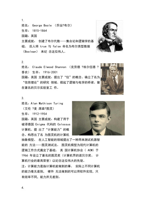
1.姓名：George Boole （乔治?布尔）生卒：1815-1864国籍：英国主要成就：创建了布尔代数——集合论和逻辑学的基础。

后人将true 与false 命名为布尔类型数据（Boolean）来纪念这位伟人。

2.姓名：Claude Elwood Shannon （克劳德?埃尔伍德?香农）生卒：1916-2001国籍：美国主要成就：提出了“位”的概念、确立了名为“信息理论”的研究领域、搭起了逻辑与电学的桥梁。

曾在著名的贝尔实验室工作。

3.姓名：Alan Mathison Turing（艾伦?麦席森?图灵）生卒：1912-1954国籍：英国主要成就：构建了用于破译德国Enigma 代码的Colossus计算机、提出了“计算能力”的概念、构思出了名为图灵机的计算机抽象模型、在人工智能的领域提出了一种用来测试机器智能的方法——图灵测试法。

图灵机模型为现代计算机的逻辑工作方式奠定了基础。

美国计算机协会（ACM）于1966 年设立了著名的图灵奖（计算机界的诺贝尔奖、计算机行业的最高荣誉）以纪念这位伟大的先驱。

注：计算能力是指计算机能做到的事。

实际上不同计算机的能力毫无差别，硬件无法做到的可以用软件实现，只有效率不同，能力并无差别。

4.姓名：Charles Babbage（查尔斯?巴贝奇）生卒：1792-1871国籍：英国主要成就：被誉为计算机的先驱、计算机革命先驱，构想了差分机、解析机。

解析机用卡片编程，设计理念同现代计算机极为相似，可以说在当时又着超越时代的认知，虽然从未完成过，但是其理念对后世影响深远。

5.姓名：Joseph Marie Jacquard（约瑟夫?玛丽?雅卡尔）生卒：1752-1834 国籍：法国主要成就：发明了自动织布机，奠定了后来卡片编程的基础6.姓名：Blaise Pasca（l 布莱斯?帕斯卡）生卒：1623-1662国籍：法国主要成就：1642 年他设计并制作了一台能自动进位的加减法计算装置，被称为是世界上第一台数字计算器，为以后的计算机设计提供了基本原理。

英语发展史_教学课件 Part 1Early_Modern_English_2

(1608-1674)
1633 King James English trading posts
established in Bengal.
1637 English traders established in
Canton.
1639 English established at Madras.
1640 Twenty-four pamphlets were
Pilgrim’s Progress. / Dryden published his greatest play: All for Love.
1679 Parliament dismissed; Charles II
rejected petitions calling for a new Parliament; petitioners became known as Whigs; their opponents (royalists) known as Tories.
Bengal
Ben Jonson
(1572-1637)
The Civil War
1646 English occupied the Bahamas.
1648 Second Civil War.
1649 Charles I beheaded.
Commonwealth established.
1651 Thomas Hobbes published his
outbreak of bubonic plague in England.
The Royal Society
1666 The great fire of London.
New Amsterdam
1667 John Milton, the greatest of English

公共政策终结理论研究综述

公共政策终结理论研究综述摘要：政策终结是政策过程的一个环节，是政策更新、政策发展、政策进步的新起点。

政策终结是20世纪70年代末西方公共政策研究领域的热点问题。

公共政策终结是公共政策过程的一个重要阶段，对政策终结的研究不仅有利于促进政策资源的合理配置，更有利于提高政府的政策绩效。

本文简要回顾了公共政策终结研究的缘起、内涵、类型、方式、影响因素、促成策略以及发展方向等内容，希望能够对公共政策终结理论有一个比较全面深入的了解。

关键词：公共政策，政策终结，理论研究行政有着古老的历史，但是，在一个相当长的历史时期中，行政所赖以治理社会的工具主要是行政行为。

即使是公共行政出现之后，在一个较长的时期内也还主要是借助于行政行为去开展社会治理，公共行政与传统行政的区别在于，找到了行政行为一致性的制度模式，确立了行政行为的（官僚制）组织基础。

到了公共行政的成熟阶段，公共政策作为社会治理的一个重要途径引起了人们的重视。

与传统社会中主要通过行政行为进行社会治理相比，公共政策在解决社会问题、降低社会成本、调节社会运行等方面都显示出了巨大的优势。

但是，如果一项政策已经失去了存在的价值而又继续被保留下来了，就可能会发挥极其消极的作用。

因此，及时、有效地终结一项或一系列错误的或没有价值的公共政策，有利于促进公共政策的更新与发展、推进公共政策的周期性循环、缓解和解决公共政策的矛盾和冲突，从而实现优化和调整公共政策系统的目标。

这就引发了学界对政策终结理论的思考和探索。

自政策科学在美国诞生以来，公共政策过程理论都是学术界所关注的热点。

1956年，拉斯韦尔在《决策过程》一书中提出了决策过程的七个阶段，即情报、建议、规定、行使、运用、评价和终止。

此种观点奠定了政策过程阶段论在公共政策研究中的主导地位。

一时间，对于政策过程各个阶段的研究成为政策学界的主要课题。

然而，相对于其他几个阶段的研究来说，政策终结的研究一直显得非常滞后。

这种情况直到20世纪70年代末80年代初，才有了明显的改善。

美英报刊Lessons 10 Reining In the Test of Tests

Reining In the Test of TestsSome say the SAT is destiny. Some say it'smeaningless.Should it be scrapped?By Ben WildavskyRichard Atkinson is not typical of those who fret over the SAT, yet there he was last year poring over a stack of prep manuals, filling in the bubbles with his No.2 pencils. When the esteemed cognitive psychologist, former head of the National Science Foundation and now president of the prestigious nine-campus University of California system, decided to investigate his long-standing misgivings about the nation's best known standardized test, he did just what many of the 1.3 million high school seniors who take the SAT do every year. Every night or so for several weeks, the 71-year-old Atkinson pulled out his manuals and sample tests to review and assess the sort of verbal and mathematical questions teenagers are up against.理查德·阿特金森(Richard Atkinson)并不是那些为SAT而烦恼的人的典型代表，但去年他在那里钻研着一叠准备手册，用2号铅笔做题。

1_男生英文名大全

Adam，[ˈædəm] 亚当，希伯来天下第一个男人，男性Alan，['ælən] 艾伦，英俊的，好看的；和睦，和平；高兴的。

Albert，['ælbət] 艾伯特英国，高贵的聪明；人类的守护者。

Alexander，[,ælig'za:ndə] 亚历山大，希腊，人类的保护者；Alfred，['ælfrid] 亚尔弗列得，英国；条顿，睿智的顾问；聪明帮手。

Allen，['ælən] 艾伦，盖尔，和谐融洽；英俊的；好看的。

Andrew，['ændru:] 安德鲁希腊，男性的，勇敢的，骁勇的。

Andy，['ændi]安迪，希腊，男性的，勇敢的，骁勇的。

Angelo，['ændʒiləu] 安其罗义大利上帝的使者。

Antony，['æntəni] 安东尼拉丁，值得赞美，备受尊崇的。

Arnold，['ɑ:nəld]阿诺德条顿，鹰。

Arthur，['ɑ:θə] 亚瑟，英国，高尚的或贵族的。

August，[ɔ:ˈgʌst] 奥格斯格，拉丁，神圣的或身份高尚的人；八月。

Augustine，[ɔ:'gʌstin] 奥古斯汀，拉丁，指八月出生的人。

Avery，['eivəri]艾富里英国，争斗；淘气，爱恶作剧的人。

Abraham['eibrə,hæm] 亚伯拉罕Adrian['eidriən] 艾德里安Alva['ælvə] 阿尔瓦Alex['ælɪks] 亚历克斯 (Alexander的昵称)Angus['æŋgəs]安格斯Apollo[ə'pɒləʊ] 阿波罗Austin['ɔ:stin] 奥斯汀Bard，[bɑːd] 巴德，英国，很快乐，且喜欢养家畜的人。

外国人名大全男名

外国人名大全男名Aron 亚伦Abel 亚伯；阿贝尔Abner 艾布纳Abraham 亚伯拉罕（昵称：Abe）Achates 阿凯提斯（忠实的朋友）Adam 亚当Adelbert 阿德尔伯特Adolph 阿道夫Adonis 阿多尼斯（美少年）Adrian 艾德里安Alban 奥尔本Albert 艾尔伯特（昵称：Al, Bert）Alexander 亚历山大（昵称：Aleck, Alex, Sandy）Alexis 亚历克西斯Alfred 艾尔弗雷德（昵称：Al, Alf, Fred）Algernon 阿尔杰农（昵称：Algie, Algy）Allan 阿伦Allen 艾伦Aloysius 阿洛伊修斯Alphonso 阿方索Alvah, Alva 阿尔瓦Alvin 阿尔文Ambrose 安布罗斯Amos 阿莫斯Andrew 安德鲁（昵称：Andy）Angus 安格斯Anthony 安东尼（昵称：T ony）Archibald 阿奇博尔德（昵称：Archie）Arnold 阿诺德Arthur 亚瑟Asa 阿萨August 奥古斯特Augustine 奥古斯丁Augustus 奥古斯都；奥古斯塔斯Austin 奥斯汀Baldwin 鲍德温Barnaby 巴纳比Barnard 巴纳德Bartholomew 巴托洛缪（昵称：Bart）Benedict 本尼迪克特Benjamin 本杰明（昵称：Ben, Benny）Bennett 贝内特Bernard 伯纳德（昵称：Bernie）Bertram 伯特伦（昵称：Bertie）Bertrand 伯特兰Bill 比尔（昵称：Billy）Boris 鲍里斯Brian 布赖恩Bruce 布鲁斯Bruno 布鲁诺Bryan 布莱恩Byron 拜伦Caesar 凯撒Caleb 凯莱布Calvin 卡尔文Cecil 塞西尔Christophe 克里斯托弗Clare 克莱尔Clarence 克拉伦斯Claude 克劳德Clement 克莱门特（昵称：Clem）Clifford 克利福德（昵称：Cliff）Clifton 克利夫顿Clinton 克林顿Clive 克莱夫Clyde 克莱德Colin 科林Conan 科南Conrad 康拉德Cornelius 科尼利厄斯Crispin 克利斯平Curtis 柯蒂斯Cuthbert 卡斯伯特Cyril 西里尔Cyrus 赛勒斯（昵称：Cy）David 大卫；戴维（昵称：Dave, Davy）Denis, Dennis 丹尼斯Dominic 多米尼克Donald 唐纳德（昵称：Don）Douglas 道格拉斯（昵称：Doug）Dudley 达德利Duncan 邓肯Dwight 德怀特Earl, Earle 厄尔Earnest 欧内斯特Ebenezer 欧贝尼泽Edgar 埃德加（昵称：Ed, Ned）Edward 爱德华（昵称：Ed, Ned）Edwin 埃德温（昵称：Ed）Egbert 艾格伯特Elbert 埃尔博特Eli 伊莱Elias 伊莱亚斯Elihu 伊莱休Elijah 伊莱贾（昵称：Lige）Eliot 埃利奥特Elisha 伊莱沙（昵称：Lish）Elliot, Elliott 埃利奥特Ellis 埃利斯Elmer 艾尔默Emery, Emory 艾默里Emil 埃米尔Emmanuel 伊曼纽尔Enoch 伊诺克Enos 伊诺思Ephraim 伊弗雷姆Erasmus 伊拉兹马斯Erastus 伊拉斯塔斯Eric 埃里克Ernest 欧内斯特（昵称：Errie）Erwin 欧文Essex 埃塞克斯（埃塞克斯伯爵，英国军人和廷臣，因叛国罪被处死）Ethan 伊桑Ethelbert 埃塞尔伯特Eugene 尤金（昵称：Gene）Eurus 欧罗斯（东风神或东南风神）Eustace 尤斯塔斯Evan 埃文，伊万Evelyn 伊夫林Everett 埃弗雷特Ezakiel 伊齐基尔（昵称：Zeke）Ezra 埃兹拉Felix 菲利克斯Ferdinand 费迪南德Finlay, Finley 芬利Floyd 弗洛伊德Francis 弗朗西斯（昵称：Frank）Frank 弗兰克Franklin 富兰克林Frederick 弗雷德里克（昵称：Fred）Gabriel 加布里埃尔（昵称：Gabe）Gail 盖尔Gamaliel 甘梅利尔Gary 加里George 乔治Gerald 杰拉尔德Gerard 杰勒德Gideon 吉迪恩Gifford 吉福德Gilbert 吉尔伯特Giles 加尔斯Glenn, Glen 格伦Godfrey 戈弗雷Gordon 戈登Gregory 格雷戈里（昵称：Greg）Griffith 格里菲斯Gustavus 古斯塔夫斯Guthrie 格思里Guy 盖伊Hans 汉斯Harlan 哈伦Harold 哈罗德（昵称：Hal）Harry 哈里Harvey 哈维Hector 赫克托Henry 亨利（昵称：Hal, Hank, Henny）Herbert 赫伯特（昵称：Herb, Bert）Herman 赫尔曼Hilary 希拉里Hiram 海勒姆（昵称：Hi）Homer 霍默Horace 霍勒斯Horatio 霍雷肖Hosea 霍奇亚Howard 霍华德Hubert 休伯特Hugh 休Hugo 雨果Humphrey 汉弗莱Ichabod 伊卡伯德Ignatius 伊格内修斯Immanuel 伊曼纽尔Ira 艾拉Irene 艾林Irving, Irwin 欧文Isaac 艾萨克（昵称：Ike）Isador, Isadore 伊萨多Isaiah 埃塞亚Isidore, Isidor 伊西多（昵称：Izzy）Islington 伊斯林顿Israel 伊斯雷尔（昵称：Izzy）Ivan 伊凡Jack 杰克Jackson 杰克逊Jacob 雅各布（昵称：Jack, Jake）James 詹姆斯（昵称：Jamie, Jim, Jimmy）Jared 贾雷德Jarvis 贾维斯Jason 贾森Jasper 加斯珀Jean 琼Jeffrey 杰弗里（昵称：Jeff）Jeremiah 杰里迈亚（昵称：Jerry）Jeremy 杰里米Jerome 杰罗姆（昵称：Jerry）Jervis 杰维斯Jesse 杰西（昵称：Jess）Jesus 杰苏斯Jim 吉姆Joab 乔巴Job 乔布Joe 乔Joel 乔尔John 约翰（昵称：Jack, Johnnie, Johnny）Jonah 乔纳Jonathan 乔纳森（昵称：Jon）Joseph 约瑟夫（昵称：Joe, Jo）Joshua 乔舒亚（昵称：Josh）Josephus 约瑟夫斯Josiah 乔塞亚Judah 朱达（昵称：Jude）Jude 朱达Jules 朱尔斯Julian 朱利安（昵称：Jule）Julius 朱利叶斯（昵称：Jule, Julie）Junius 朱尼厄斯Justin 贾斯丁Justus 贾斯特斯Keith 基斯Kelvin 凯尔文Kenneth 肯尼斯（昵称：Ken）Kevin 凯文Kit 基特Larry 拉里Laurence, Lawrence 劳伦斯（昵称：Larry）Lazarus 拉扎勒斯Leander 利安德Lee 李Leif 利夫Leigh 李，利Lemuel 莱缪艾尔（昵称：Lem）Leo 利奥Leon 利昂Leonard 列奥纳多（昵称：Len, Lenny）Leopold 利奥波德Leroy 勒鲁瓦Leslie 莱斯利Lester 莱斯特（昵称：Les）Levi 利瓦伊（昵称：Lev）Lewis 刘易斯（昵称：Lew, Lewie）Lionel 莱昂内尔Lewellyn 卢埃林Loyd 劳埃德Lorenzo 洛伦佐Louis 路易斯（昵称：Lou, Louie）Lucian 卢西恩Lucius 卢修斯Luke 卢克Luther 卢瑟Lyman 莱曼Lynn 林恩Manuel 曼纽尔Marcel 马赛尔Marcellus 马塞勒斯Marcus 马库斯Marion 马里恩Mark 马克Marshal 马歇尔Martin 马丁Matthew 马修（昵称：Mat, Matt）Maurice 莫里斯Max 马克斯Maximilian 马克西米利安（昵称：Max）Maynard 梅纳德Melville 梅尔维尔Melvin 梅尔文Merle 莫尔Merlin 莫林Mervin 莫文Micah 迈卡Michael 迈克尔（昵称：Mike, Mickey）Miles 迈尔斯Milton 米尔顿（昵称：Milt, Miltie）Morgan 摩根Morton 莫顿（昵称：Mort, Morty）Moses 摩西（昵称：Mo, Mose）Murray 默里Myron 米隆Nathan 内森（昵称：Nat, Nate）Nathanael 纳撒尼尔Neal,Neil 尼尔Ned 内德Nelson 纳尼森Nestor 涅斯托尔Nicholas, Nicolas 尼古拉斯Nick 尼克Noah 诺亚Noel 诺埃尔Norman 诺曼Octavius 屋大维Oliver 奥利弗Orlando 奥兰多Orson 奥森Orville 奥维尔Oscar 奥斯卡Oswald, Oswold 奥斯瓦尔德Otis 奥蒂斯Otto 奥拓Owen 欧英Patrick 帕特里克（昵称：Paddy, Pat）Paul 保罗Perceval, Percival 帕西瓦尔（昵称：Percy）Percy 珀西Perry 佩里Peter 彼得（昵称：Pete）Philip, Phillip 菲利普（昵称：Phil）Phineas 菲尼亚斯Pierre 皮埃尔Quentin, Quintin 昆廷Ralph 拉尔夫Randal, Randall 兰德尔Randolph 兰道夫Raphael 拉斐尔Raymond 雷蒙德（昵称：Ray）Reginald 雷金纳德Reubin 鲁本Rex 雷克斯Richard 理查德Robert 罗伯特Rodney 罗德尼Roger 罗杰Roland, Rowland 罗兰Rolf 罗尔夫Ronald 罗纳德Roscoe 罗斯科Rudolph 鲁道夫Rufus 鲁弗斯Rupert 鲁珀特Russell, Russel 罗素Sammy 萨米Sam 萨姆Samson 萨姆森Samuel 塞缪尔Saul 索尔Seth 赛思Seymour 西摩尔Sidney 西德尼Sigmund 西格蒙德Silas 塞拉斯Silvester 西尔维斯特Simeon 西米恩Simon 西蒙Solomon 所罗门（昵称：Sol）Stanley 斯坦利Stephen 斯蒂芬Steven 史蒂文Stewart, Stuart 斯图尔特Sydney 西德尼Sylvanus 西尔韦纳斯Sylvester 西尔威斯特Terence 特伦斯（昵称：Terry）Thaddeus, Thadeus 萨迪厄斯Theobald 西奥波尔德Theodore 西奥多Theodosius 西奥多西Thomas 托马斯（昵称：Tom, Tommy）Timothy 蒂莫西（昵称：Tim）Titus 泰特斯Tobiah 托比厄（昵称：Toby）Tony 托尼Tristram 特里斯托拉姆（昵称：Tris）Uriah 尤赖亚Valentine 瓦伦丁Vernon 弗农Victor 维克托（昵称：Vic）Vincent 文森特Virgil 弗吉尔Waldo 沃尔多Wallace 华莱士（昵称：Wally）Walter 沃尔特（昵称：Walt, Wat）Warren 沃伦Wayne 韦恩Wesley 韦斯利Wilbert 威尔伯特Wilbur 威尔伯Wilfred, Wilfrid 威尔弗雷德Willard 威拉德William 威廉（昵称：Will, Willy）Willis 威利斯Winfred 温弗雷德Woodrow 伍德罗（昵称：Woody）Zachariah 扎卡赖亚（昵称：Zach）Zacharias 扎卡赖亚斯Zachary 扎卡里Zebulun 泽布伦。

《神经网络与深度学习综述DeepLearning15May2014

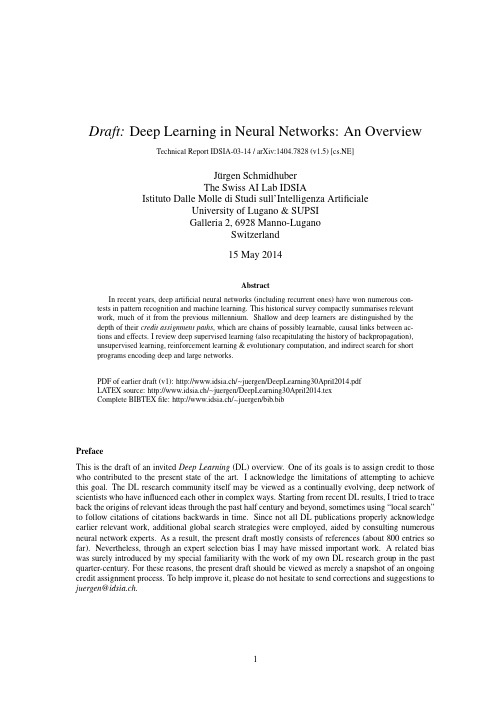
Draft:Deep Learning in Neural Networks:An OverviewTechnical Report IDSIA-03-14/arXiv:1404.7828(v1.5)[cs.NE]J¨u rgen SchmidhuberThe Swiss AI Lab IDSIAIstituto Dalle Molle di Studi sull’Intelligenza ArtiﬁcialeUniversity of Lugano&SUPSIGalleria2,6928Manno-LuganoSwitzerland15May2014AbstractIn recent years,deep artiﬁcial neural networks(including recurrent ones)have won numerous con-tests in pattern recognition and machine learning.This historical survey compactly summarises relevantwork,much of it from the previous millennium.Shallow and deep learners are distinguished by thedepth of their credit assignment paths,which are chains of possibly learnable,causal links between ac-tions and effects.I review deep supervised learning(also recapitulating the history of backpropagation),unsupervised learning,reinforcement learning&evolutionary computation,and indirect search for shortprograms encoding deep and large networks.PDF of earlier draft(v1):http://www.idsia.ch/∼juergen/DeepLearning30April2014.pdfLATEX source:http://www.idsia.ch/∼juergen/DeepLearning30April2014.texComplete BIBTEXﬁle:http://www.idsia.ch/∼juergen/bib.bibPrefaceThis is the draft of an invited Deep Learning(DL)overview.One of its goals is to assign credit to those who contributed to the present state of the art.I acknowledge the limitations of attempting to achieve this goal.The DL research community itself may be viewed as a continually evolving,deep network of scientists who have inﬂuenced each other in complex ways.Starting from recent DL results,I tried to trace back the origins of relevant ideas through the past half century and beyond,sometimes using“local search”to follow citations of citations backwards in time.Since not all DL publications properly acknowledge earlier relevant work,additional global search strategies were employed,aided by consulting numerous neural network experts.As a result,the present draft mostly consists of references(about800entries so far).Nevertheless,through an expert selection bias I may have missed important work.A related bias was surely introduced by my special familiarity with the work of my own DL research group in the past quarter-century.For these reasons,the present draft should be viewed as merely a snapshot of an ongoing credit assignment process.To help improve it,please do not hesitate to send corrections and suggestions to juergen@idsia.ch.Contents1Introduction to Deep Learning(DL)in Neural Networks(NNs)3 2Event-Oriented Notation for Activation Spreading in FNNs/RNNs3 3Depth of Credit Assignment Paths(CAPs)and of Problems4 4Recurring Themes of Deep Learning54.1Dynamic Programming(DP)for DL (5)4.2Unsupervised Learning(UL)Facilitating Supervised Learning(SL)and RL (6)4.3Occam’s Razor:Compression and Minimum Description Length(MDL) (6)4.4Learning Hierarchical Representations Through Deep SL,UL,RL (6)4.5Fast Graphics Processing Units(GPUs)for DL in NNs (6)5Supervised NNs,Some Helped by Unsupervised NNs75.11940s and Earlier (7)5.2Around1960:More Neurobiological Inspiration for DL (7)5.31965:Deep Networks Based on the Group Method of Data Handling(GMDH) (8)5.41979:Convolution+Weight Replication+Winner-Take-All(WTA) (8)5.51960-1981and Beyond:Development of Backpropagation(BP)for NNs (8)5.5.1BP for Weight-Sharing Feedforward NNs(FNNs)and Recurrent NNs(RNNs)..95.6Late1980s-2000:Numerous Improvements of NNs (9)5.6.1Ideas for Dealing with Long Time Lags and Deep CAPs (10)5.6.2Better BP Through Advanced Gradient Descent (10)5.6.3Discovering Low-Complexity,Problem-Solving NNs (11)5.6.4Potential Beneﬁts of UL for SL (11)5.71987:UL Through Autoencoder(AE)Hierarchies (12)5.81989:BP for Convolutional NNs(CNNs) (13)5.91991:Fundamental Deep Learning Problem of Gradient Descent (13)5.101991:UL-Based History Compression Through a Deep Hierarchy of RNNs (14)5.111992:Max-Pooling(MP):Towards MPCNNs (14)5.121994:Contest-Winning Not So Deep NNs (15)5.131995:Supervised Recurrent Very Deep Learner(LSTM RNN) (15)5.142003:More Contest-Winning/Record-Setting,Often Not So Deep NNs (16)5.152006/7:Deep Belief Networks(DBNs)&AE Stacks Fine-Tuned by BP (17)5.162006/7:Improved CNNs/GPU-CNNs/BP-Trained MPCNNs (17)5.172009:First Ofﬁcial Competitions Won by RNNs,and with MPCNNs (18)5.182010:Plain Backprop(+Distortions)on GPU Yields Excellent Results (18)5.192011:MPCNNs on GPU Achieve Superhuman Vision Performance (18)5.202011:Hessian-Free Optimization for RNNs (19)5.212012:First Contests Won on ImageNet&Object Detection&Segmentation (19)5.222013-:More Contests and Benchmark Records (20)5.22.1Currently Successful Supervised Techniques:LSTM RNNs/GPU-MPCNNs (21)5.23Recent Tricks for Improving SL Deep NNs(Compare Sec.5.6.2,5.6.3) (21)5.24Consequences for Neuroscience (22)5.25DL with Spiking Neurons? (22)6DL in FNNs and RNNs for Reinforcement Learning(RL)236.1RL Through NN World Models Yields RNNs With Deep CAPs (23)6.2Deep FNNs for Traditional RL and Markov Decision Processes(MDPs) (24)6.3Deep RL RNNs for Partially Observable MDPs(POMDPs) (24)6.4RL Facilitated by Deep UL in FNNs and RNNs (25)6.5Deep Hierarchical RL(HRL)and Subgoal Learning with FNNs and RNNs (25)6.6Deep RL by Direct NN Search/Policy Gradients/Evolution (25)6.7Deep RL by Indirect Policy Search/Compressed NN Search (26)6.8Universal RL (27)7Conclusion271Introduction to Deep Learning(DL)in Neural Networks(NNs) Which modiﬁable components of a learning system are responsible for its success or failure?What changes to them improve performance?This has been called the fundamental credit assignment problem(Minsky, 1963).There are general credit assignment methods for universal problem solvers that are time-optimal in various theoretical senses(Sec.6.8).The present survey,however,will focus on the narrower,but now commercially important,subﬁeld of Deep Learning(DL)in Artiﬁcial Neural Networks(NNs).We are interested in accurate credit assignment across possibly many,often nonlinear,computational stages of NNs.Shallow NN-like models have been around for many decades if not centuries(Sec.5.1).Models with several successive nonlinear layers of neurons date back at least to the1960s(Sec.5.3)and1970s(Sec.5.5). An efﬁcient gradient descent method for teacher-based Supervised Learning(SL)in discrete,differentiable networks of arbitrary depth called backpropagation(BP)was developed in the1960s and1970s,and ap-plied to NNs in1981(Sec.5.5).BP-based training of deep NNs with many layers,however,had been found to be difﬁcult in practice by the late1980s(Sec.5.6),and had become an explicit research subject by the early1990s(Sec.5.9).DL became practically feasible to some extent through the help of Unsupervised Learning(UL)(e.g.,Sec.5.10,5.15).The1990s and2000s also saw many improvements of purely super-vised DL(Sec.5).In the new millennium,deep NNs haveﬁnally attracted wide-spread attention,mainly by outperforming alternative machine learning methods such as kernel machines(Vapnik,1995;Sch¨o lkopf et al.,1998)in numerous important applications.In fact,supervised deep NNs have won numerous of-ﬁcial international pattern recognition competitions(e.g.,Sec.5.17,5.19,5.21,5.22),achieving theﬁrst superhuman visual pattern recognition results in limited domains(Sec.5.19).Deep NNs also have become relevant for the more generalﬁeld of Reinforcement Learning(RL)where there is no supervising teacher (Sec.6).Both feedforward(acyclic)NNs(FNNs)and recurrent(cyclic)NNs(RNNs)have won contests(Sec.5.12,5.14,5.17,5.19,5.21,5.22).In a sense,RNNs are the deepest of all NNs(Sec.3)—they are general computers more powerful than FNNs,and can in principle create and process memories of ar-bitrary sequences of input patterns(e.g.,Siegelmann and Sontag,1991;Schmidhuber,1990a).Unlike traditional methods for automatic sequential program synthesis(e.g.,Waldinger and Lee,1969;Balzer, 1985;Soloway,1986;Deville and Lau,1994),RNNs can learn programs that mix sequential and parallel information processing in a natural and efﬁcient way,exploiting the massive parallelism viewed as crucial for sustaining the rapid decline of computation cost observed over the past75years.The rest of this paper is structured as follows.Sec.2introduces a compact,event-oriented notation that is simple yet general enough to accommodate both FNNs and RNNs.Sec.3introduces the concept of Credit Assignment Paths(CAPs)to measure whether learning in a given NN application is of the deep or shallow type.Sec.4lists recurring themes of DL in SL,UL,and RL.Sec.5focuses on SL and UL,and on how UL can facilitate SL,although pure SL has become dominant in recent competitions(Sec.5.17-5.22). Sec.5is arranged in a historical timeline format with subsections on important inspirations and technical contributions.Sec.6on deep RL discusses traditional Dynamic Programming(DP)-based RL combined with gradient-based search techniques for SL or UL in deep NNs,as well as general methods for direct and indirect search in the weight space of deep FNNs and RNNs,including successful policy gradient and evolutionary methods.2Event-Oriented Notation for Activation Spreading in FNNs/RNNs Throughout this paper,let i,j,k,t,p,q,r denote positive integer variables assuming ranges implicit in the given contexts.Let n,m,T denote positive integer constants.An NN’s topology may change over time(e.g.,Fahlman,1991;Ring,1991;Weng et al.,1992;Fritzke, 1994).At any given moment,it can be described as aﬁnite subset of units(or nodes or neurons)N= {u1,u2,...,}and aﬁnite set H⊆N×N of directed edges or connections between nodes.FNNs are acyclic graphs,RNNs cyclic.Theﬁrst(input)layer is the set of input units,a subset of N.In FNNs,the k-th layer(k>1)is the set of all nodes u∈N such that there is an edge path of length k−1(but no longer path)between some input unit and u.There may be shortcut connections between distant layers.The NN’s behavior or program is determined by a set of real-valued,possibly modiﬁable,parameters or weights w i(i=1,...,n).We now focus on a singleﬁnite episode or epoch of information processing and activation spreading,without learning through weight changes.The following slightly unconventional notation is designed to compactly describe what is happening during the runtime of the system.During an episode,there is a partially causal sequence x t(t=1,...,T)of real values that I call events.Each x t is either an input set by the environment,or the activation of a unit that may directly depend on other x k(k<t)through a current NN topology-dependent set in t of indices k representing incoming causal connections or links.Let the function v encode topology information and map such event index pairs(k,t)to weight indices.For example,in the non-input case we may have x t=f t(net t)with real-valued net t= k∈in t x k w v(k,t)(additive case)or net t= k∈in t x k w v(k,t)(multiplicative case), where f t is a typically nonlinear real-valued activation function such as tanh.In many recent competition-winning NNs(Sec.5.19,5.21,5.22)there also are events of the type x t=max k∈int (x k);some networktypes may also use complex polynomial activation functions(Sec.5.3).x t may directly affect certain x k(k>t)through outgoing connections or links represented through a current set out t of indices k with t∈in k.Some non-input events are called output events.Note that many of the x t may refer to different,time-varying activations of the same unit in sequence-processing RNNs(e.g.,Williams,1989,“unfolding in time”),or also in FNNs sequentially exposed to time-varying input patterns of a large training set encoded as input events.During an episode,the same weight may get reused over and over again in topology-dependent ways,e.g.,in RNNs,or in convolutional NNs(Sec.5.4,5.8).I call this weight sharing across space and/or time.Weight sharing may greatly reduce the NN’s descriptive complexity,which is the number of bits of information required to describe the NN (Sec.4.3).In Supervised Learning(SL),certain NN output events x t may be associated with teacher-given,real-valued labels or targets d t yielding errors e t,e.g.,e t=1/2(x t−d t)2.A typical goal of supervised NN training is toﬁnd weights that yield episodes with small total error E,the sum of all such e t.The hope is that the NN will generalize well in later episodes,causing only small errors on previously unseen sequences of input events.Many alternative error functions for SL and UL are possible.SL assumes that input events are independent of earlier output events(which may affect the environ-ment through actions causing subsequent perceptions).This assumption does not hold in the broaderﬁelds of Sequential Decision Making and Reinforcement Learning(RL)(Kaelbling et al.,1996;Sutton and Barto, 1998;Hutter,2005)(Sec.6).In RL,some of the input events may encode real-valued reward signals given by the environment,and a typical goal is toﬁnd weights that yield episodes with a high sum of reward signals,through sequences of appropriate output actions.Sec.5.5will use the notation above to compactly describe a central algorithm of DL,namely,back-propagation(BP)for supervised weight-sharing FNNs and RNNs.(FNNs may be viewed as RNNs with certainﬁxed zero weights.)Sec.6will address the more general RL case.3Depth of Credit Assignment Paths(CAPs)and of ProblemsTo measure whether credit assignment in a given NN application is of the deep or shallow type,I introduce the concept of Credit Assignment Paths or CAPs,which are chains of possibly causal links between events.Let usﬁrst focus on SL.Consider two events x p and x q(1≤p<q≤T).Depending on the appli-cation,they may have a Potential Direct Causal Connection(PDCC)expressed by the Boolean predicate pdcc(p,q),which is true if and only if p∈in q.Then the2-element list(p,q)is deﬁned to be a CAP from p to q(a minimal one).A learning algorithm may be allowed to change w v(p,q)to improve performance in future episodes.More general,possibly indirect,Potential Causal Connections(PCC)are expressed by the recursively deﬁned Boolean predicate pcc(p,q),which in the SL case is true only if pdcc(p,q),or if pcc(p,k)for some k and pdcc(k,q).In the latter case,appending q to any CAP from p to k yields a CAP from p to q(this is a recursive deﬁnition,too).The set of such CAPs may be large but isﬁnite.Note that the same weight may affect many different PDCCs between successive events listed by a given CAP,e.g.,in the case of RNNs, or weight-sharing FNNs.Suppose a CAP has the form(...,k,t,...,q),where k and t(possibly t=q)are theﬁrst successive elements with modiﬁable w v(k,t).Then the length of the sufﬁx list(t,...,q)is called the CAP’s depth (which is0if there are no modiﬁable links at all).This depth limits how far backwards credit assignment can move down the causal chain toﬁnd a modiﬁable weight.1Suppose an episode and its event sequence x1,...,x T satisfy a computable criterion used to decide whether a given problem has been solved(e.g.,total error E below some threshold).Then the set of used weights is called a solution to the problem,and the depth of the deepest CAP within the sequence is called the solution’s depth.There may be other solutions(yielding different event sequences)with different depths.Given someﬁxed NN topology,the smallest depth of any solution is called the problem’s depth.Sometimes we also speak of the depth of an architecture:SL FNNs withﬁxed topology imply a problem-independent maximal problem depth bounded by the number of non-input layers.Certain SL RNNs withﬁxed weights for all connections except those to output units(Jaeger,2001;Maass et al.,2002; Jaeger,2004;Schrauwen et al.,2007)have a maximal problem depth of1,because only theﬁnal links in the corresponding CAPs are modiﬁable.In general,however,RNNs may learn to solve problems of potentially unlimited depth.Note that the deﬁnitions above are solely based on the depths of causal chains,and agnostic of the temporal distance between events.For example,shallow FNNs perceiving large“time windows”of in-put events may correctly classify long input sequences through appropriate output events,and thus solve shallow problems involving long time lags between relevant events.At which problem depth does Shallow Learning end,and Deep Learning begin?Discussions with DL experts have not yet yielded a conclusive response to this question.Instead of committing myself to a precise answer,let me just deﬁne for the purposes of this overview:problems of depth>10require Very Deep Learning.The difﬁculty of a problem may have little to do with its depth.Some NNs can quickly learn to solve certain deep problems,e.g.,through random weight guessing(Sec.5.9)or other types of direct search (Sec.6.6)or indirect search(Sec.6.7)in weight space,or through training an NNﬁrst on shallow problems whose solutions may then generalize to deep problems,or through collapsing sequences of(non)linear operations into a single(non)linear operation—but see an analysis of non-trivial aspects of deep linear networks(Baldi and Hornik,1994,Section B).In general,however,ﬁnding an NN that precisely models a given training set is an NP-complete problem(Judd,1990;Blum and Rivest,1992),also in the case of deep NNs(S´ıma,1994;de Souto et al.,1999;Windisch,2005);compare a survey of negative results(S´ıma, 2002,Section1).Above we have focused on SL.In the more general case of RL in unknown environments,pcc(p,q) is also true if x p is an output event and x q any later input event—any action may affect the environment and thus any later perception.(In the real world,the environment may even inﬂuence non-input events computed on a physical hardware entangled with the entire universe,but this is ignored here.)It is possible to model and replace such unmodiﬁable environmental PCCs through a part of the NN that has already learned to predict(through some of its units)input events(including reward signals)from former input events and actions(Sec.6.1).Its weights are frozen,but can help to assign credit to other,still modiﬁable weights used to compute actions(Sec.6.1).This approach may lead to very deep CAPs though.Some DL research is about automatically rephrasing problems such that their depth is reduced(Sec.4). In particular,sometimes UL is used to make SL problems less deep,e.g.,Sec.5.10.Often Dynamic Programming(Sec.4.1)is used to facilitate certain traditional RL problems,e.g.,Sec.6.2.Sec.5focuses on CAPs for SL,Sec.6on the more complex case of RL.4Recurring Themes of Deep Learning4.1Dynamic Programming(DP)for DLOne recurring theme of DL is Dynamic Programming(DP)(Bellman,1957),which can help to facili-tate credit assignment under certain assumptions.For example,in SL NNs,backpropagation itself can 1An alternative would be to count only modiﬁable links when measuring depth.In many typical NN applications this would not make a difference,but in some it would,e.g.,Sec.6.1.be viewed as a DP-derived method(Sec.5.5).In traditional RL based on strong Markovian assumptions, DP-derived methods can help to greatly reduce problem depth(Sec.6.2).DP algorithms are also essen-tial for systems that combine concepts of NNs and graphical models,such as Hidden Markov Models (HMMs)(Stratonovich,1960;Baum and Petrie,1966)and Expectation Maximization(EM)(Dempster et al.,1977),e.g.,(Bottou,1991;Bengio,1991;Bourlard and Morgan,1994;Baldi and Chauvin,1996; Jordan and Sejnowski,2001;Bishop,2006;Poon and Domingos,2011;Dahl et al.,2012;Hinton et al., 2012a).4.2Unsupervised Learning(UL)Facilitating Supervised Learning(SL)and RL Another recurring theme is how UL can facilitate both SL(Sec.5)and RL(Sec.6).UL(Sec.5.6.4) is normally used to encode raw incoming data such as video or speech streams in a form that is more convenient for subsequent goal-directed learning.In particular,codes that describe the original data in a less redundant or more compact way can be fed into SL(Sec.5.10,5.15)or RL machines(Sec.6.4),whose search spaces may thus become smaller(and whose CAPs shallower)than those necessary for dealing with the raw data.UL is closely connected to the topics of regularization and compression(Sec.4.3,5.6.3). 4.3Occam’s Razor:Compression and Minimum Description Length(MDL) Occam’s razor favors simple solutions over complex ones.Given some programming language,the prin-ciple of Minimum Description Length(MDL)can be used to measure the complexity of a solution candi-date by the length of the shortest program that computes it(e.g.,Solomonoff,1964;Kolmogorov,1965b; Chaitin,1966;Wallace and Boulton,1968;Levin,1973a;Rissanen,1986;Blumer et al.,1987;Li and Vit´a nyi,1997;Gr¨u nwald et al.,2005).Some methods explicitly take into account program runtime(Al-lender,1992;Watanabe,1992;Schmidhuber,2002,1995);many consider only programs with constant runtime,written in non-universal programming languages(e.g.,Rissanen,1986;Hinton and van Camp, 1993).In the NN case,the MDL principle suggests that low NN weight complexity corresponds to high NN probability in the Bayesian view(e.g.,MacKay,1992;Buntine and Weigend,1991;De Freitas,2003), and to high generalization performance(e.g.,Baum and Haussler,1989),without overﬁtting the training data.Many methods have been proposed for regularizing NNs,that is,searching for solution-computing, low-complexity SL NNs(Sec.5.6.3)and RL NNs(Sec.6.7).This is closely related to certain UL methods (Sec.4.2,5.6.4).4.4Learning Hierarchical Representations Through Deep SL,UL,RLMany methods of Good Old-Fashioned Artiﬁcial Intelligence(GOFAI)(Nilsson,1980)as well as more recent approaches to AI(Russell et al.,1995)and Machine Learning(Mitchell,1997)learn hierarchies of more and more abstract data representations.For example,certain methods of syntactic pattern recog-nition(Fu,1977)such as grammar induction discover hierarchies of formal rules to model observations. The partially(un)supervised Automated Mathematician/EURISKO(Lenat,1983;Lenat and Brown,1984) continually learns concepts by combining previously learnt concepts.Such hierarchical representation learning(Ring,1994;Bengio et al.,2013;Deng and Yu,2014)is also a recurring theme of DL NNs for SL (Sec.5),UL-aided SL(Sec.5.7,5.10,5.15),and hierarchical RL(Sec.6.5).Often,abstract hierarchical representations are natural by-products of data compression(Sec.4.3),e.g.,Sec.5.10.4.5Fast Graphics Processing Units(GPUs)for DL in NNsWhile the previous millennium saw several attempts at creating fast NN-speciﬁc hardware(e.g.,Jackel et al.,1990;Faggin,1992;Ramacher et al.,1993;Widrow et al.,1994;Heemskerk,1995;Korkin et al., 1997;Urlbe,1999),and at exploiting standard hardware(e.g.,Anguita et al.,1994;Muller et al.,1995; Anguita and Gomes,1996),the new millennium brought a DL breakthrough in form of cheap,multi-processor graphics cards or GPUs.GPUs are widely used for video games,a huge and competitive market that has driven down hardware prices.GPUs excel at fast matrix and vector multiplications required not only for convincing virtual realities but also for NN training,where they can speed up learning by a factorof50and more.Some of the GPU-based FNN implementations(Sec.5.16-5.19)have greatly contributed to recent successes in contests for pattern recognition(Sec.5.19-5.22),image segmentation(Sec.5.21), and object detection(Sec.5.21-5.22).5Supervised NNs,Some Helped by Unsupervised NNsThe main focus of current practical applications is on Supervised Learning(SL),which has dominated re-cent pattern recognition contests(Sec.5.17-5.22).Several methods,however,use additional Unsupervised Learning(UL)to facilitate SL(Sec.5.7,5.10,5.15).It does make sense to treat SL and UL in the same section:often gradient-based methods,such as BP(Sec.5.5.1),are used to optimize objective functions of both UL and SL,and the boundary between SL and UL may blur,for example,when it comes to time series prediction and sequence classiﬁcation,e.g.,Sec.5.10,5.12.A historical timeline format will help to arrange subsections on important inspirations and techni-cal contributions(although such a subsection may span a time interval of many years).Sec.5.1brieﬂy mentions early,shallow NN models since the1940s,Sec.5.2additional early neurobiological inspiration relevant for modern Deep Learning(DL).Sec.5.3is about GMDH networks(since1965),perhaps theﬁrst (feedforward)DL systems.Sec.5.4is about the relatively deep Neocognitron NN(1979)which is similar to certain modern deep FNN architectures,as it combines convolutional NNs(CNNs),weight pattern repli-cation,and winner-take-all(WTA)mechanisms.Sec.5.5uses the notation of Sec.2to compactly describe a central algorithm of DL,namely,backpropagation(BP)for supervised weight-sharing FNNs and RNNs. It also summarizes the history of BP1960-1981and beyond.Sec.5.6describes problems encountered in the late1980s with BP for deep NNs,and mentions several ideas from the previous millennium to overcome them.Sec.5.7discusses aﬁrst hierarchical stack of coupled UL-based Autoencoders(AEs)—this concept resurfaced in the new millennium(Sec.5.15).Sec.5.8is about applying BP to CNNs,which is important for today’s DL applications.Sec.5.9explains BP’s Fundamental DL Problem(of vanishing/exploding gradients)discovered in1991.Sec.5.10explains how a deep RNN stack of1991(the History Compressor) pre-trained by UL helped to solve previously unlearnable DL benchmarks requiring Credit Assignment Paths(CAPs,Sec.3)of depth1000and more.Sec.5.11discusses a particular WTA method called Max-Pooling(MP)important in today’s DL FNNs.Sec.5.12mentions aﬁrst important contest won by SL NNs in1994.Sec.5.13describes a purely supervised DL RNN(Long Short-Term Memory,LSTM)for problems of depth1000and more.Sec.5.14mentions an early contest of2003won by an ensemble of shallow NNs, as well as good pattern recognition results with CNNs and LSTM RNNs(2003).Sec.5.15is mostly about Deep Belief Networks(DBNs,2006)and related stacks of Autoencoders(AEs,Sec.5.7)pre-trained by UL to facilitate BP-based SL.Sec.5.16mentions theﬁrst BP-trained MPCNNs(2007)and GPU-CNNs(2006). Sec.5.17-5.22focus on ofﬁcial competitions with secret test sets won by(mostly purely supervised)DL NNs since2009,in sequence recognition,image classiﬁcation,image segmentation,and object detection. Many RNN results depended on LSTM(Sec.5.13);many FNN results depended on GPU-based FNN code developed since2004(Sec.5.16,5.17,5.18,5.19),in particular,GPU-MPCNNs(Sec.5.19).5.11940s and EarlierNN research started in the1940s(e.g.,McCulloch and Pitts,1943;Hebb,1949);compare also later work on learning NNs(Rosenblatt,1958,1962;Widrow and Hoff,1962;Grossberg,1969;Kohonen,1972; von der Malsburg,1973;Narendra and Thathatchar,1974;Willshaw and von der Malsburg,1976;Palm, 1980;Hopﬁeld,1982).In a sense NNs have been around even longer,since early supervised NNs were essentially variants of linear regression methods going back at least to the early1800s(e.g.,Legendre, 1805;Gauss,1809,1821).Early NNs had a maximal CAP depth of1(Sec.3).5.2Around1960:More Neurobiological Inspiration for DLSimple cells and complex cells were found in the cat’s visual cortex(e.g.,Hubel and Wiesel,1962;Wiesel and Hubel,1959).These cellsﬁre in response to certain properties of visual sensory inputs,such as theorientation of plex cells exhibit more spatial invariance than simple cells.This inspired later deep NN architectures(Sec.5.4)used in certain modern award-winning Deep Learners(Sec.5.19-5.22).5.31965:Deep Networks Based on the Group Method of Data Handling(GMDH) Networks trained by the Group Method of Data Handling(GMDH)(Ivakhnenko and Lapa,1965; Ivakhnenko et al.,1967;Ivakhnenko,1968,1971)were perhaps theﬁrst DL systems of the Feedforward Multilayer Perceptron type.The units of GMDH nets may have polynomial activation functions imple-menting Kolmogorov-Gabor polynomials(more general than traditional NN activation functions).Given a training set,layers are incrementally grown and trained by regression analysis,then pruned with the help of a separate validation set(using today’s terminology),where Decision Regularisation is used to weed out superﬂuous units.The numbers of layers and units per layer can be learned in problem-dependent fashion. This is a good example of hierarchical representation learning(Sec.4.4).There have been numerous ap-plications of GMDH-style networks,e.g.(Ikeda et al.,1976;Farlow,1984;Madala and Ivakhnenko,1994; Ivakhnenko,1995;Kondo,1998;Kord´ık et al.,2003;Witczak et al.,2006;Kondo and Ueno,2008).5.41979:Convolution+Weight Replication+Winner-Take-All(WTA)Apart from deep GMDH networks(Sec.5.3),the Neocognitron(Fukushima,1979,1980,2013a)was per-haps theﬁrst artiﬁcial NN that deserved the attribute deep,and theﬁrst to incorporate the neurophysiolog-ical insights of Sec.5.2.It introduced convolutional NNs(today often called CNNs or convnets),where the(typically rectangular)receptiveﬁeld of a convolutional unit with given weight vector is shifted step by step across a2-dimensional array of input values,such as the pixels of an image.The resulting2D array of subsequent activation events of this unit can then provide inputs to higher-level units,and so on.Due to massive weight replication(Sec.2),relatively few parameters may be necessary to describe the behavior of such a convolutional layer.Competition layers have WTA subsets whose maximally active units are the only ones to adopt non-zero activation values.They essentially“down-sample”the competition layer’s input.This helps to create units whose responses are insensitive to small image shifts(compare Sec.5.2).The Neocognitron is very similar to the architecture of modern,contest-winning,purely super-vised,feedforward,gradient-based Deep Learners with alternating convolutional and competition lay-ers(e.g.,Sec.5.19-5.22).Fukushima,however,did not set the weights by supervised backpropagation (Sec.5.5,5.8),but by local un supervised learning rules(e.g.,Fukushima,2013b),or by pre-wiring.In that sense he did not care for the DL problem(Sec.5.9),although his architecture was comparatively deep indeed.He also used Spatial Averaging(Fukushima,1980,2011)instead of Max-Pooling(MP,Sec.5.11), currently a particularly convenient and popular WTA mechanism.Today’s CNN-based DL machines proﬁta lot from later CNN work(e.g.,LeCun et al.,1989;Ranzato et al.,2007)(Sec.5.8,5.16,5.19).5.51960-1981and Beyond:Development of Backpropagation(BP)for NNsThe minimisation of errors through gradient descent(Hadamard,1908)in the parameter space of com-plex,nonlinear,differentiable,multi-stage,NN-related systems has been discussed at least since the early 1960s(e.g.,Kelley,1960;Bryson,1961;Bryson and Denham,1961;Pontryagin et al.,1961;Dreyfus,1962; Wilkinson,1965;Amari,1967;Bryson and Ho,1969;Director and Rohrer,1969;Griewank,2012),ini-tially within the framework of Euler-LaGrange equations in the Calculus of Variations(e.g.,Euler,1744). Steepest descent in such systems can be performed(Bryson,1961;Kelley,1960;Bryson and Ho,1969)by iterating the ancient chain rule(Leibniz,1676;L’Hˆo pital,1696)in Dynamic Programming(DP)style(Bell-man,1957).A simpliﬁed derivation of the method uses the chain rule only(Dreyfus,1962).The methods of the1960s were already efﬁcient in the DP sense.However,they backpropagated derivative information through standard Jacobian matrix calculations from one“layer”to the previous one, explicitly addressing neither direct links across several layers nor potential additional efﬁciency gains due to network sparsity(but perhaps such enhancements seemed obvious to the authors).。

The_Bullwhip_Effect_in_Supply_Chains

The Bullwhip Effect In Supply Chains1Hau L Lee, V Padmanabhan, and Seungjin Whang;Sloan Management Review, Spring 1997, Volume 38, Issue 3, pp. 93-102 Abstract:The bullwhip effect occurs when the demand order variabilities in the supply chain are amplified as they moved up the supply chain. Distorted information from one end of a supply chain to the other can lead to tremendous inefficiencies. Companies can effectively counteract the bullwhip effect by thoroughly understanding its underlying causes. Industry leaders are implementing innovative strategies that pose new challenges: 1. integrating new information systems, 2. defining new organizational relationships, and 3. implementing new incentive and measurement systems.Distorted information from one end of a supply chain to the other can lead to tremendousinefficiencies: excessive inventory investment, poor customer service, lost revenues, misguided capacity plans, inactive transportation, and missed production schedules. How do exaggeratedorder swings occur? What can companies do to mitigate them?Not long ago, logistics executives at Procter & Gamble (P&G) examined the order patterns for one of their best-selling products, Pampers. Its sales at retail stores were fluctuating, but the variabilities were certainly not excessive. However, as they examined the distributors' orders, the executives were surprised by the degree of variability. When they looked at P&G's orders of materials to their suppliers, such as 3M, they discovered that the swings were even greater. At first glance, the variabilities did not make sense. While the consumers, in this case, the babies, consumed diapers at a steady rate, the demand order variabilities in the supply chain were amplified as they moved up the supply chain. P&G called this phenomenon the "bullwhip" effect. (In some industries, it is known as the "whiplash" or the "whipsaw" effect.)When Hewlett-Packard (HP) executives examined the sales of one of its printers at a major reseller, they found that there were, as expected, some fluctuations over time. However, when they examined the orders from the reseller, they observed much bigger swings. Also, to their surprise, they discovered that the orders from the printer division to the company's integrated circuit division had even greater fluctuations.What happens when a supply chain is plagued with a bullwhip effect that distorts its demand information as it is transmitted up the chain? In the past, without being able to see the sales of its products at the distribution channel stage, HP had to rely on the sales orders from the resellers to make product forecasts, plan capacity, control inventory, and schedule production. Big variations in demand were a major problem for HP's management. The common symptoms of such variations could be excessive inventory, poor product forecasts, insufficient or excessive capacities, poor customer service due to unavailable products or long backlogs, uncertain production planning (i.e., excessive revisions), and high costs for corrections, such as for expedited shipments and overtime. HP's product division was a victim of order swings that were exaggerated by the resellers relative to their sales; it, in turn, created additional exaggerations of order swings to suppliers.In the past few years, the Efficient Consumer Response (ECR) initiative has tried to redefine how the grocery supply chain should work.[1] One motivation for the initiative was the excessive amount of inventory in the supply chain. Various industry studies found that the total supply chain, from when1 Copyright Sloan Management Review Association, Alfred P. Sloan School of Management Spring 1997products leave the manufacturers' production lines to when they arrive on the retailers' shelves, has more than 100 days of inventory supply. Distorted information has led every entity in the supply chain - the plant warehouse, a manufacturer's shuttle warehouse, a manufacturer's market warehouse, a distributor's central warehouse, the distributor's regional warehouses, and the retail store's storage space - to stockpile because of the high degree of demand uncertainties and variabilities. It's no wonder that the ECR reports estimated a potential $30 billion opportunity from streamlining the inefficiencies of the grocery supply chain.[2]Figure 1 Increasing Variability of Orders up the Supply ChainOther industries are in a similar position. Computer factories and manufacturers' distribution centers, the distributors' warehouses, and store warehouses along the distribution channel have inventory stockpiles. And in the pharmaceutical industry, there are duplicated inventories in a supply chain of manufacturers such as Eli Lilly or Bristol-Myers Squibb, distributors such as McKesson, and retailers such as Longs Drug Stores. Again, information distortion can cause the total inventory in this supply chain to exceed 100 days of supply. With inventories of raw materials, such as integrated circuits and printed circuit boards in the computer industry and antibodies and vial manufacturing in the pharmaceutical industry, the total chain may contain more than one year's supply.In a supply chain for a typical consumer product, even when consumer sales do not seem to vary much, there is pronounced variability in the retailers' orders to the wholesalers (see Figure 1). Orders to the manufacturer and to the manufacturers' supplier spike even more. To solve the problem of distorted information, companies need to first understand what creates the bullwhip effect so they can counteract it. Innovative companies in different industries have found that they can control the bullwhip effect and improve their supply chain performance by coordinating information and planning along the supply chain.Causes of the Bullwhip EffectPerhaps the best illustration of the bullwhip effect is the well-known "beer game."[3] In the game, participants (students, managers, analysts, and so on) play the roles of customers, retailers, wholesalers, and suppliers of a popular brand of beer. The participants cannot communicate with each other and must make order decisions based only on orders from the next downstream player. The ordering patterns share a common, recurring theme: the variabilities of an upstream site are always greater than those of the downstream site, a simple, yet powerful illustration of the bullwhip effect. This amplified order variability may be attributed to the players' irrational decision making. Indeed, Sterman's experiments showed that human behavior, such as misconceptions about inventory and demand information, may cause the bullwhip effect.[4]In contrast, we show that the bullwhip effect is a consequence of the players' rational behavior within the supply chain's infrastructure. This important distinction implies that companies wanting to control the bullwhip effect have to focus on modifying the chain's infrastructure and related processes rather than the decision makers' behavior.We have identified four major causes of the bullwhip effect:1. Demand forecast updating2. Order batching3. Price fluctuation4. Rationing and shortage gamingEach of the four forces in concert with the chain's infrastructure and the order managers' rational decision making create the bullwhip effect. Understanding the causes helps managers design and develop strategies to counter it.[5]Demand Forecast UpdatingEvery company in a supply chain usually does product forecasting for its production scheduling, capacity planning, inventory control, and material requirements planning. Forecasting is often based on the order history from the company's immediate customers. The outcomes of the beer game are the consequence of many behavioral factors, such as the players' perceptions and mistrust. An important factor is each player's thought process in projecting the demand pattern based on what he or she observes. When a downstream operation places an order, the upstream manager processes that piece of information as a signal about future product demand. Based on this signal, the upstream manager readjusts his or her demand forecasts and, in turn, the orders placed with the suppliers of the upstream operation. We contend that demand signal processing is a major contributor to the bullwhip effect.For example, if you are a manager who has to determine how much to order from a supplier, you use a simple method to do demand forecasting, such as exponential smoothing. With exponential smoothing, future demands are continuously updated as the new daily demand data become available. The order you send to the supplier reflects the amount you need to replenish the stocks to meet the requirements of future demands, as well as the necessary safety stocks. The future demands and the associated safety stocks are updated using the smoothing technique. With long lead times, it is not uncommon to have weeks of safety stocks. The result is that the fluctuations in the order quantities over time can be much greater than those in the demand data.Now, one site up the supply chain, if you are the manager of the supplier, the daily orders from the manager of the previous site constitute your demand. If you are also using exponential smoothing to update your forecasts and safety stocks, the orders that you place with your supplier will have even bigger swings. For an example of such fluctuations in demand, see Figure 2. As we can see from the figure, the orders placed by the dealer to the manufacturer have much greater variability than theconsumer demands. Because the amount of safety stock contributes to the bullwhip effect, it is intuitive that, when the lead times between the resupply of the items along the supply chain are longer, the fluctuation is even more significant.Order BatchingIn a supply chain, each company places orders with an upstream organization using some inventory monitoring or control. Demands come in, depleting inventory, but the company may not immediately place an order with its supplier. It often batches or accumulates demands before issuing an order. There are two forms of order batching: periodic ordering and push ordering.Figure 2 Higher Variability in Orders from Dealer to Manufacturer than Actual SalesInstead of ordering frequently, companies may order weekly, biweekly, or even monthly. There are many common reasons for an inventory system based on order cycles. Often the supplier cannot handle frequent order processing because the time and cost of processing an order can be substantial. P&G estimated that, because of the many manual interventions needed in its order, billing, and shipment systems, each invoice to its customers cost between $35 and $75 to process.' Many manufacturers place purchase orders with suppliers when they run their material requirements planning (MRP) systems. MRP systems are often run monthly, resulting in monthly ordering with suppliers. A company with slow-moving items may prefer to order on a regular cyclical basis because there may not be enough items consumed to warrant resupply if it orders more frequently.Consider a company that orders once a month from its supplier. The supplier faces a highly erratic stream of orders. There is a spike in demand at one time during the month, followed by no demands for the rest of the month. Of course, this variability is higher than the demands the company itself faces. Periodic ordering amplifies variability and contributes to the bullwhip effect.One common obstacle for a company that wants to order frequently is the economics of transportation. There are substantial differences between full truckload (FTL) and less-than-truckload rates, so companies have a strong incentive to fill a truckload when they order materials from a supplier. Sometimes, suppliers give their best pricing for FTL orders. For most items, a full truckload could be a supply of a month or more. Full or close to full truckload ordering would thus lead to moderate to excessively long order cycles.In push ordering, a company experiences regular surges in demand. The company has orders "pushed" on it from customers periodically because salespeople are regularly measured, sometimes quarterly or annually, which causes end-of-quarter or end-of-year order surges. Salespersons who need to fill sales quotas may "borrow" ahead and sign orders prematurely. The U.S. Navy's study of recruiter productivity found surges in the number of recruits by the recruiters on a periodic cycle that coincided with their evaluation cycle.[7] For companies, the ordering pattern from their customers is more erratic than the consumption patterns that their customers experience. The "hockey stick" phenomenon is quite prevalent. When a company faces periodic ordering by its customers, the bullwhip effect results. If all customers' order cycles were spread out evenly throughout the week, the bullwhip effect would be minimal. The periodic surges in demand by some customers would be insignificant because not all would be orderingat the same time. Unfortunately, such an ideal situation rarely exists. Orders are more likely to be randomly spread out or, worse, to overlap. When order cycles overlap, most customers that order periodically do so at the same time. As a result, the surge in demand is even more pronounced, and the variability from the bullwhip effect is at its highest.If the majority of companies that do MRP or distribution requirement planning (DRP) to generate purchase orders do so at the beginning of the month (or end of the month), order cycles overlap. Periodic execution of MRPs contributes to the bullwhip effect, or "MRP jitters" or "DRP jitters."Price FluctuationEstimates indicate that 80 percent of the transactions between manufacturers and distributors in the grocery industry were made in a "forward buy" arrangement in which items were bought in advance of requirements, usually because of a manufacturer's attractive price offer.[8] Forward buying constitutes $75 billion to $100 billion of inventory in the grocery industry.Forward buying results from price fluctuations in the marketplace. Manufacturers and distributors periodically have special promotions like price discounts, quantity discounts, coupons, rebates, and so on. All these promotions result in price fluctuations. Additionally, manufacturers offer trade deals (e.g., special discounts, price terms, and payment terms) to the distributors and wholesalers, which are an indirect form of price discounts. For example, Kotler reports that trade deals and consumer promotion constitute 47 percent and 28 percent, respectively, of their total promotion budgets.[10] The result is that customers buy in quantities that do not reflect their immediate needs; they buy in bigger quantities and stock up for the future.Such promotions can be costly to the supply chain.[11] What happens if forward buying becomes the norm? When a product's price is low (through direct discount or promotional schemes), a customer buys in bigger quantities than needed. When the product's price returns to normal, the customer stops buying until it has depleted its inventory As a result, the customer's buying pattern does not reflect its consumption pattern, and the variation of the buying quantities is much bigger than the variation of the consumption rate - the bullwhip effect.When high-low pricing occurs, forward buying may well be a rational decision. If the cost of holding inventory is less than the price differential, buying in advance makes sense. In fact, the high-low pricing phenomenon has induced a stream of research on how companies should order optimally to take advantage of the low price opportunities.Although some companies claim to thrive on high-low buying practices, most suffer. For example, a soup manufacturer's leading brand has seasonal sales, with higher sales in the winter (see Figure 3). However, the shipment quantities from the manufacturer to the distributors, reflecting orders from the distributors to the manufacturer, varied more widely. When faced with such wide swings, companies often have to run their factories overtime at certain times and be idle at others. Alternatively, companies may have to build huge piles of inventory to anticipate big swings in demand. With a surge in shipments, they may also have to pay premium freight rates to transport products. Damage also increases from handling larger than normal volumes and stocking inventories for long periods. The irony is that these variations are induced by price fluctuations that the manufacturers and the distributors set up themselves. It's no wonder that such a practice was called "the dumbest marketing ploy ever."[12]Figure 3 Bullwhip Effect due to Seasonal Sales of SoupUsing trade promotions can backfire because of the impact on the manufacturers' stock performance. A group of shareholders sued Bristol-Myers Squibb when its stock plummeted from $74 to $67 as a result of a disappointing quarterly sales performance; its actual sales increase was only 5 percent instead of the anticipated 13 percent. The sluggish sales increase was reportedly due to the company's trade deals in a previous quarter that flooded the distribution channel with forward-buy inventories of its product.[13]Rationing and Shortage GamingWhen product demand exceeds supply, a manufacturer often rations its product to customers. In one scheme, the manufacturer allocates the amount in proportion to the amount ordered. For example, if the total supply is only 50 percent of the total demand, all customers receive 50 percent of what they order. Knowing that the manufacturer will ration when the product is in short supply, customers exaggerate their real needs when they order. Later, when demand cools, orders will suddenly disappear and cancellations pour in. This seeming overreaction by customers anticipating shortages results when organizations and individuals make sound, rational economic decisions and "game" the potential rationing.[14] The effect of"gaming" is that customers' orders give the supplier little information on the product's real demand, a particularly vexing problem for manufacturers in a products early stages. The gaming practice is very common. In the 1980s, on several occasions, the computer industry perceived a shortage of DRAM chips. Orders shot up, not because of an increase in consumption, but because of anticipation. Customers place duplicate orders with multiple suppliers and buy from the first one that can deliver, then cancel all other duplicate orders.[15]More recently, Hewlett-Packard could not meet the demand for its LaserJet III printer and rationed the product. Orders surged, but HP managers could not discern whether the orders genuinely reflected real market demands or were simply phantom orders from resellers trying to get better allocation of the product. When HP lifted its constraints on resupply of the LaserJets, many resellers canceled their orders. HP's costs in excess inventory after the allocation period and in unnecessary capacity increases were in the millions of dollars.[16]During the Christmas shopping seasons in 1992 and 1993, Motorola could not meet consumer demand for handsets and cellular phones, forcing many distributors to turn away business. Distributors like AirTouch Communications and the Baby Bells, anticipating the possibility of shortages and acting defensively, drastically over ordered toward the end of 1994.[17] Because of such overzealous ordering by retail distributors, Motorola reported record fourth-quarter earnings in January 1995. Once Wall Street realized that the dealers were swamped with inventory and new orders for phones were not as healthy before, Motorola's stock tumbled almost 10 percent.In October 1994, IBM's new Aptiva personal computer was selling extremely well, leading resellers to speculate that IBM might run out of the product before the Christmas season. According to some analysts, IBM, hampered by an overstock problem the previous year, planned production too conservatively. Other analysts referred to the possibility of rationing: "Retailers - apparently convinced Aptiva will sell well and afraid of being left with insufficient stock to meet holiday season demand -- increased their orders with IBM, believing they wouldn't get all they asked for."" It was unclear to IBM how much of the increase in orders was genuine market demand and how much was due to resellers placing phantom orders when IBM had to ration the product.How to Counteract the Bullwhip EffectUnderstanding the causes of the bullwhip effect can help managers find strategies to mitigate it. Indeed, many companies have begun to implement innovative programs that partially address the effect. Next we examine how companies tackle each of the four causes. We categorize the various initiatives and other possible remedies based on the underlying coordination mechanism, namely, information sharing, channel alignment, and operational efficiency. With information sharing, demand information at a downstream site is transmitted upstream in a timely fashion. Channel alignment is the coordination of pricing, transportation, inventory planning, and ownership between the upstream and downstream sites in a supply chain. Operational efficiency refers to activities that improve performance, such as reduced costs and lead-time. We use this topology to discuss ways to control the bullwhip effect (see Table 1). Avoid Multiple Demand Forecast UpdatesOrdinarily, every member of a supply chain conducts some sort of forecasting in connection with its planning (e.g., the manufacturer does the production planning, the wholesaler, the logistics planning, and so on). Bullwhip effects are created when supply chain members process the demand input from their immediate downstream member in producing their own forecasts. Demand input from the immediate downstream member, of course, results from that member's forecasting, with input from its own downstream member.One remedy to the repetitive processing of consumption data in a supply chain is to make demand data at a downstream site available to the upstream site. Hence, both sites can update their forecasts with thesame raw data In the computer industry, manufacturers request sell-through data on withdrawn stocks from their resellers' central warehouse. Although the data are not as complete as point-of-sale (POS) data from the resellers' stores, they offer significantly more information than was available when manufacturers didn't know what happened after they shipped their products. IBM, HP, and Apple all require sell-through data as part of their contract with resellers.Supply chain partners can use electronic data interchange (EDI) to share data. In the consumer products industry, 20 percent of orders by retailers of consumer products was transmitted via EDI in 1990.[1] In 1992, that figure was close to 40 percent and, in 1995, nearly 60 percent. The increasing use of EDI will undoubtedly facilitate information transmission and sharing among chain members. Even if the multiple organizations in a supply chain use the same source demand data to perform forecast updates, the differences in forecasting methods and buying practices can still lead to unnecessary fluctuations in the order data placed with the upstream site. In a more radical approach, the upstream site could control resupply from upstream to downstream. The upstream site would have access to the demand and inventory information at the downstream site and update the necessary forecasts and resupply for the downstream site. The downstream site, in turn, would become a passive partner in the supply chain. For example, in the consumer products industry, this practice is known as vendor-managed inventory (VMI) or a continuous replenishment program (CRP). Many companies such as Campbell Soup, M&M/Mars, Nestle, Quaker Oats, Nabisco, P&G, and Scott Paper use CRP with some or most of their customers. Inventory reductions of up to 25 percent are common in these alliances. P&G uses VMI in its diaper supply chain, starting with its supplier, 3M, and its customer, Wal-Mart. Even in the high-technology sector, companies such as Texas Instruments, HP Motorola, and Apple use VMI with some of their suppliers and, in some cases, with their customers.Inventory researchers have long recognized that multi-echelon inventory systems can operate better when inventory and demand information from downstream sites is available upstream. Echelon inventory - the total inventory at its upstream and downstream sites - is key to optimal inventory control."Another approach is to try to get demand information about the downstream site by bypassing it. Apple Computer has a "consumer direct" program, i.e., it sells directly to consumers without going through the reseller and distribution channel. A benefit of the program is that it allows Apple to see the demand patterns for its products. Dell Computers also sells its products directly to consumers without going through the distribution channel.Finally, as we noted before, long resupply lead times can aggravate the bullwhip effect. Improvements in operational efficiency can help reduce the highly variable demand due to multiple forecast updates. Hence, just-in-time replenishment is an effective way to mitigate the effect.Break Order BatchesSince order batching contributes to the bullwhip effect, companies need to devise strategies that lead to smaller batches or more frequent resupply. In addition, the counterstrategies we described earlier are useful. When an upstream company receives consumption data on a fixed, periodic schedule from its downstream customers, it will not be surprised by an unusually large batched order when there is a demand surge.One reason that order batches are large or order frequencies low is the relatively high cost of placing an order and replenishing it. EDI can reduce the cost of the paperwork in generating an order. Using EDI, companies such as Nabisco perform paperless, computer-assisted ordering (CAO), and, consequently, customers order more frequently. McKesson's Economost ordering system uses EDI to lower the transaction costs from orders by drugstores and other retailers." P&G has introduced standardized ordering terms across all business units to simplify the process and dramatically cut the number of invoices.[22] And General Electric is electronically matching buyers and suppliers throughout the company.It expects to purchase at least $1 billion in materials through its internally developed Trading Process Network. A paper purchase order that typically cost $50 to process is now $5.23Table 1 A Framework for Supply Chain Coordination InitiativesAnother reason for large order batches is the cost of transportation. The differences in the costs of full truckloads and less-than-truckloads are so great that companies find it economical to order full truckloads, even though this leads to infrequent replenishments from the supplier. In fact, even if orders are made with little effort and low cost through EDI, the improvements in order efficiency are wasted due to the full truckload constraint. Now some manufacturers induce their distributors to order assortments of different products. Hence a truckload may contain different products from the same manufacturer (either a plant warehouse site or a manufacturer's market warehouse) instead of a full load of the same product.。

1、下载文档前请自行甄别文档内容的完整性，平台不提供额外的编辑、内容补充、找答案等附加服务。
2、"仅部分预览"的文档,不可在线预览部分如存在完整性等问题,可反馈申请退款(可完整预览的文档不适用该条件!)。
3、如文档侵犯您的权益，请联系客服反馈,我们会尽快为您处理(人工客服工作时间：9:00-18:30)。

Prototype Implementations of an Architectural Model for Service-Based Flexible SoftwareKeith Bennett, Malcolm Munro,Jie Xu Dept.of Computer Science University of Durham,UK keith.bennett@ Nicolas Gold,Paul LayzellNikolay MehandjievDepartment of ComputationUMIST,UKn.mehandjiev@David BudgenPearl BreretonDept.of Computer ScienceKeele University,UKdb@AbstractThe need to change software easily to meet evolving business requirements is urgent,and a radical shift is required in the development of software,with a more demand-centric view leading to software which will be delivered as a service,within the framework of an open marketplace.We describe a service architecture and its rationale,in which components may be bound instantly,just at the time they are needed and then the binding may be disengaged. This allows highly flexible software services to be evolved in“Internet time”.The paper focuses on early results: some of the aims have been demonstrated and amplified through two experimental implementations,enabling us to assess the strengths and weakness of the approach.It is concluded that some of the key underpinning concepts–discovery and late binding–are viable and demonstrate the basic feasibility of the architecture.1.ObjectivesContemporary organisations must be in a constant state of evolution if they are to compete and survive in an increasingly global and rapidly changing marketplace. They operate in a time-critical environment,rather than a safety critical application domain.If a change or enhancement to software is not brought to market sufficiently quickly,thus retaining competitive advantage, the organisation may collapse.This poses significantly new problems for software development,characterised by a shift in emphasis from producing‘a system’to the need to produce‘a family of systems’,with each system being an evolution from a previous version,developed and deployed in ever shorter business cycles.It may be that the released new version is not complete,and still has errors.If the product succeeds,it can be put on an “emergency life support”to resolve these.If it misses the market time slot,it probably will not succeed at all.It is possible to inspect each activity of the software evolution process and determine how it may be speeded up.Certainly,new technology to automate some parts (e.g.program comprehension,testing)may be expected. However,it is very difficult to see that such improvements will lead to a radical reduction in the time to evolve a large software system.This prompted us to believe that a new and different way is needed to achieve ultra rapid evolution;we term this“evolution in Internet time”.It is important to stress that such ultra rapid evolution does not imply poor quality,or software which is simply hacked together without thought.The real challenge is to achieve very fast change yet provide very high quality software. Strategically,we plan to achieve this by bringing the evolution process much closer to the business process.In1995,British Telecommunications plc(BT) recognised the need to undertake long-term research leading to different,and possibly radical,ways in which to develop software for the future.Senior academics from UMIST,Keele University and the University of Durham came together with staff at BT to form DiCE(The Distributed Centre of Excellence in Software Engineering).This work established the foundations for the research described here,and its main outcomes are summarised in Section2of the paper.From1998,the core group of researchers switched to developing a new overall paradigm for software engineering:a service-based approach to structuring, developing and deploying software.This new approach is described in the second half of this paper.In Section3,we express the objectives of the current phase of research in terms of the vision for software-how it will behave,be structured and developed in the future. In Section4,we describe two prototype implementationsof the service architecture,demonstrating its feasibility and enabling us to elucidate research priorities.In addition,we are exploring technologies in order to createa distributed laboratory for software service experiments.2.Developing a future visionThe method by which the DiCE group undertook its research is described in[2].Basically,the group formulated three questions about the future of software: How will software be used?How will software behave? How will software be developed?In answering these questions,a number of key issues emerged.K1.Software will need to be developed to meet necessary and sufficient requirements,i.e.for the majority of users whilst there will be a minimum set of requirements software must meet,over-engineered systems with redundant functionality are not required.K2.Software will be personalised.Software will be capable of personalisation,providing users with their own tailored,unique working environment which is best suited to their personal needs and working styles,thus meeting the goal of software which will meet necessary and sufficient requirements.K3.Software will be self-adapting.Software will contain reflective processes which monitor and understand how it is being used and will identify and implement ways in which it can change in order to better meet user requirements,interface styles and patterns of working.K4.Software will be fine-grained.Future software will be structured in small simple units which co-operate through rich communication structures and information gathering.This will provide a high degree of resilience against failure in part of the software network and allow software to re-negotiate use of alternatives in order to facilitate self-adaptation and personalisation.K5.Software will operate in a transparent manner. Software may continue to be seen as a single abstract object even when distributed across different platforms and geographical locations.This is an essential property if software is to be able to reconfigure itself and substitute one component or network of components for another without user or professional intervention.Although rapid evolution is just one of these five needs,it clearly interacts strongly with the other demands, and hence a solution which had the potential to address all the above factors was sought.3.Service-based software3.1.The problemMost software engineering techniques,including those of software maintenance,are conventional supply-side methods,driven by technological advance.This works well for systems with rigid boundaries of concern such as embedded systems.It breaks down for applications where system boundaries are not fixed and are subject to constant urgent change.These applications are typically found in emergent organisations-“organisations in a state of continual process change,never arriving,always in transition”[4].Examples are e-businesses or more traditional companies which continually need to reinvent themselves to gain competitive advantage[5].These applications are,in Lehman’s terms,“E-type”[7];the introduction of software into an organisation changes the work practices of that organisation,so the original requirements of the software change.It is not viable to identify a closed set of requirements;these will be forever changing and many will be tacit.We concluded that a“silver bullet”,which would somehow transform software into something which could be changed far more quickly than at present,was not viable.Instead,we took the view that software is actually hard to change,and this takes time to accomplish.We needed to look for other solutions.Subsequent research by DiCE has taken a demand-led approach to the provision of software services,addressing delivery mechanisms and processes which,when embedded in emergent organisations,give a software solution in emergent terms-one with continual change. The solution never ends and neither does the provision of software.This is most accurately termed engineering for emergent solutions.3.2.Service-based approach to software evolutionCurrently,almost all commercial software is sold on the basis of ownership(we exclude free software and open source software).Thus an organisation buys the object code,with some form of license to use it.Any updates, however important to the purchaser,are the responsibility of the vendor.Any attempt by the user to modify the software is likely to invalidate warranties as well as ongoing support.In effect,the software is a“black box”that cannot be altered in any way,apart from built-in parameterization.This form of marketing(known as supply-led)applies whether the software is run on the client machine or on a remote server.A similar situation can arise whether the user takes on responsibility for in-house support or uses an applications service provider.Inthe latter case there is still a“black box”software,which is developed and maintained in the traditional manner,it is just owned by the applications service provider rather than by the business user.Let us now consider a very different scenario.We see the support provided by our software system as structured into a large number of small functional units,each supporting a purposeful human activity or a business transaction(see K1,K4,K5above).There are no unnecessary units,and each unit provides exactly the necessary support and no more.Suppose now that an activity or a transaction changes,or a new one is introduced.We will now require a new or improved functional unit for this activity.The traditional approach would be to raise a change request with the vendor of the software system,and wait for several months for this to be (possibly)implemented,and the modified unit integrated.In our solution,the new functional unit is procured by the use of an open market mechanism at the moment we specify the change in our needs.At this moment the obsolete unit is disengaged and the new unit is integrated with the rest of the system automatically.In such a solution,we no longer have an ownership of the software product which provides all the required units of support functionality.The software is now owned by the producer of each functional unit.Instead of product owners,we are now consumers of a service,which consists of us being provided with the functionality of each unit when we need it.We can thus refer to each functional unit as a software service.Of course,this vision assumes that the marketplace can provide the desired software services at the point of demand.However,it is a well-established property of marketplaces that they can spot trends,and make new products available when they are needed.The rewards for doing so are very strong and the penalties for not doing so are severe.Note that any particular software supplier of software services can either assemble their services out of existing ones,or develop and evolve atomic services using traditional software development techniques.The new dimension is that these services are sold and assembled within a demand-led marketplace.Therefore,if we can find ways to disengage an existing service and bind in a new one(with enhanced functionality and other attributes) dynamically at the point of request for execution,we have the potential to achieve ultra-rapid evolution in the target system.These ideas led us to conclude that the fundamental problem with slow evolution was a result of software that is marketed as a product in a supply-led marketplace.By removing the concept of ownership,we have instead a service i.e.something that is used,not owned.Thus we widened the traditional component-based solution to the much more generic service-based software in a demand-led marketplace.This service-based model of software is one in which services are configured to meet a specific set of requirements at a point in time,executed and then disengaged-the vision of instant service,conforming to the widely accepted definition of a service:“an act or performance offered by one party to another. Although the process may be tied to a physical product, the performance is essentially intangible and does not normally result in ownership of any of the factors of production”[6].Services are composed out of smaller ones(and so on recursively),procured and paid for on demand.An analogy is the service of organising weddings or business travel:in both cases customers configure their service for each individual occasion from a number of sub-services, where each sub-service can be further customised or decomposed recursively.This strategy enables users to create,compose and assemble a service by bringing together a number of suppliers to meet needs at a specific point in time.parison with existing approaches tobuilding flexible softwareSoftware vendors attempt to offer a similar level of flexibility by offering products such as SAP,which is composed out of a number of configurable modules and options.This,however,offers extremely limited flexibility,where consumers are not free to substitute functions and modules with those from another supplier, because the software is subject to vendor-specific binding which configures and links the component parts,making it very difficult to perform substitution.Component-based software development[11]aims to create platform-independent component integration frameworks,which provide standard interfaces and thus enable flexible binding of encapsulated software ponent reuse and alignment between components and business concepts are often seen as major enablers of agile support for e-business[14].Component marketplaces are now appearing,bringing our vision of marketplace-enabled software procurement closer to reality.They,however,tend to be organised along the lines of supply push rather than demand pull.Even more significant difference from our approach is that the assembly and integration(binding)of marketplace-procured components are still very much part of the human-performed activity of developing a software product,rather than a part of the automatic process of fulfilling user needs as soon as they are specified.Current work in Web services does bring binding closer to execution,allowing an application or user to find andexecute business and information services,such as airline reservations and credit card validations.Web services platforms such as HP’s e-Speak[8]and IBM Web Services Toolkit[12]provide some basic mechanisms and standards such as the Universal Description,Discovery, and Integration(UDDI)that can be used for describing, publishing,discovering and invoking business-oriented Web services in a dynamic distributed environment.We have found e-Speak to be a useful platform for building our second prototype as discussed further down. However,work on Web services is technology-focused and fails to consider the interdisciplinary aspects of service provision such as marketplace organization and trading contracts.3.4.Novel aspects of our approachThe aim of our research is to develop the technology which will enable ultra-late binding,that is the delay of binding until the execution of a system.This will enable consumers to obtain the most appropriate and up-to-date combination of services required at any point in time.Our approach to service-based software provision seeks to change the nature of software from product to service provision.To meet users’needs of evolution, flexibility and personalisation,an open market-place framework is necessary in which the most appropriate versions of software products come together,are bound and executed as and when needed.At the extreme,the binding that takes place just prior to execution is disengaged immediately after execution in order to permit the‘system’to evolve for the next point of execution. Flexibility and personalisation are achieved through a variety of service providers offering functionality through a competitive market-place,with each software provision being accompanied by explicit properties of concern for binding(e.g.dependability,performance,quality,license details etc).Such ultra-late binding,however,comes at a price,and for many consumers,issues of reliability,security,cost and convenience may mean that they prefer to enter into contractual agreements where they have some early binding for critical or stable parts of a system,leaving more volatile functions to late binding and thereby maximising competitive advantage.The consequence is that any such approach to software development must be interdisciplinary so that non-technical issues,such as supply contracts,terms and conditions,and error recovery are addressed and built in to the new technology.We have established the Interdisciplinary Software Engineering Network(ISEN),which will seek the input of a experts from law,marketing,engineering and other cognate disciplines.The network is funded by the UK’s Engineering and Physical Sciences Research Council (EPSRC)and further details can be found at our WWW site These non-technical issues will have a central role in the specification of a service,unlike a software component,which is simply a reusable software executable.Our serviceware clearly includes the software itself,but in addition has many non-functional attributes, such as cost and payment,trust,brand allegiance,legal status and redress,security and so on.The idea of ultra-late binding requires us to negotiate across all such attributes(as far as possibly electronically)to establish optimal combinations of service components just before execution.This is seen as imperative in a business to business e-commerce environment.3.5.Architecture for service-based softwaredeliveryThe theoretical model behind our architecture is shown on Figure1.In this architecture we have three major groups of Service Providers:Information service providers(ISPs):those that provide information to other services e.g.catalogue and ontology services.Contractor service providers(CSPs):those that have the ability to negotiate and assemble the necessary components/services to deliver a service to the end-user.Software service providers(SSPs):those software vendors that provide either the operational software components/services themselves,or descriptions of the components required and how they should be assembled.SSPs register services in an electronic service marketplace,using ISPs.A service is a named entity providing either(a)operational functionality,in which case its vendor is a Component Provider,or(b)a composition template,in which case its vendor is a Solution Provider(see detailed explanation further down).A service consumer,which may be the end user,will specify a desired service functionality.A Contractor Service Provider(CSP),which acts as a broker to represent the user interests at the marketplace,will then search the marketplace for a suitable service through a discovery process involving ISPs.Assuming such a service exists(i.e.a match can be made),the service interface is passed to the CSP,which is responsible(again on the fly)for satisfying the user needs with the service found.This will either involve interpreting this service’s composition template and recursively searching for the sub-services specified there,or using the atomic service that actually delivers a result.The CSP/broker will discover and use the most appropriate sub-services that meet the composition criteria at the time of need.This may involve negotiation of non-service composition(the design activity)is not undertaken by the client or user,but the templates are supplied by SSPs in the marketplace.It can be seen that this architectural model offers a dynamic composition of services at the instant of need.Of course this raises the question of a service request for which there is no offering in the marketplace.Although in the long term there may be technological help for automatic composition(ing reflection),currently we see this as a market failure;where the market has been unable to provide the needs of a purchaser.It is important to distinguish binding and service composition.The design of a composition is a highly skilled task which is not yet automatable,and there is no attempt at“on the fly”production of designs.However, we can foresee the use of variants or design patterns in the future.We call this design a composition template.Once it exists,we can populate the composition template with services from the marketplace which will fulfill the composition.Our architecture offers the possibility of locating and binding such sub-services just before the super-service is executed.The application code is replaced by recursive sub-service invocation.4.Service Implementation–Prototypes andResults4.1.Aims of the prototype implementationThis section describes the objectives of the two experimental systems(referred to as prototypes1and2), the rationale for using the platforms,the results obtained from the implementations,and the conclusions drawn by bringing together the results of both experiments.The general aim of the prototypes was to test ideas about the following:• dynamically bound services at run-time within the flexible software service architecture;• service binding with limited negotiation;• service discovery.To guide the development of our prototype series,we have mapped some of the problems of service-based software delivery into an established transaction model [10].This model characterises a transaction between buyer and seller and provides the four process phases shown in Table1.The activities identified within the phases are drawn both from the model and our own work.Phase Activities Prototypeno. Information Service DescriptionService DiscoveryRequest Construction2Negotiation NegotiateEvaluate1Settlement Service InvocationMonitoringClaim&Redress1,2After-sales Evaluate for futureTable1:Transaction model for software services Our first experimental system had the aim of demonstrating the capability of service binding and limited service negotiation[9].The objectives of the second prototype were to investigate two aspects of the above theoretical model:service discovery,and service binding(see Table2).Prototype Aim Infrastructure1.Calculation Servicebinding&negotiation PHP,MySQL and HTML2.Print service Discovery&bindinge-SpeakTable2:Prototype Aims and Infrastructures 4.2.Prototype applications4.2.1.A calculation service.The first prototype was designed to supply a basic calculation service to an end-user.The particular service selected was the problem of cubing a number.Note that due to the service nature of the architecture,we aim to supply the service of cubing, rather than the product of a calculator with that function in it.This apparently simple application was chosen as it highlights many pertinent issues yet the domain is understood by all.4.2.2.A printing service.The second prototype was a simple client application implemented on the e-Speak platform.The application requests a high-speed printing service with a specified speed requirement.The e-Speak approach allows a single registration and discovery mechanism for both composite and atomic services.This supports our recursive model(Section3.2) for service composition.The key to the implementation is a class,written outside e-Speak,called DGS(Dynamically Generated Service).When a service composition is returned from the discovery process,the DGS interprets it to invoke sub-services.4.3.Experimental infrastructures4.3.1.Prototype1:Calculation.This prototype is implemented using an HTML interface in a Web browser.PHP scripts are used to perform negotiation and servicecomposition by opening URLs to subsidiary scripts.Eachscript contains generic functionality,loading its“personality”from a MySQL database as it starts.Thisallows a single script to be used to represent many serviceproviders.End-user and service provider profiles arestored on the database,which also simulates a simpleservice discovery environment.4.3.2.Prototype2:Printing.We used e-Speak[8]for building this prototype.It offers a comprehensiveinfrastructure for distributed service discovery,mediationand binding for Internet based applications.e-Speak hasthe following advantages as an experimental framework:• A basic name-matching service discovery environment,with an exception mechanism if noservice can be found.• Issues of distribution and location are handled through virtualisation.• It is based on widely used systems such as Java and XML.It also has the following drawbacks:• The dynamic interpretation of composition templates and subsequent binding in our theoreticalmodel need to be implemented outside the core e-Speak system.• The discovery mechanism does not support a more flexible scheme than name matching.• It intercepts all invocations of services and clients, potentially resulting in supplier lock-in fororganizations using the system.4.4.The prototype implementations4.4.1.Calculator prototype.Three main types of entities are involved in service delivery in the prototype:the end-user,an interface,and service providers.The arrows on Figure1show the interactions and relationships between them.The interface(in this case,a Web browser)allows the end-user to(a)specify their needs as shown on Figure 2,and then(b)to interact with the delivered software.It is expected that the interface will be light-weight and perhaps supplied free in a similar manner to today’s Web browsers.Service from the end-user’s point of view is provided using the following basic model:1)The end-user requests a software service.2)The end-user selects a service domain(e.g.calculation).3)The end-user selects a service within the domain(e.g.cube).4)The end-user enters the number they want tocube.5)The end-user receives the result.Apart from the notion of requesting the service of cube rather than the product of calculator,it can be seen that the process of cubing is similar to selecting the function from a menu in a software product.However,the hidden activity for service provision is considerable.Each provision of service is governed by a simple contract.This contains the terms agreed by the service provider and service consumer for the supply of the service.The specific elements of a contract are not prescribed in terms of the general architecture;providers and consumers may add any term they wish to the negotiation.However,for the prototype,three terms are required:1)The law under which the contract is made.2)Minimum performance(represented in theprototype by a single integer).3)Cost(represented by a single integer).In order to negotiate a contract,both end-users and service providers must define profiles that contain acceptable values for contract terms.The profiles also contain policies to govern how these values may be negotiated.The profiles used in the first demonstrator are extremely simple.End-user profiles contain acceptable legal systems for contracts,the minimum service performance required,the maximum acceptable cost,and the percentage of average market cost within which negotiation is possible.Service provider profiles contain acceptable legal systems for contracts,guaranteed performance levels,and the cost of providing the service. Negotiation in the prototype thus becomes a process of ensuring that both parties can agree a legal system and that the service performance meets the minimum required by the end-user.If successful,service providers are picked on the basis of lowest cost.Acceptable costs are determined by taking the mean of all service costs on the network for the service in question and ensuring that the cost of the service offered is less than the mean plus the percentage specified in the end-user profile.It must also be less than the absolute maximum cost.To avoid the overhead of negotiation for basic, common services such as catalogues,it is assumed that external bodies will provide“certificates”which represent fixed cost,fixed performance contracts that do not require negotiation.Both end-user and service provider profiles contain acceptable certificates.Negotiations take place within the following simplified procedure for service provision:• A contractor(assembly)service is selected using negotiation,and the requirements passed to theservice.• The selected contractor service obtains available solution domains from the catalogue services,andthe end-user selects the calculation service domain.• The contractor then retrieves services available within the calculation domain.Again,a list ispresented and the end-user selects cube.• Now the contractor negotiates the supply of a cube solution description from a software serviceprovider.The solution tells the contractor servicewhich other services are required to performcubing and how to compose them.• The contractor then finds potential sub-services, negotiates contracts with them,and composes themfollowing the template.• The user uses the cube service.• Having completed the service provision,the contractor disengages all the sub-services.4.4.2.Printing service prototype.For the client application that requests a printing service,the e-Speak engine first attempts to locate a single printing service onFigure2:Specifying requirements for the calculator prototype service。