数据模型与决策结课作业
数据模型与决策课程大作业(完整资料).doc
【最新整理,下载后即可编辑】数据模型与决策课程大作业以我国汽油消费量为因变量,乘用车销量、城镇化率和90#汽油吨价与城镇居民人均可支配收入的比值为自变量时行回归(数据为年度时间序列数据)。
试根据得到部分输出结果,回答下列问题:1)“模型汇总表”中的R方和标准估计的误差是多少?2)写出此回归分析所对应的方程;3)将三个自变量对汽油消费量的影响程度进行说明;4)对回归分析结果进行分析和评价,指出其中存在的问题。
1)“模型汇总表”中的R方和标准估计的误差是多少?答案:R方为0.993^2=0.986 ;标准估计的误差为120910.147^(0.5)=347.722)写出此回归分析所对应的方程;答案:假设汽油消费量为Y,乘用车销量为a,城镇化率为b,90#汽油吨价/城镇居民人均可支配收入为c,则回归方程为:Y=240.534+0.00s027a+8649.895b-198.692c3)将三个自变量对汽油消费量的影响程度进行说明;乘用车销量对汽油消费量相关系数只有0.00027,数值太小,几乎没有影响,但是城镇化率对汽油消费量相关系数是8649.895,具有明显正相关,当城镇化率每提高1,汽油消费量增加8649.895。
乘用90#汽油吨价/城镇居民人均可支配收入相关系数为-198.692,呈明显负相关,即乘用90#汽油吨价/城镇居民人均可支配收入每增加1个单位,汽油消费量降低198.692个单位。
a, b, c三个自变量的sig值为0.000、0.000、0.009,在显著性水平0.01情形下,乘用车消费量对汽油消费量的影响显著为正。
(4)对回归分析结果进行分析和评价,指出其中存在的问题。
在学习完本课程之后,我们可以统计方法为特征的不确定性决策、以运筹方法为特征的策略的基本原理和一般方法为基础,结合抽样、参数估计、假设分析、回归分析等知识对我国汽油消费量影响因素进行了模拟回归,并运用软件计算出回归结果,故根据回归结果,对具体回归方程,回归准确性,自变量影响展开分析。
数据模型与决策习题与参考答案

数据模型与决策习题与参考答案《数据模型与决策》复习题及参考答案第⼀章绪⾔⼀、填空题1.运筹学的主要研究对象是各种有组织系统的管理问题,经营活动。
2.运筹学的核⼼是运⽤数学⽅法研究各种系统的优化途径及⽅案,为决策者提供科学决策的依据。
3.模型是⼀件实际事物或现实情况的代表或抽象。
4、通常对问题中变量值的限制称为约束条件,它可以表⽰成⼀个等式或不等式的集合。
5.运筹学研究和解决问题的基础是最优化技术,并强调系统整体优化功能。
运筹学研究和解决问题的效果具有连续性。
6.运筹学⽤系统的观点研究功能之间的关系。
7.运筹学研究和解决问题的优势是应⽤各学科交叉的⽅法,具有典型综合应⽤特性。
8.运筹学的发展趋势是进⼀步依赖于_计算机的应⽤和发展。
9.运筹学解决问题时⾸先要观察待决策问题所处的环境。
10.⽤运筹学分析与解决问题,是⼀个科学决策的过程。
11.运筹学的主要⽬的在于求得⼀个合理运⽤⼈⼒、物⼒和财⼒的最佳⽅案。
12.运筹学中所使⽤的模型是数学模型。
⽤运筹学解决问题的核⼼是建⽴数学模型,并对模型求解。
13⽤运筹学解决问题时,要分析,定议待决策的问题。
14.运筹学的系统特征之⼀是⽤系统的观点研究功能关系。
15.数学模型中,“s·t”表⽰约束。
16.建⽴数学模型时,需要回答的问题有性能的客观量度,可控制因素,不可控因素。
17.运筹学的主要研究对象是各种有组织系统的管理问题及经营活动。
⼆、单选题1.建⽴数学模型时,考虑可以由决策者控制的因素是( A )A.销售数量 B.销售价格 C.顾客的需求 D.竞争价格2.我们可以通过( C )来验证模型最优解。
A.观察 B.应⽤ C.实验 D.调查3.建⽴运筹学模型的过程不包括( A )阶段。
A.观察环境 B.数据分析 C.模型设计 D.模型实施4.建⽴模型的⼀个基本理由是去揭晓那些重要的或有关的( B )A数量 B变量 C 约束条件 D ⽬标函数5.模型中要求变量取值( D )A可正 B可负 C⾮正 D⾮负6.运筹学研究和解决问题的效果具有( A )A 连续性B 整体性C 阶段性D 再⽣性7.运筹学运⽤数学⽅法分析与解决问题,以达到系统的最优⽬标。
数据模型与决策作业
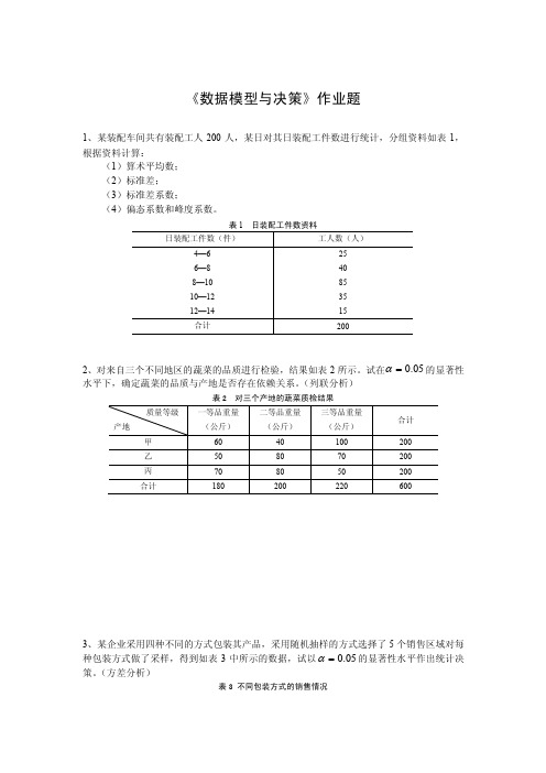
《数据模型与决策》作业题1、某装配车间共有装配工人200人,某日对其日装配工件数进行统计,分组资料如表1,根据资料计算:(1)算术平均数; (2)标准差;(3)标准差系数;(4)偏态系数和峰度系数。
表1 日装配工件数资料日装配工件数(件)工人数(人)4—6 6—8 8—10 10—12 12—14 25 40 85 35 15 合计2002、对来自三个不同地区的蔬菜的品质进行检验,结果如表2所示。
试在05.0=α的显著性水平下,确定蔬菜的品质与产地是否存在依赖关系。
(列联分析)表2 对三个产地的蔬菜质检结果质量等级 产地一等品重量 (公斤)二等品重量 (公斤)三等品重量 (公斤) 合计 甲 60 40 100 200 乙 50 80 70 200 丙 70 80 50 200 合计1802002206003、某企业采用四种不同的方式包装其产品,采用随机抽样的方式选择了5个销售区域对每种包装方式做了采样,得到如表3中所示的数据,试以05.0=α的显著性水平作出统计决策。
(方差分析)表3 不同包装方式的销售情况包装方式 销售区域方式一 方式二 方式三 方式四 1 66 32 46 25 2 45 16 32 15 3 78 66 12 30 4 25 23 45 16 5344650404、已知我国1990年~1999年的货运量y 、工业总产值x 1、农业总产值x 2资料如表4所示:表4 1990年~1999年我国货运量、工业总产值和农业总产值资料年份 货运量(万吨)工业总产值(亿元)农业总产值(亿元)1990 970602 23924 7662.1 1991 985793 26625 8157.0 1992 1045899 34599 9084.7 1993 1115771 48402 10995.5 1994 1180273 70176 15750.5 1995 1234810 91894 20340.9 1996 1296200 99595 22353.7 1997 1278087 113733 23788.4 1998 1267200 119048 24541.9 1999129265012611124519.1要求计算:(1)相关系数(2)二元线性回归方程(3)进行各种统计显著性检验。
数据模型与决策--作业大全详解
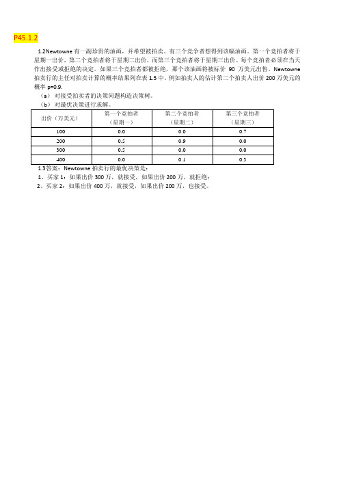
P45.1.21.2N ewtowne有一副珍贵的油画,并希望被拍卖。
有三个竞争者想得到该幅油画。
第一个竞拍者将于星期一出价,第二个竞拍者将于星期二出价,而第三个竞拍者将于星期三出价。
每个竞拍者必须在当天作出接受或拒绝的决定。
如果三个竞拍者都被拒绝,那个该油画将被标价90万美元出售。
Newtowne 拍卖行的主任对拍卖计算的概率结果列在表1.5中。
例如拍卖人的估计第二个拍卖人出价200万美元的概率p=0.9.(a)对接受拍卖者的决策问题构造决策树。
1、买家1:如果出价300万,就接受,如果出价200万,就拒绝;2、买家2:如果出价400万,就接受,如果出价200万,也接受。
接受买家1200 200200接受买家22002002000.50.9接受买家3买家1出价200万买家2出价200万0.7100 21买家3出价100万100100 0220020010100拒绝买家390拒绝买家290900190接受买家30.3400买家3出价400万400400拒绝买家1104000220拒绝买家3909090接受买家24004004000.1接受买家3买家2出价400万0.71001买家3出价100万100100040010100260拒绝买家390拒绝买家290900190接受买家30.3400买家3出价400万40040010400拒绝买家3909090接受买家1300 300300接受买家22002002000.50.9接受买家3买家1出价300万买家2出价200万0.7100 11买家3出价100万100100 0300020010100拒绝买家390拒绝买家290900190接受买家30.3400买家3出价400万400400拒绝买家1104000220拒绝买家3909090接受买家24004004000.1接受买家3买家2出价400万0.71001买家3出价100万100100040010100拒绝买家390拒绝买家290900190接受买家30.3400买家3出价400万40040010400拒绝买家39090902.9在美国有55万人感染HIV病毒。
数据模型与决策(运筹学)课后习题和案例答案(6)

CHAPTER 7NETWORK OPTIMIZATION PROBLEMS Review Questions7.1-1 A supply node is a node where the net amount of flow generated is a fixed positive number.A demand node is a node where the net amount of flow generated is a fixed negativenumber. A transshipment node is a node where the net amount of flow generated is fixed at zero.7.1-2 The maximum amount of flow allowed through an arc is referred to as the capacity of thatarc.7.1-3 The objective is to minimize the total cost of sending the available supply through thenetwork to satisfy the given demand.7.1-4 The feasible solutions property is necessary. It states that a minimum cost flow problemwill have a feasible solution if and only if the sum of the supplies from its supply nodesequals the sum of the demands at its demand nodes.7.1-5 As long as all its supplies and demands have integer values, any minimum cost flowproblem with feasible solutions is guaranteed to have an optimal solution with integervalues for all its flow quantities.7.1-6 Network simplex method.7.1-7 Applications of minimum cost flow problems include operation of a distribution network,solid waste management, operation of a supply network, coordinating product mixes atplants, and cash flow management.7.1-8 Transportation problems, assignment problems, transshipment problems, maximum flowproblems, and shortest path problems are special types of minimum cost flow problems. 7.2-1 One of the company’s most important distribution centers (Los Angeles) urgently needs anincreased flow of shipments from the company.7.2-2 Auto replacement parts are flowing through the network from the company’s main factoryin Europe to its distribution center in LA.7.2-3 The objective is to maximize the flow of replacement parts from the factory to the LAdistribution center.7.3-1 Rather than minimizing the cost of the flow, the objective is to find a flow plan thatmaximizes the amount flowing through the network from the source to the sink.7.3-2 The source is the node at which all flow through the network originates. The sink is thenode at which all flow through the network terminates. At the source, all arcs point awayfrom the node. At the sink, all arcs point into the node.7.3-3 The amount is measured by either the amount leaving the source or the amount entering thesink.7.3-4 1. Whereas supply nodes have fixed supplies and demand nodes have fixed demands, thesource and sink do not.2. Whereas the number of supply nodes and the number of demand nodes in a minimumcost flow problem may be more than one, there can be only one source and only onesink in a standard maximum flow problem.7.3-5 Applications of maximum flow problems include maximizing the flow through adistribution network, maximizing the flow through a supply network, maximizing the flow of oil through a system of pipelines, maximizing the flow of water through a system ofaqueducts, and maximizing the flow of vehicles through a transportation network.7.4-1 The origin is the fire station and the destination is the farm community.7.4-2 Flow can go in either direction between the nodes connected by links as opposed to onlyone direction with an arc.7.4-3 The origin now is the one supply node, with a supply of one. The destination now is theone demand node, with a demand of one.7.4-4 The length of a link can measure distance, cost, or time.7.4-5 Sarah wants to minimize her total cost of purchasing, operating, and maintaining the carsover her four years of college.7.4-6 When “real travel” through a network can end at more that one node, a dummy destinationneeds to be added so that the network will have just a single destination.7.4-7 Quick’s management must consider trade-offs between time and cost in making its finaldecision.7.5-1 The nodes are given, but the links need to be designed.7.5-2 A state-of-the-art fiber-optic network is being designed.7.5-3 A tree is a network that does not have any paths that begin and end at the same nodewithout backtracking. A spanning tree is a tree that provides a path between every pair of nodes. A minimum spanning tree is the spanning tree that minimizes total cost.7.5-4 The number of links in a spanning tree always is one less than the number of nodes.Furthermore, each node is directly connected by a single link to at least one other node. 7.5-5 To design a network so that there is a path between every pair of nodes at the minimumpossible cost.7.5-6 No, it is not a special type of a minimum cost flow problem.7.5-7 A greedy algorithm will solve a minimum spanning tree problem.17.5-8 Applications of minimum spanning tree problems include design of telecommunicationnetworks, design of a lightly used transportation network, design of a network of high- voltage power lines, design of a network of wiring on electrical equipment, and design of a network of pipelines.Problems7.1a)b)c)1[40] 6 S17 4[-30] D1 [-40] D2 [60] 5 8S2 6[-30] D37.2a)supply nodestransshipment nodesdemand nodesb)[200] P1560 [150]425 [125][0] W1505[150]490 [100]470 [100][-150]RO1[-200]RO2P2 [300]c)510 [175]600 [200][0] W2390 [125]410[150] 440[75]RO3[-150]7.3a)supply nodestransshipment nodesdemand nodesV1W1F1V2V3W2 F21P1W1RO1RO2P2W2RO3[-50] SE3000[20][0]BN5700[40][0]HA[50]BE 4000 6300[40][30] [0][0]NY2000[60]2400[20]3400[10] 4200[80][0]5900[60]5400[40]6800[50]RO[0]BO[0]2500[70]2900[50]b)c)7.4a)LA 3100 NO 6100 LI 3200 ST[-130] [70] [30] [40] [130]1[70]11b)c) The total shipping cost is $2,187,000.7.5a)[0][0] 5900RONY[60] 5400[0] 2900 [50]4200 [80][0] [40] 6800 [50]BO[0] 2500LA 3100 NO 6100 LI 3200 ST [-130][70][30] [40][130]b)c)SEBNHABERONYNY(80) [80] (50) [60](30)[40] ROBO (40)(50) [50] (70)[70]11d)e)f) $1,618,000 + $583,000 = $2,201,000 which is higher than the total in Problem 7.5 ($2,187,000). 7.6LA(70) NO[50](30)LI (30) ST[70][30] [40]There are only two arcs into LA, with a combined capacity of 150 (80 + 70). Because ofthis bottleneck, it is not possible to ship any more than 150 from ST to LA. Since 150 actually are being shipped in this solution, it must be optimal. 7.7[-50] SE3000 [20] [0] BN 5700 [40][0] HA[50] BE4000 6300[40][0] NY2000 [60] 2400 [20][30] [0]5900RO [60]17.8 a) SourcesTransshipment Nodes Sinkb)7.9 a)AKR1[75]A [60]R2[65] [40][50][60] [45]D [120] [70]B[55]E[190]T [45][80] [70][70]R3CF[130][90]SE PT KC SL ATCHTXNOMES S F F CAb)Oil Fields Refineries Distribution CentersTXNOPTCACHATAKSEKCME c)SLSFTX[11][7] NO[5][9] PT[8] [2][5] CA [4] [7] [8] [7] [4] [6][8] CH [7][5][9] [4] ATAK [3][6][6][12] SE KC[8][9][4][8] [7] [12] [11]MESL [9]SF[15][7]d)3Shortest path: Fire Station – C – E – F – Farming Community 7.11 a)A70D40 60O60 5010 B 20 C5540 10 T50E801c)Shortest route: Origin – A – B – D – Destinationd)Yese)Yes7.12a)31,00018,000 21,00001238,000 10,000 12,000b)17.13a) Times play the role of distances.B 2 2 G5ACE 1 31 1b)7.14D F1. C---D: Cost = 14.E---G: Cost = 5E---F: Cost = 1 *choose arbitrarilyD---A: Cost = 4 2.E---G: Cost = 5 E---B: Cost = 7 E---B: Cost = 7 F---G: Cost = 7 E---C: Cost = 4 C---A: Cost = 5F---G: Cost = 7C---B: Cost = 2 *lowestF---C: Cost = 3 *lowest5.E---G: Cost = 5 F---D: Cost = 4 D---A: Cost = 43. E---G: Cost = 5 B---A: Cost = 2 *lowestE---B: Cost = 7 F---G: Cost = 7 F---G: Cost = 7 C---A: Cost = 5F---D: Cost = 46.E---G: Cost = 5 *lowestC---D: Cost = 1 *lowestF---G: Cost = 7C---A: Cost = 5C---B: Cost = 2Total = $14 million7.151. B---C: Cost = 1 *lowest 4. B---E: Cost = 72. B---A: Cost = 4 C---F: Cost = 4 *lowestB---E: Cost = 7 C---E: Cost = 5C---A: Cost = 6 D---F: Cost = 5C---D: Cost = 2 *lowest 5. B---E: Cost = 7C---F: Cost = 4 C---E: Cost = 5C---E: Cost = 5 F---E: Cost = 1 *lowest3. B---A: Cost = 4 *lowest F---G: Cost = 8B---E: Cost = 7 6. E---G: Cost = 6 *lowestC---A: Cost = 6 F---G: Cost = 8C---F: Cost = 4C---E: Cost = 5D---A: Cost = 5 Total = $18,000D---F: Cost = 57.16B 34 2E HA D 2 G I K3C F 12J34B41E6A C41G2 FD1. F---G: Cost = 1 *lowest 6. D---A: Cost = 62. F---C: Cost = 6 D---B: Cost = 5F---D: Cost = 5 D---C: Cost = 4F---I: Cost = 2 *lowest E---B: Cost = 3 *lowestF---J: Cost = 5 F---C: Cost = 6G---D: Cost = 2 F---J: Cost = 5G---E: Cost = 2 H---K: Cost = 7G---H: Cost = 2 I---K: Cost = 8G---I: Cost = 5 I---J: Cost = 33. F---C: Cost = 6 7. B---A: Cost = 4F---D: Cost = 5 D---A: Cost = 6F---J: Cost = 5 D---C: Cost = 4G---D: Cost = 2 *lowest F---C: Cost = 6G---E: Cost = 2 F---J: Cost = 5G---H: Cost = 2 H---K: Cost = 7I---H: Cost = 2 I---K: Cost = 8I---K: Cost = 8 I---J: Cost = 3 *lowestI---J: Cost = 3 8. B---A: Cost = 4 *lowest4. D---A: Cost = 6 D---A: Cost = 6D---B: Cost = 5 D---C: Cost = 4D---E: Cost = 2 *lowest F---C: Cost = 6D---C: Cost = 4 H---K: Cost = 7F---C: Cost = 6 I---K: Cost = 8F---J: Cost = 5 J---K: Cost = 4G---E: Cost = 2 9. A---C: Cost = 3 *lowestG---H: Cost = 2 D---C: Cost = 4I---H: Cost = 2 F---C: Cost = 6I---K: Cost = 8 H---K: Cost = 7I---J: Cost = 3 I---K: Cost = 85. D---A: Cost = 6 J---K: Cost = 4D---B: Cost = 5 10. H---K: Cost = 7D---C: Cost = 4 I---K: Cost = 8E---B: Cost = 3 J---K: Cost = 4 *lowestE---H: Cost = 4F---C: Cost = 6F---J: Cost = 5G---H: Cost = 2 *lowest Total = $26 millionI---H: Cost = 2I---K: Cost = 8I---J: Cost = 37.17a) The company wants a path between each pair of nodes (groves) that minimizes cost(length of road).b)7---8 : Distance = 0.57---6 : Distance = 0.66---5 : Distance = 0.95---1 : Distance = 0.75---4 : Distance = 0.78---3 : Distance = 1.03---2 : Distance = 0.9Total = 5.3 miles7.18a) The bank wants a path between each pair of nodes (offices) that minimizes cost(distance).b) B1---B5 : Distance = 50B5---B3 : Distance = 80B1---B2 : Distance = 100B2---M : Distance = 70B2---B4 : Distance = 120Total = 420 milesHamburgBostonRotterdamSt. PetersburgNapoliMoscowA IRFIELD SLondonJacksonvilleBerlin RostovIstanbulCases7.1a) The network showing the different routes troops and supplies may follow to reach the Russian Federation appears below.PORTSb)The President is only concerned about how to most quickly move troops and suppliesfrom the United States to the three strategic Russian cities. Obviously, the best way to achieve this goal is to find the fastest connection between the US and the three cities.We therefore need to find the shortest path between the US cities and each of the three Russian cities.The President only cares about the time it takes to get the troops and supplies to Russia.It does not matter how great a distance the troops and supplies cover. Therefore we define the arc length between two nodes in the network to be the time it takes to travel between the respective cities. For example, the distance between Boston and London equals 6,200 km. The mode of transportation between the cities is a Starlifter traveling at a speed of 400 miles per hour * 1.609 km per mile = 643.6 km per hour. The time is takes to bring troops and supplies from Boston to London equals 6,200 km / 643.6 km per hour = 9.6333 hours. Using this approach we can compute the time of travel along all arcs in the network.By simple inspection and common sense it is apparent that the fastest transportation involves using only airplanes. We therefore can restrict ourselves to only those arcs in the network where the mode of transportation is air travel. We can omit the three port cities and all arcs entering and leaving these nodes.The following six spreadsheets find the shortest path between each US city (Boston and Jacksonville) and each Russian city (St. Petersburg, Moscow, and Rostov).The spreadsheets contain the following formulas:Comparing all six solutions we see that the shortest path from the US to Saint Petersburg is Boston → London → Saint Petersburg with a total travel time of 12.71 hours. The shortest path from the US to Moscow is Boston → London → Moscow with a total travel time of 13.21 hours. The shortest path from the US to Rostov is Boston →Berlin → Rostov with a total travel time of 13.95 hours. The following network diagram highlights these shortest paths.-1c)The President must satisfy each Russian city’s military requirements at minimum cost.Therefore, this problem can be solved as a minimum-cost network flow problem. The two nodes representing US cities are supply nodes with a supply of 500 each (wemeasure all weights in 1000 tons). The three nodes representing Saint Petersburg, Moscow, and Rostov are demand nodes with demands of –320, -440, and –240,respectively. All nodes representing European airfields and ports are transshipment nodes. We measure the flow along the arcs in 1000 tons. For some arcs, capacityconstraints are given. All arcs from the European ports into Saint Petersburg have zero capacity. All truck routes from the European ports into Rostov have a transportation limit of 2,500*16 = 40,000 tons. Since we measure the arc flows in 1000 tons, the corresponding arc capacities equal 40. An analogous computation yields arc capacities of 30 for both the arcs connecting the nodes London and Berlin to Rostov. For all other nodes we determine natural arc capacities based on the supplies and demands at the nodes. We define the unit costs along the arcs in the network in $1000 per 1000 tons (or, equivalently, $/ton). For example, the cost of transporting 1 ton of material from Boston to Hamburg equals $30,000 / 240 = $125, so the costs of transporting 1000 tons from Boston to Hamburg equals $125,000.The objective is to satisfy all demands in the network at minimum cost. The following spreadsheet shows the entire linear programming model.HamburgBoston Rotterdam St.Petersburg+500-320Napoli Moscow A IRF IELDSLondon -440Jacksonville Berlin Rostov+500-240Istanbul The total cost of the operation equals $412.867 million. The entire supply for SaintPetersburg is supplied from Jacksonville via London. The entire supply for Moscow is supplied from Boston via Hamburg. Of the 240 (= 240,000 tons) demanded by Rostov, 60 are shipped from Boston via Istanbul, 150 are shipped from Jacksonville viaIstanbul, and 30 are shipped from Jacksonville via London. The paths used to shipsupplies to Saint Petersburg, Moscow, and Rostov are highlighted on the followingnetwork diagram.PORTSd)Now the President wants to maximize the amount of cargo transported from the US tothe Russian cities. In other words, the President wants to maximize the flow from the two US cities to the three Russian cities. All the nodes representing the European ports and airfields are once again transshipment nodes. The flow along an arc is againmeasured in thousands of tons. The new restrictions can be transformed into arccapacities using the same approach that was used in part (c). The objective is now to maximize the combined flow into the three Russian cities.The linear programming spreadsheet model describing the maximum flow problem appears as follows.The spreadsheet shows all the amounts that are shipped between the various cities. The total supply for Saint Petersburg, Moscow, and Rostov equals 225,000 tons, 104,800 tons, and 192,400 tons, respectively. The following network diagram highlights the paths used to ship supplies between the US and the Russian Federation.PORTSHamburgBoston Rotterdam St.Petersburg+282.2 -225NapoliMoscowAIRFIELDS-104.8LondonJacksonvilleBerlin Rostov +240 -192.4Istanbule)The creation of the new communications network is a minimum spanning tree problem.As usual, a greedy algorithm solves this type of problem.Arcs are added to the network in the following order (one of several optimal solutions):Rostov - Orenburg 120Ufa - Orenburg 75Saratov - Orenburg 95Saratov - Samara 100Samara - Kazan 95Ufa – Yekaterinburg 125Perm – Yekaterinburg 857.2a) There are three supply nodes – the Yen node, the Rupiah node, and the Ringgit node.There is one demand node – the US$ node. Below, we draw the network originatingfrom only the Yen supply node to illustrate the overall design of the network. In thisnetwork, we exclude both the Rupiah and Ringgit nodes for simplicity.b)Since all transaction limits are given in the equivalent of $1000 we define the flowvariables as the amount in thousands of dollars that Jake converts from one currencyinto another one. His total holdings in Yen, Rupiah, and Ringgit are equivalent to $9.6million, $1.68 million, and $5.6 million, respectively (as calculated in cells I16:K18 inthe spreadsheet). So, the supplies at the supply nodes Yen, Rupiah, and Ringgit are -$9.6 million, -$1.68 million, and -$5.6 million, respectively. The demand at the onlydemand node US$ equals $16.88 million (the sum of the outflows from the sourcenodes). The transaction limits are capacity constraints for all arcs leaving from thenodes Yen, Rupiah, and Ringgit. The unit cost for every arc is given by the transactioncost for the currency conversion.Jake should convert the equivalent of $2 million from Yen to each US$, Can$, Euro, and Pound. He should convert $1.6 million from Yen to Peso. Moreover, he should convert the equivalent of $200,000 from Rupiah to each US$, Can$, and Peso, $1 million from Rupiah to Euro, and $80,000 from Rupiah to Pound. Furthermore, Jake should convert the equivalent of $1.1 million from Ringgit to US$, $2.5 million from Ringgit to Euro, and $1 million from Ringgit to each Pound and Peso. Finally, he should convert all the money he converted into Can$, Euro, Pound, and Peso directly into US$. Specifically, he needs to convert into US$ the equivalent of $2.2 million, $5.5 million, $3.08 million, and $2.8 million Can$, Euro, Pound, and Peso, respectively. Assuming Jake pays for the total transaction costs of $83,380 directly from his American bank accounts he will have $16,880,000 dollars to invest in the US.c)We eliminate all capacity restrictions on the arcs.Jake should convert the entire holdings in Japan from Yen into Pounds and then into US$, the entire holdings in Indonesia from Rupiah into Can$ and then into US$, and the entire holdings in Malaysia from Ringgit into Euro and then into US$. Without the capacity limits the transaction costs are reduced to $67,480.d)We multiply all unit cost for Rupiah by 6.The optimal routing for the money doesn't change, but the total transaction costs are now increased to $92,680.e)In the described crisis situation the currency exchange rates might change every minute.Jake should carefully check the exchange rates again when he performs thetransactions.The European economies might be more insulated from the Asian financial collapse than the US economy. To impress his boss Jake might want to explore other investment opportunities in safer European economies that provide higher rates of return than US bonds.。
数据模型与决策课程学习大作业.doc

数据模型与决策课程大作业以我国汽油消费量为因变量,乘用车销量、城镇化率和90#汽油吨价与城镇居民人均可支配收入的比值为自变量时行回归(数据为年度时间序列数据)。
试根据得到部分输出结果,回答下列问题:1)“模型汇总表”中的R方和标准估计的误差是多少?2)写出此回归分析所对应的方程;3)将三个自变量对汽油消费量的影响程度进行说明;4)对回归分析结果进行分析和评价,指出其中存在的问题。
1)“模型汇总表”中的R方和标准估计的误差是多少?答案:R方为0.993^2=0.986 ;标准估计的误差为120910.147^(0.5)=347.722)写出此回归分析所对应的方程;答案:假设汽油消费量为Y,乘用车销量为a,城镇化率为b,90#汽油吨价/城镇居民人均可支配收入为c,则回归方程为:Y=240.534+0.00s027a+8649.895b-198.692c3)将三个自变量对汽油消费量的影响程度进行说明;乘用车销量对汽油消费量相关系数只有0.00027,数值太小,几乎没有影响,但是城镇化率对汽油消费量相关系数是8649.895,具有明显正相关,当城镇化率每提高1,汽油消费量增加8649.895。
乘用90#汽油吨价/城镇居民人均可支配收入相关系数为-198.692,呈明显负相关,即乘用90#汽油吨价/城镇居民人均可支配收入每增加1个单位,汽油消费量降低198.692个单位。
a, b, c三个自变量的sig 值为0.000、0.000、0.009,在显著性水平0.01情形下,乘用车消费量对汽油消费量的影响显著为正。
(4)对回归分析结果进行分析和评价,指出其中存在的问题。
在学习完本课程之后,我们可以统计方法为特征的不确定性决策、以运筹方法为特征的策略的基本原理和一般方法为基础,结合抽样、参数估计、假设分析、回归分析等知识对我国汽油消费量影响因素进行了模拟回归,并运用软件计算出回归结果,故根据回归结果,对具体回归方程,回归准确性,自变量影响展开分析。
数据模型与决策课
数据模型与决策课程大作业数据模型与决策课程大作业以我国汽油消费量为因变量,乘用车销量、城镇化率和90#汽油吨价与城镇居民人均可支配收入的比值为自变量时行回归(数据为年度时间序列数据)。
试根据得到部分输出结果,回答下列问题:1)“模型汇总表”中的R方和标准估计的误差是多少?2)写出此回归分析所对应的方程;3)将三个自变量对汽油消费量的影响程度进行说明;4)对回归分析结果进行分析和评价,指出其中存在的问题。
1)“模型汇总表”中的R方和标准估计的误差是多少?答案:R方为0.993^2=0.986 ;标准估计的误差为120910.147^(0.5)=347.722)写出此回归分析所对应的方程;答案:假设汽油消费量为Y,乘用车销量为a,城镇化率为b,90#汽油吨价/城镇居民人均可支配收入为c,则回归方程为:Y=240.534+0.00s027a+8649.895b-198.692c3)将三个自变量对汽油消费量的影响程度进行说明;乘用车销量对汽油消费量相关系数只有0.00027,数值太小,几乎没有影响,但是城镇化率对汽油消费量相关系数是8649.895,具有明显正相关,当城镇化率每提高1,汽油消费量增加8649.895。
乘用90#汽油吨价/城镇居民人均可支配收入相关系数为-198.692,呈明显负相关,即乘用90#汽油吨价/城镇居民人均可支配收入每增加1个单位,汽油消费量降低198.692个单位。
a, b, c三个自变量的sig 值为0.000、0.000、0.009,在显著性水平0.01情形下,乘用车消费量对汽油消费量的影响显著为正。
(4)对回归分析结果进行分析和评价,指出其中存在的问题。
在学习完本课程之后,我们可以统计方法为特征的不确定性决策、以运筹方法为特征的策略的基本原理和一般方法为基础,结合抽样、参数估计、假设分析、回归分析等知识对我国汽油消费量影响因素进行了模拟回归,并运用软件计算出回归结果,故根据回归结果,对具体回归方程,回归准确性,自变量影响展开分析。
《数据模型与决策》练习题及答案
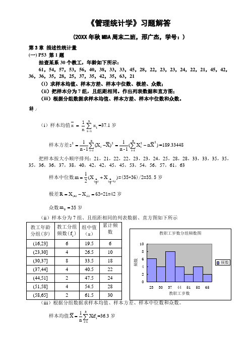
《管理统计学》习题解答(20XX 年秋MBA 周末二班,邢广杰,学号:)第3章 描述性统计量 (一) P53 第1题抽查某系30个教工,年龄如下所示:61,54,57,53,56,40,38,33,33,45,28,22,23,23,24,22,21,45,42,36,36,35,28,25,37,35,42,35,63,21(i )求样本均值、样本方差、样本中位数、极差、众数;(ii )把样本分为7组,且组距相同。
作出列表数据和直方图; (iii )根据分组数据求样本均值、样本方差、样本中位数和众数。
解:(i )样本均值∑==n1i ixn1x =37.1岁样本方差)X n X (1-n 1)X (X 1-n 1s 2n 1i 2i2n 1i i 2-=-=∑∑===189.33448 把样本按大小顺序排列:21,21,22,22,23,23,24,25,28,28,33,33,35,35,35,36,36,37,38,40,42,42,45,45,53,54,56,57,61,63样本中位数)X X (21m 1)2n ()2n (++==(35+36)/2=35.5岁极差=-=1)()n (X X R 63-21=42岁 众数=0m 35岁(ii )样本分为7组、且组距相同的列表数据、直方图如下所示样本均值i k1i f Xi n 1X ∑===36.3岁样本方差)X n f X (1-n 1f )X (X 1-n 1s 2k 1i i 2i i2k 1i i 2-=-=∑∑===174.3724 样本中位数810230730f F 2n i I m -+=-+==34.375岁 众数=--⨯-+=---+=+448248730f f 2f f f iI m 1m 1-m m 1-m m 033.5岁(二)P53 第2题某单位统计了不同级别的员工的月工资水平资料如下:解:样本均值i k1i f Xi n 1X ∑===1566.667元样本标准差)X n f X (1-n 1f )X (X 1-n 1s 2k 1i i2i i 2k 1i i -=-=∑∑===398.1751元 样本中位数在累计74人的那一组,m=1500元; 众数1500m 0=元。
- 1、下载文档前请自行甄别文档内容的完整性,平台不提供额外的编辑、内容补充、找答案等附加服务。
- 2、"仅部分预览"的文档,不可在线预览部分如存在完整性等问题,可反馈申请退款(可完整预览的文档不适用该条件!)。
- 3、如文档侵犯您的权益,请联系客服反馈,我们会尽快为您处理(人工客服工作时间:9:00-18:30)。
特赛格案例的继续研究
背景信息:
教材上描述了特赛格想要在三个地址中间选择一个来建造新炼油厂,通过对原油和成品油运输成本的分析,最终选定了圣路易斯作为新炼油厂。
但是为了准备面对可能的市场需求的增长,管理者希望扩大新炼油厂的生产能力到1.5亿桶,并且需要计算在1.5亿桶的情况下,去运送3.6亿桶油选择圣路易斯是不是仍能够保证最优的运输计划。
(假设运营成本不变)接下来从下面几个步骤来分析问题:
a. 如果新炼油厂的生产能力增加到1.5亿桶,比较与之前生产1.2亿桶的运输成本差别
图1. 生产1.2亿桶的圣路易斯炼油厂的原油年运输成本(运输3.6亿桶)
图2.生产1.5亿桶的圣路易斯炼油厂的原油年运输成本(运输3.6亿桶)
从上面最优解计算可以看出,扩大产能后,圣路易斯的原油年运输成本从9.6减少到9.4亿美元
b. 假设a中求出的计划将被采用,即原油到炼油厂的运输如表2所示,在计算产成品油到配送中心的最优运输方案
图3. 生产1.2亿桶的圣路易斯炼油厂的成品油年运输成本(运输3.6亿桶)
图4. 生产1.5亿桶的圣路易斯炼油厂的成品油年运输成本(运输3.6亿桶)
从上面最优解计算可以看出,扩大产能后,圣路易斯的成品油年运输成本从14.3减少到13.9亿美元
因此,扩大产能后,原油和成品油总的运输成本从23.9亿美元降到23.3亿美元
c&d. 运输成品油的成本大于运输原油的成本,所以考虑最小化运送成品油运输成本为基础,建立电子表格模型并求解如下
图5.先考虑运输成品油
这样规划以后可以看出,圣路易斯的成品油年运输成本进一步从13.9亿降到13.55亿美元。
并且以此为基础再计算原油运输成本的最优解如下
图6.再考虑运输原油
此时,圣路易斯的原油年运输成本增加到9.8亿美元,而原油和成品油总的运输成本是 23.35亿美元.因此此方案不如b的方案好。
以上各种方案比较见下表
e. 以上的分析都是分布优化决定,因为每次都只能使其中一部分得到最优化,所以现在应该进一步考虑。
同时考虑将3.6亿桶原油从产地运往炼油厂,再运往配送中心的运输计划。
目标使总的运输成本最小。
重新建立电子表格模型如下图所示,并求得最优解。
图7 按照整体优化的思路寻找最优解-圣路易斯
由此可知,圣路易斯的原油年运输成本为9.5亿美元,成品油年运输成本为13.7亿美元,总运输成本为23.20亿美元。
将此结果与前面计算的bcd结果比较,发现此结果最优。
f.如果选择洛杉矶为新炼油厂的地址,做电子表格模型并求最优解,结果如下
图8 按照整体优化的思路寻找最优解-洛杉矶
如果选择加尔维斯顿为新炼油厂的地址,做电子表格模型并求最优解,结果如下
图9 按照整体优化的思路寻找最优解-加尔维斯顿
考虑书中表6.19的运营成本,对三个地方进行财务比较
g.给管理层的建议
基于教材中特赛格公司的选址问题,最终公司决定选择圣路易斯作为新炼油厂。
但是,为了准备面对可能的市场需求的增长,管理者希望过大炼油厂的生产能力到1.5亿桶。
经过对以上三个建造新炼油厂备选地点的财务分析。
表4显示了对于三个可能建造新炼油厂的每一个备选地每年所有的主要可变成本。
表2以前的分析表明了,扩大产能,虽然目前还用不上,但是有助于降低总的运输费用。
并且应该将原油和成品油运输的情况放在一起考虑求得的运输方案能带来最小的运输成本。
同时将扩大产能的想法在另外两个备选地址进行验证,发现圣路易斯仍然是最优选择。
因此,应该建议管理层选择在圣路易斯建造新的炼油厂,并且扩大产能到1.5亿桶,使用原油和成品油运输的情况放在一起考虑求得的运输方案,最终可达到每年总变动成本最小,即28.5亿美元。