ARIMA模型在SPSS中的推算过程
以数学建模竞赛为例基于spss建立arima模型

20201/295徐燕1981要/数理统计学专业副教授/博士/广州民航职业技术学院人文社科学院/南方医科大学访问学者/从事统计学方法和应用研究工作(广州510403)以数学建模竞赛为例基于SPSS 建立ARIMA 模型Combined with learning pass and BOPPPS model to improve the teaching effect of electrical science徐燕基金项目:2019年高等学校中青年教师国内访问学者项目资助。
摘要SPSS 软件是当前应用最广泛的统计软件之一,其菜单化操作模式能够让使用者快速入门,SPSS 软件中时间序列模块能够实现模型的自动化筛选,参数估计和模型检验,是非统计学专业人员进行数据分析的有力工具。
是本文以2019年全国大学生数学建模竞赛D 题为例,以SPSS23软件为工具,对数据进行时间序列分析,建立ARIMA 模型。
关键词数学建模;SPSS;时间序列;ARIMA 模型中图分类号:R058文献标识码:ADOI :10.19694/ki.issn2095-2457.2020.01.160引言SPSS 软件是当前世界上应用最广泛的统计软件之一,菜单化操作、图表化输出的特点特别受到非统计学专业人员的欢迎。
使用SPSS 软件,我们几乎可以完全自动的自变量的预变换、筛选、模型优化、检验等工作。
SPSS 软件中的预测模块,纳入了常用的时间序列分析模型,如ARIMA 模型,包括自动的模型选择、参数估计和模型检验等功能,实现了简单操作即可得到可靠的时间序列模型,其功能得到了使用者的肯定。
近年来,全国大学生数学建模竞赛频频出现大数据统计建模试题,作为非统计学专业的大学生,对于复杂的数据统计分析方法和工具接触并不很多,如何让这些学生快速入门和掌握一门有利的数据分析软件工具、完成数据分析和建模等任务就是我们近几年来数学建模培训教学研究的重点。
以数学建模竞赛为例基于SPSS建立ARIMA模型
以数学建模竞赛为例基于SPSS建立ARIMA模型一、引言数学建模竞赛是在各种学科领域中,通过数学方法解决实际问题的一种竞赛形式。
参加数学建模竞赛需要队员具备一定的数学建模能力,包括数学建模的理论知识、数学工具的使用和数学模型的构建能力。
在数学建模竞赛中,队员需要根据给定的问题和数据,使用数学方法建立合适的数学模型,并进行模型的求解和分析。
数学建模竞赛中的数学建模和数据分析方法对于队员来说是至关重要的。
在本文中,我们将以数学建模竞赛的一个实际问题为例,演示如何利用SPSS软件建立ARIMA模型对相关数据进行预测和分析。
我们将首先介绍ARIMA模型的基本原理和建模流程,然后利用SPSS软件对给定的数据进行ARIMA模型的建立和检验,最后对模型的效果进行评价并给出相关建议。
二、ARIMA模型的基本原理ARIMA模型是时间序列分析中常用的一种模型,用于对时间序列数据进行预测和分析。
ARIMA模型包括自回归(AR)、差分(I)和移动平均(MA)三部分,分别表示时间序列数据中的自相关、季节性趋势和误差项。
ARIMA模型的建立包括模型的识别、参数的估计和模型的检验三个步骤。
1. 模型的识别:首先需要对时间序列数据进行平稳性和自相关性检验,确定ARIMA模型的参数p、d、q。
p表示自回归的阶数,d表示差分的阶数,q表示移动平均的阶数。
2. 参数的估计:利用最大似然估计等方法,对ARIMA模型中的参数进行估计,得到模型的估计系数。
3. 模型的检验:对估计的ARIMA模型进行残差分析和预测检验,对模型的拟合效果进行评价,并进行模型的调整和优化。
三、SPSS建立ARIMA模型的步骤在SPSS软件中,利用时间序列建模功能可以方便地进行ARIMA模型的建立和分析。
下面我们以一个实际的数据为例,演示在SPSS中建立ARIMA模型的具体步骤。
1. 数据导入:首先在SPSS中导入要分析的时间序列数据,可以是Excel表格或者文本文件格式。
spss时间序列模型
《统计软件实验报告》SPSS软件的上机实践应用时间序列分析数学与统计学学院一、实验内容:时间序列是指一个依时间顺序做成的观察资料的集合。
时间序列分析过程中最常用的方法是:指数平滑、自回归、综合移动平均及季节分解。
本次实验研究就业理论中的就业人口总量问题。
但人口经济的理论和实践表明,就业总量往往受到许多因素的制约,这些因素之间有着错综复杂的联系,因此,运用结构性的因果模型分析和预测就业总量往往是比较困难的。
时间序列分析中的自回归求积分移动平均法(ARIMA)则是一个较好的选择。
对于时间序列的短期预测来说,随机时序ARIMA是一种精度较高的模型。
我们已XX省历年(1969-2005)从业人员人数为数据基础建立一个就业总量的预测时间序列模型,通过spss建立模型并用此模型来预测就业总量的未来发展趋势。
二、实验目的:1.准确理解时间序列分析的方法原理2.学会实用SPSS建立时间序列变量3.学会使用SPSS绘制时间序列图以反应时间序列的直观特征。
4.掌握时间序列模型的平稳化方法。
5.掌握时间序列模型的定阶方法。
6.学会使用SPSS建立时间序列模型与短期预测。
7.培养运用时间序列分析方法解决身边实际问题的能力。
三、实验分析:总体分析:先对数据进行必要的预处理和观察,直到它变成稳态后再用SPSS对数据进行分析。
数据的预处理阶段,将它分为三个步骤:首先,对有缺失值的数据进行修补,其次将数据资料定义为相应的时间序列,最后对时间序列数据的平稳性进行计算观察。
数据分析和建模阶段:根据时间序列的特征和分析的要求,选择恰当的模型进行数据建模和分析。
四、实验步骤:SPSS的数据准备包括数据文件的建立、时间定义和数据期间的指定。
SPSS的时间定义功能用来将数据编辑窗口中的一个或多个变量指定为时间序列变量,并给它们赋予相应的时间标志,具体操作步骤是:1.选择菜单:Date→Define Dates,出现窗口:单击【ok(确认)】按钮,此时完成时间的定义,SPSS将在当前数据编辑窗口中自动生成标志时间的变量。
ARIMA预测原理以及SAS实现代码
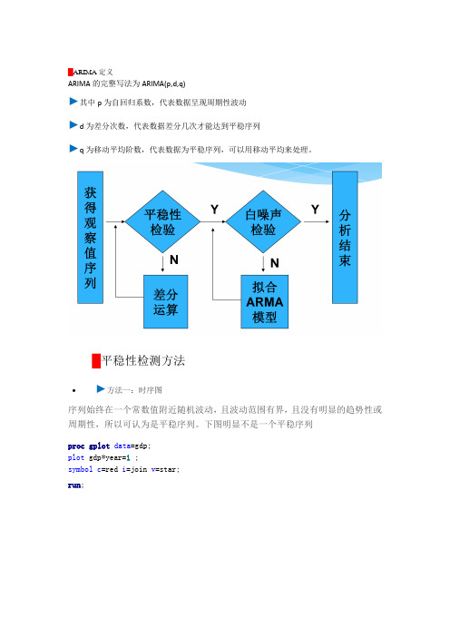
█ARIMA定义ARIMA的完整写法为ARIMA(p,d,q)►其中p为自回归系数,代表数据呈现周期性波动►d为差分次数,代表数据差分几次才能达到平稳序列►q为移动平均阶数,代表数据为平稳序列,可以用移动平均来处理。
█平稳性检测方法•►方法一:时序图序列始终在一个常数值附近随机波动,且波动范围有界,且没有明显的趋势性或周期性,所以可认为是平稳序列。
下图明显不是一个平稳序列proc gplot data=gdp;plot gdp*year=1 ;symbol c=red i=join v=star;run;•►方法二:自相关图自相关系数会很快衰减向0,所以可认为是平稳序列。
proc arima data= gdp;identify var=gdp stationarity =(adf=3) nlag=12;run;•►ADF单位根检验(精确判断)三个检验中只要有一个Pr<Rho小于0.05即可认定为平稳序列,主要是stationarity=(adf=3) 起作用proc arima data= gdp;identify var=gdp stationarity =(adf=3) nlag=12; run;█白噪声检验Pr>卡方<0.05即可认定为通过白噪声检验。
proc arima data= gdp;identify var=gdp stationarity =(adf=3) nlag=12; run;█非平稳序列转换为平稳序列方法一:将数据取对数。
方法二:对数据取差分dif函数data gdp_log;set gdp;loggdp=log(gdp);cfloggdp=dif(loggdp);run;/**对数数据散点图**/proc gplot;plot loggdp*year=1 ;symbol c=black i=join v=star; run;/* 一阶差分对数数据散点图*/ proc gplot;plot cfloggdp*year=1;symbol c=green v=dot i=join;run;从上图中可以看出,一阶差分后序列已经变成平稳的了,因此,数列需要做一阶差分█转换完毕后再验证下面代码中的(1)就代表1阶差分,adf=3则代表平稳性检验0-3,/* 一阶差分对数数据的自相关图、偏自相关图、纯随机性检验、单位根检验 */ proc arima data=gdp_log;identify var=loggdp(1) stationarity =(adf=3) nlag=12;run;用Q LB统计量作的 2检验结果表明:对数差分后的GDP序列的Q LB统计量的P值为0.0045(<0.05),故序列为非白噪声序列。
ARIMA模型

ARIMA模型1.理论ARIMA(自回归综合移动平均):是时间系列分析中最常见的模型,又称Box-Jenkins模型或带差分的自回归移动平均模型。
时间系列的模型确定:时间系列必做步骤:定义日期:点击数据、定义日期(根据数据的时间记录方式,后进行对应的方式定义并填入初始时间):若存在数据缺失:可以采用,该列数据的平均值进行填补或者采用临近的均值:(点击转换、替换缺失值),且需要时间顺序的按一定的顺序进行排序的数据才能进行时间序列的分析。
A.模型初步分析:首先通过分析看数据的模型图情况:(点击分析、时间序列分析、系列图(时间变量需要放入定义后的时间变量))平稳性:时间系列数据可以看作随机过程的一个样本,且根据1.:均值不随时间的变化;2.方差不随时间变化;3.自相关关系只与时间间隔有关而以所处的具体时刻无关。
通常情况下数据在一定的范围内(M±2*SD)波动的话属于平稳,并且如果数据有特别的向下或向上的趋势表明不属于平稳。
B.模型识别与定阶:自相关(ACF)和偏相关操作:(点击分析、时间序列、自相关):自相关系数(如果系数迅速减少的表明属于平稳,系数慢慢的减少说明属于非平稳的),ACF图也可以看出。
判断是否平稳后需要进行差分(平稳化的手段:一般差分、季节性差分)处理:(点击分析、时间系列、自相关(定义好差分介数)):ARIMA模型(p (ACF图:从第几个后进入(2*SD)里表明为几介后),d(差分:做几介差分平稳就填入几),q(PCF图:从第几个后进入(2*SD)里表明为几介后)),拖尾:按指数衰减(呈现正弦波形式),截尾:某一步后为零(迅速降为零)。
平稳化处理后,若偏自相关函数是截尾的,而自相关函数是拖尾的,则建立AR模型;若自相关函数是拖尾的,而偏自相关函数是截尾的,则建立MA模型;若偏自相关函数和自相关函数均是拖尾的,则序列适合ARMA模型。
C.模型估计参数:对识别阶段所给初步模型的参数进行估计及假设检验,并对模型的残差序列做诊断分析,以判断模型的合理性。
SAS学习系列39.时间序列分析Ⅲ—ARIMA模型(可编辑修改word版)

39. 时间序列分析Ⅱ——ARIMA 模型随着对时间序列分析方法的深入研究,人们发现非平稳序列的确定性因素分解方法(如季节模型、趋势模型、移动平均、指数平滑等)只能提取显著的确定性信息,对随机性信息浪费严重,同时也无法对确定性因素之间的关系进行分析。
而非平稳序列随机分析的发展就是为了弥补确定性因素分解方法的不足。
时间序列数据分析的第一步都是要通过有效手段提取序列中所蕴藏的确定性信息。
Box 和Jenkins 使用大量的案例分析证明差分方法是一种非常简便有效的确定性信息的提取方法。
而Gramer 分解定理则在理论上保证了适当阶数的差分一定可以充分提取确定性信息。
(一)ARMA 模型即自回归移动平均移动模型,是最常用的拟合平稳时间序列的模型,分为三类:AR 模型、MA 模型和ARMA 模型。
一、AR(p)模型——p 阶自回归模型1.模型:x t =+1xt-1+pxt-p+t其中,≠ 0 ,随机干扰序列εt为0 均值、2方差的白噪声序列(pE(t s)=0 , t≠s),且当期的干扰与过去的序列值无关,即E(x tεt)=0.11 1 p1 pt t 1p由于是平稳序列,可推得均值=1 - - -. 若0 = 0 ,称为中心化的 AR (p )模型, 对于非中心化的平稳时间序列, 可以令= (1 - - -), x * = x - 转化为中心化。
记 B 为延迟算子, Φ (B ) = I -B - -B p 称为 p 阶自回归多项式,则 AR (p )模型可表示为: Φ p (B )x t = t .2. 格林函数用来描述系统记忆扰动程度的函数,反映了影响效应衰减的快慢程度(回到平衡位置的速度),G j 表示扰动 εt-j 对系统现在行为影响的 权数。
例如,AR(1)模型(一阶非齐次差分方程), G j=j ,j = 0,1, 2,模型解为 x t = ∑G j t - j .j =03. 模型的方差∞22对于 AR(1)模型,Var ( x t ) = ∑G jVar (t - j ) =.4. 模型的自协方差j =01 -2对中心化的平稳模型,可推得自协方差函数的递推公式:用格林函数显示表示:∞ ∞∞(k ) = ∑∑G G E (-- - ) =2∑G + Gij t j t k j j k ji =0 j =0j =0对于 AR(1)模型,∞ p1 111 1i(k)=k (0)=k5.模型的自相关函数递推公式:21 -2对于AR(1)模型,(k ) =k(0) =k.平稳AR(p)模型的自相关函数有两个显著的性质:(1)拖尾性指自相关函数ρ(k)始终有非零取值,不会在k 大于某个常数之后就恒等于零;(2)负指数衰减随着时间的推移,自相关函数ρ(k)会迅速衰减,且以负指数k (其中i为自相关函数差分方程的特征根)的速度在减小。
以数学建模竞赛为例基于SPSS建立ARIMA模型
以数学建模竞赛为例基于SPSS建立ARIMA模型一、引言二、题目描述假设某市某项产品的月销售数据如下(单位:件):月份销售量1 2002 2203 2104 2405 2506 2607 2708 2809 29010 30011 32012 330请建立ARIMA模型预测未来3个月的销售量。
三、建立ARIMA模型1. 数据处理在SPSS软件中导入上述数据,然后对数据进行时间序列图的绘制和基本统计分析。
通过时间序列图可以观察到数据是否存在趋势和季节性,基本统计分析可以得到数据的均值、标准差等关键统计量。
2. 差分运算由于ARIMA模型对原始数据的平稳性要求比较高,因此在建立模型之前需要进行差分运算以确保数据的平稳性。
在SPSS软件中,可以使用“Transform”菜单中的“Difference”功能对数据进行一阶差分或二阶差分操作。
在这个例子中,我们选择进行一阶差分操作。
3. 自相关和偏自相关图在差分运算之后,需要使用自相关和偏自相关图来确定ARIMA模型的p和q值。
在SPSS软件中,可以使用“Analyze”菜单中的“Forecasting”功能来生成自相关和偏自相关图,并根据图形来判断p和q的取值。
4. 建立ARIMA模型在确定了差分次数、p和q的取值之后,可以使用“Analyze”菜单中的“Forecasting”功能来建立ARIMA模型。
在输入模型参数的时候,需要根据之前的分析结果来设定差分次数、自回归阶数和移动平均阶数。
四、结果分析通过以上步骤,我们成功地建立了ARIMA模型并进行了未来3个月销售量的预测。
预测结果显示未来3个月销售量分别为340、350和360件。
我们还对模型的拟合效果进行了检验,结果表明模型的残差序列符合白噪声特性,预测结果较为可靠。
五、总结本文以一次数学建模竞赛题目为例,介绍了如何使用SPSS软件建立ARIMA模型进行时间序列分析和预测。
通过差分运算、自相关和偏自相关分析、模型建立和诊断以及预测分析等步骤,我们成功地对未来3个月销售量进行了预测。
时间序列(ARIMA)案例超详细讲解
想象一下,你的任务是:根据已有的历史时间数据,预测未来的趋势走向。
作为一个数据分析师,你会把这类问题归类为什么?当然是时间序列建模。
从预测一个产品的销售量到估计每天产品的用户数量,时间序列预测是任何数据分析师都应该知道的核心技能之一。
常用的时间序列模型有很多种,在本文中主要研究ARIMA模型,也是实际案例中最常用的模型,这种模型主要针对平稳非白噪声序列数据。
时间序列概念时间序列是按照一定的时间间隔排列的一组数据,其时间间隔可以是任意的时间单位,如小时、日、周月等。
通过对这些时间序列的分析,从中发现和揭示现象发展变化的规律,并将这些知识和信息用于预测。
比如销售量是上升还是下降,是否可以通过现有的数据预测未来一年的销售额是多少等。
1 ARIMA(差分自回归移动平均模型)简介模型的一般形式如下式所示:1.1 适用条件●数据序列是平稳的,这意味着均值和方差不应随时间而变化。
通过对数变换或差分可以使序列平稳。
●输入的数据必须是单变量序列,因为ARIMA利用过去的数值来预测未来的数值。
1.2 分量解释●AR(自回归项)、I(差分项)和MA(移动平均项):●AR项是指用于预测下一个值的过去值。
AR项由ARIMA中的参数p定义。
p值是由PACF图确定的。
●MA项定义了预测未来值时过去预测误差的数目。
ARIMA中的参数q代表MA项。
ACF图用于识别正确的q值●差分顺序规定了对序列执行差分操作的次数,对数据进行差分操作的目的是使之保持平稳。
ADF可以用来确定序列是否是平稳的,并有助于识别d值。
1.3 模型基本步骤1.31 序列平稳化检验,确定d值对序列绘图,进行ADF 检验,观察序列是否平稳(一般为不平稳);对于非平稳时间序列要先进行d 阶差分,转化为平稳时间序列1.32 确定p值和q值(1)p 值可从偏自相关系数(PACF)图的最大滞后点来大致判断,q 值可从自相关系数(ACF)图的最大滞后点来大致判断(2)遍历搜索AIC和BIC最小的参数组合1.33 拟合ARIMA模型(p,d,q)1.34 预测未来的值2 案例介绍及操作基于1985-2021年某杂志的销售量,预测某商品的未来五年的销售量。
以数学建模竞赛为例基于SPSS建立ARIMA模型
以数学建模竞赛为例基于SPSS建立ARIMA模型ARIMA模型是一种时间序列的分析方法,可以用来对未来一段时间内的序列数据进行预测和分析,常常被应用于经济、金融、气象、流行病等领域。
在数学建模竞赛中,ARIMA模型也是常见的分析方法之一。
本文将以数学建模竞赛为例,介绍如何基于SPSS软件建立ARIMA模型。
一、数据收集与概览在建立ARIMA模型之前,需要先收集数据,并对数据进行概览。
假设我们研究的是某电商平台的销售数据,数据的格式为时间序列。
下面是部分数据:|日期 |销售额 ||--------|--------||2019-01-01|1000 ||2019-01-02|1200 ||2019-01-03|1300 ||2019-01-04|1150 ||2019-01-05|1400 ||2019-01-06|1250 ||2019-01-07|1350 ||2019-01-08|1500 ||2019-01-09|1650 ||2019-01-10|1800 ||2019-01-11|2000 ||2019-01-12|2200 ||2019-01-13|2300 ||2019-01-14|2400 ||2019-01-15|2500 |通过对数据的概览,我们可以看到销售额有逐渐增加的趋势,并且在一周内出现周期性的波动。
二、建立ARIMA模型1. 模型选择在建立ARIMA模型之前,需要先选择合适的模型。
ARIMA模型的选择最好基于时间序列的图形表示,以及ACF和PACF的分析。
可以通过以下步骤进行模型选择:① 绘制时序图,观察数据的整体趋势、周期变化和异常点等信息。
在SPSS中绘制时序图的方法是:点击菜单Data→Time Series→Line Chart,然后在弹出的对话框中选择“Month-Year”并勾选数据和选项,即可绘制出时序图。
② 绘制ACF和PACF的图形,观察自相关性和偏自相关性。
时间序列预测技术之——SPSS软件操作
下面看看如何采用SPSS软件进行时间序列的预测!这里我用PASW Statistics 18软件,大家可能觉得没见过这个软件,其实就是SPSS18.0,不过现在SPSS已经把产品名称改称为PASW了!我们通过案例来说明:(本案例并不想细致解释预测模型的预测的假设检验问题,1-太复杂、2-相信软件)假设我们拿到一个时间序列数据集:某男装生产线销售额。
一个产品分类销售公司会根据过去 10 年的销售数据来预测其男装生产线的月销售情况。
现在我们得到了10年120个历史销售数据,理论上讲,历史数据越多预测越稳定,一般也要24个历史数据才行!大家看到,原则上讲数据中没有时间变量,实际上也不需要时间变量,但你必须知道时间的起点和时间间隔。
当我们现在预测方法创建模型时,记住:一定要先定义数据的时间序列和标记!这时候你要决定你的时间序列数据的开始时间,时间间隔,周期!在我们这个案例中,你要决定季度是否是你考虑周期性或季节性的影响因素,软件能够侦测到你的数据的季节性变化因子。
定义了时间序列的时间标记后,数据集自动生成四个新的变量:YEAR、QUARTER、MONTH和DATE(时间标签)。
接下来:为了帮我们找到适当的模型,最好先绘制时间序列。
时间序列的可视化检查通常可以很好地指导并帮助我们进行选择。
另外,我们需要弄清以下几点:• 此序列是否存在整体趋势?如果是,趋势是显示持续存在还是显示将随时间而消逝?• 此序列是否显示季节变化?如果是,那么这种季节的波动是随时间而加剧还是持续稳定存在?这时候我们就可以看到时间序列图了!我们看到:此序列显示整体上升趋势,即序列值随时间而增加。
上升趋势似乎将持续,即为线性趋势。
此序列还有一个明显的季节特征,即年度高点在十二月。
季节变化显示随上升序列而增长的趋势,表明是乘法季节模型而不是加法季节模型。
此时,我们对时间序列的特征有了大致的了解,便可以开始尝试构建预测模型。
时间序列预测模型的建立是一个不断尝试和选择的过程。
- 1、下载文档前请自行甄别文档内容的完整性,平台不提供额外的编辑、内容补充、找答案等附加服务。
- 2、"仅部分预览"的文档,不可在线预览部分如存在完整性等问题,可反馈申请退款(可完整预览的文档不适用该条件!)。
- 3、如文档侵犯您的权益,请联系客服反馈,我们会尽快为您处理(人工客服工作时间:9:00-18:30)。
1 ARIMAThe ARIMA procedure computes the parameter estimates for a given seasonal or non-seasonal univariate ARIMA model. It also computes the fitted values, forecasting values, and other related variables for the model.NotationThe following notation is used throughout this chapter unless otherwise stated: y t (t =1, 2, ..., N ) Univariate time series under investigationN Total number of observationsa t (t = 1, 2, ... , N ) White noise series normally distributed with mean zero andvariance σa 2pOrder of the non-seasonal autoregressive part of the model qOrder of the non-seasonal moving average part of the model dOrder of the non-seasonal differencing POrder of the seasonal autoregressive part of the model QOrder of the seasonal moving-average part of the model DOrder of the seasonal differencing s Seasonality or period of the modelφp B ()AR polynomial of B of order p , φϕϕϕp p p B B B B ()...=−−−−1122 θq B ()MA polynomial of B of order q , θϑϑϑq q q B B B B ()...=−−−−1122 ΦP B () SAR polynomial of B of order P ,ΦΦΦΦP P P B B B B ()...=−−−−1122ΘQ B ()SMA polynomial of B of order Q , ΘΘΘΘQ Q Q B B B B ()...=−−−−1122 ∇ Non-seasonal differencing operator ∇=−1B∇s Seasonal differencing operator with seasonality s , ∇=−s s B 1BBackward shift operator with By y t t =−1and Ba a t t =−12 ARIMAModelsA seasonal univariate ARIMA(p ,d ,q )(P ,D ,Q )s model is given byφµθp P d s D t q Q t B B y B B a t N ()()[]()(),,ΦΘ∇∇−==1K (1)whereµ is an optional model constant. It is also called the stationary series mean, assuming that, after differencing, the series is stationary. When NOCONSTANT is specified, µ is assumed to be zero.When P Q D ===0, the model is reduced to a (non-seasonal) ARIMA(p ,d ,q ) model:φµθp d t q t B y B a t N ()[](),,∇−==1K (2) An optional log scale transformation can be applied to y t before the model is fitted. In this chapter, the same symbol, y t , is used to denote the series either before or after log scale transformation.Independent variables x 1, x 2, …, x m can also be included in the model. Themodel with independent variables is given byφµθp P d s D t i i m it q Q t B B y c xB B a ()()[()]()()ΦΘ∇∇−−==∑1or ΦΘ()[()()]()B B y c xB a t i i m it t ∇−−==∑1µ (3)whereΦΦ()()()B B B p P =φ∇=∇∇()B d s DΘΘ()()()B B B q Q =θand c i m i ,,,,=12K , are the regression coefficients for the independent variables.ARIMA 3EstimationBasically, two different estimation algorithms are used to compute maximum likelihood (ML) estimates for the parameters in an ARIMA model:• Melard’s algorithm is used for the estimation when there is no missing data inthe time series. The algorithm computes the maximum likelihood estimates of the model parameters. The details of the algorithm are described in Melard (1984), Pearlman (1980), and Morf, Sidhu, and Kailath (1974).•A Kalman filtering algorithm is used for the estimation when some observations in the time series are missing. The algorithm efficiently computes the marginal likelihood of an ARIMA model with missing observations. The details of the algorithm are described in the following literature: Kohn and Ansley (1986) and Kohn and Ansley (1985). Diagnostic StatisticsThe following definitions are used in the statistics below:N p Number of parametersN p q P Q m p q P Q m p =+++++++++%&'without model constant with model constant 1SSQ Residual sum of squaresSSQ =′e e , where e is the residual vector$σa 2 Estimated residual variance$σa SSQ df2=, where df N N p =−SSQ ’ Adjusted residual sum of squaresSSQ SSQ N ’=05Ω1/, where Ω is the theoretical covariancematrix of the observation vector computed at MLE4 ARIMA Log-LikelihoodL N SSQ N a a=−−−ln($)’$ln()σσπ2222 Akaike Information Criterion (AIC)AIC L N p =−+22Schwartz Bayesian Criterion (SBC)SBC L N N p =−+2ln 16Generated VariablesPredicted ValuesForecasting Method: Conditional Least Squares (CLS or AUTOINT)In general, the model used for fitting and forecasting (after estimation, if involved) can be described by Equation (3), which can be written asy D B y B B a c B B x t t t i i m it −=++∇=∑()()()()()ΦΘΦµ1 where D B B B 050505=∇−Φ1ΦΦB 0505µµ=1ARIMA 5Thus, the predicted values (FIT )t are computed as follows:FIT y D B y B B a c B B x t t t t ii m it 05==+++∇=∑$()$()()$()()ΦΘΦµ1 (4)where$$a y y t n t t t =−≤≤1 Starting Values for Computing Fitted Series . To start the computation for fitted values using Equation (4), all unavailable beginning residuals are set to zero and unavailable beginning values of the fitted series are set according to the selected method:• CLS. The computation starts at the (d +sD )-th period. After a specified log scaletransformation, if any, the original series is differenced and/or seasonally differenced according to the model specification. Fitted values for the differenced series are computed first. All unavailable beginning fitted values in the computation are replaced by the stationary series mean, which is equal to the model constant in the model specification. The fitted values are then aggregated to the original series and properly transformed back to the original scale. The first d +sD fitted values are set to missing (SYSMIS ).• AUTOINIT. The computation starts at the [d +p +s (D +P )]-th period. After anyspecified log scale transformation, the actual d +p +s (D +P ) beginning observations in the series are used as beginning fitted values in the computation. The first d +p +s (D +P ) fitted values are set to missing. The fitted values are then transformed back to the original scale, if a log transformation is specified.Forecasting Method: Unconditional Least Squares (EXACT)As with the CLS method, the computations start at the (d+sD)-th period. First, the original series (or the log-transformed series if a transformation is specified) is differenced and/or seasonally differenced according to the model specification. Then the fitted values for the differenced series are computed. The fitted values are one-step-ahead, least-squares predictors calculated using the theoretical autocorrelation function of the stationary autoregressive moving average (ARMA) process corresponding to the differenced series. The autocorrelation function is computed by treating the estimated parameters as the true parameters. The fitted values are then aggregated to the original series and properly transformed back to the original scale. The first d+sD fitted values are set to missing (SYSMIS ). The details of the least-squares prediction algorithm for the ARMA models can be found in Brockwell and Davis (1991).6 ARIMAResidualsResidual series are always computed in the transformed log scale, if a transformation is specified.()(),,,ERR y FIT t N t t t =−=12KStandard Errors of the Predicted ValuesStandard errors of the predicted values are first computed in the transformed log scale, if a transformation is specified.Forcasting Method: Conditional Least Squares (CLS or AUTOINIT)()$,,,SEP t N t a ==σ12KForecasting Method: Unconditional Least Squares (EXACT)In the EXACT method, unlike the CLS method, there is no simple expression for the standard errors of the predicted values. The standard errors of the predicted values will, however, be given by the least-squares prediction algorithm as a byproduct.Standard errors of the predicted values are then transformed back to the original scale for each predicted value, if a transformation is specified.Confidence Limits of the Predicted ValuesConfidence limits of the predicted values are first computed in the transformed log scale, if a transformation is specified:()()(),,,()()(),,,/,/,LCL FIT t SEP t N UCL FIT t SEP t N t t df tt t df t =−==+=−−12121212ααK Kwhere t df 12−α/, is the 12−α/16-th percentile of a t distribution with df degrees of freedom and α is the specified confidence level (by default α=005.).Confidence limits of the predicted values are then transformed back to the original scale for each predicted value, if a transformation is specified.ARIMA 7ForecastingForecasting ValuesForcasting Method: Conditional Least Squares (CLS or AUTOINIT)The following forecasting equation can be derived from Equation (3):$()()$()()$()(),y l D B y B B a c B B x t t l t l ii mi t l =+++∇++=+∑ΦΘΦµ1 (5)whereD B B B B 0505050505=∇−=ΦΦΦ11,µµ $()yl t denotes the l-step-ahead forecast of y t l + at the time t . $$()y y l iy l i l i t l i t l it +−+−=≤−>%&'if if$$()a y y l i l i t l j t l i t l i +−+−+−−=−≤>%&'110if ifNote that $()yt ′1 is the one-step-ahead forecast of y t ′+1 at time ′t , which is exactly the predicted value $yt ′+1as given in Equation (4). Forecasting Method: Unconditional Least Squares (EXACT)The forecasts with this option are finite memory, least-squares forecasts computed using the theoretical autocorrelation function of the series. The details of the least-squares forecasting algorithm for the ARIMA models can be found in Brockwell and Davis (1991).8 ARIMAStandard Errors of the Forecasting ValuesForcasting Method: Conditional Least Squares (CLS or AUTOINIT)For the purpose of computing standard errors of the forecasting values, Equation(1) can be written in the format of ψweights (ignoring the model constant):y a B a B a t t t i it i i q B Q B p B P B ===−=∞∑ϑφψψ()()()()()ΘΦ0, ψ01= (6)Let$()y l t denote the l -step-ahead forecast of y t l +at time t . Then se[$()]{...}$y l t l a =++++−112221212ψψψσ Note that, for the predicted value, l =1. Hence, ()$SEP t a =σat any time t . Computation of ψ Weights . ψ weights can be computed by expanding both sides of the following equation and solving the linear equation system established by equating the corresponding coefficients on both sides of the expansion:φψθp P d s D q Q B B B B B ()()()()()ΦΘ∇∇=An explicit expression of ψ weights can be found in Box and Jenkins (1976).Forecasting Method: Unconditional Least Squares (EXACT)As with the standard errors of the predicted values, the standard errors of the forecasting values are a byproduct during the least-squares forecasting computation. The details can be found in Brockwell and Davis (1991).ReferencesBox, G. E. P., and Jenkins, G. M. 1976. Time series analysis : Forecasting and control . San Francisco: Holden-Day.Brockwell, P. J., and Davis, R. A. 1991. Time series: Theory and methods , 2nd ed. New York: Springer-Verlag.。