On the weight distribution of convolutional codes
Introduction to Artificial Intelli智慧树知到课后章节答案2023年

Introduction to Artificial Intelligence智慧树知到课后章节答案2023年下哈尔滨工程大学哈尔滨工程大学第一章测试1.All life has intelligence The following statements about intelligence arewrong()A:All life has intelligence B:Bacteria do not have intelligence C:At present,human intelligence is the highest level of nature D:From the perspective of life, intelligence is the basic ability of life to adapt to the natural world答案:Bacteria do not have intelligence2.Which of the following techniques is unsupervised learning in artificialintelligence?()A:Neural network B:Support vector machine C:Decision tree D:Clustering答案:Clustering3.To which period can the history of the development of artificial intelligencebe traced back?()A:1970s B:Late 19th century C:Early 21st century D:1950s答案:Late 19th century4.Which of the following fields does not belong to the scope of artificialintelligence application?()A:Aviation B:Medical C:Agriculture D:Finance答案:Aviation5.The first artificial neuron model in human history was the MP model,proposed by Hebb.()A:对 B:错答案:错6.Big data will bring considerable value in government public services, medicalservices, retail, manufacturing, and personal location services. ()A:错 B:对答案:对第二章测试1.Which of the following options is not human reason:()A:Value rationality B:Intellectual rationality C:Methodological rationalityD:Cognitive rationality答案:Intellectual rationality2.When did life begin? ()A:Between 10 billion and 4.5 billion years B:Between 13.8 billion years and10 billion years C:Between 4.5 billion and 3.5 billion years D:Before 13.8billion years答案:Between 4.5 billion and 3.5 billion years3.Which of the following statements is true regarding the philosophicalthinking about artificial intelligence?()A:Philosophical thinking has hindered the progress of artificial intelligence.B:Philosophical thinking has contributed to the development of artificialintelligence. C:Philosophical thinking is only concerned with the ethicalimplications of artificial intelligence. D:Philosophical thinking has no impact on the development of artificial intelligence.答案:Philosophical thinking has contributed to the development ofartificial intelligence.4.What is the rational nature of artificial intelligence?()A:The ability to communicate effectively with humans. B:The ability to feel emotions and express creativity. C:The ability to reason and make logicaldeductions. D:The ability to learn from experience and adapt to newsituations.答案:The ability to reason and make logical deductions.5.Which of the following statements is true regarding the rational nature ofartificial intelligence?()A:The rational nature of artificial intelligence includes emotional intelligence.B:The rational nature of artificial intelligence is limited to logical reasoning.C:The rational nature of artificial intelligence is not important for itsdevelopment. D:The rational nature of artificial intelligence is only concerned with mathematical calculations.答案:The rational nature of artificial intelligence is limited to logicalreasoning.6.Connectionism believes that the basic element of human thinking is symbol,not neuron; Human's cognitive process is a self-organization process ofsymbol operation rather than weight. ()A:对 B:错答案:错第三章测试1.The brain of all organisms can be divided into three primitive parts:forebrain, midbrain and hindbrain. Specifically, the human brain is composed of brainstem, cerebellum and brain (forebrain). ()A:错 B:对答案:对2.The neural connections in the brain are chaotic. ()A:对 B:错答案:错3.The following statement about the left and right half of the brain and itsfunction is wrong ().A:When dictating questions, the left brain is responsible for logical thinking,and the right brain is responsible for language description. B:The left brain is like a scientist, good at abstract thinking and complex calculation, but lacking rich emotion. C:The right brain is like an artist, creative in music, art andother artistic activities, and rich in emotion D:The left and right hemispheres of the brain have the same shape, but their functions are quite different. They are generally called the left brain and the right brain respectively.答案:When dictating questions, the left brain is responsible for logicalthinking, and the right brain is responsible for language description.4.What is the basic unit of the nervous system?()A:Neuron B:Gene C:Atom D:Molecule答案:Neuron5.What is the role of the prefrontal cortex in cognitive functions?()A:It is responsible for sensory processing. B:It is involved in emotionalprocessing. C:It is responsible for higher-level cognitive functions. D:It isinvolved in motor control.答案:It is responsible for higher-level cognitive functions.6.What is the definition of intelligence?()A:The ability to communicate effectively. B:The ability to perform physicaltasks. C:The ability to acquire and apply knowledge and skills. D:The abilityto regulate emotions.答案:The ability to acquire and apply knowledge and skills.第四章测试1.The forward propagation neural network is based on the mathematicalmodel of neurons and is composed of neurons connected together by specific connection methods. Different artificial neural networks generally havedifferent structures, but the basis is still the mathematical model of neurons.()A:对 B:错答案:对2.In the perceptron, the weights are adjusted by learning so that the networkcan get the desired output for any input. ()A:对 B:错答案:对3.Convolution neural network is a feedforward neural network, which hasmany advantages and has excellent performance for large image processing.Among the following options, the advantage of convolution neural network is().A:Implicit learning avoids explicit feature extraction B:Weight sharingC:Translation invariance D:Strong robustness答案:Implicit learning avoids explicit feature extraction;Weightsharing;Strong robustness4.In a feedforward neural network, information travels in which direction?()A:Forward B:Both A and B C:None of the above D:Backward答案:Forward5.What is the main feature of a convolutional neural network?()A:They are used for speech recognition. B:They are used for natural languageprocessing. C:They are used for reinforcement learning. D:They are used forimage recognition.答案:They are used for image recognition.6.Which of the following is a characteristic of deep neural networks?()A:They require less training data than shallow neural networks. B:They havefewer hidden layers than shallow neural networks. C:They have loweraccuracy than shallow neural networks. D:They are more computationallyexpensive than shallow neural networks.答案:They are more computationally expensive than shallow neuralnetworks.第五章测试1.Machine learning refers to how the computer simulates or realizes humanlearning behavior to obtain new knowledge or skills, and reorganizes the existing knowledge structure to continuously improve its own performance.()A:对 B:错答案:对2.The best decision sequence of Markov decision process is solved by Bellmanequation, and the value of each state is determined not only by the current state but also by the later state.()A:对 B:错答案:对3.Alex Net's contributions to this work include: ().A:Use GPUNVIDIAGTX580 to reduce the training time B:Use the modified linear unit (Re LU) as the nonlinear activation function C:Cover the larger pool to avoid the average effect of average pool D:Use the Dropouttechnology to selectively ignore the single neuron during training to avoid over-fitting the model答案:Use GPUNVIDIAGTX580 to reduce the training time;Use themodified linear unit (Re LU) as the nonlinear activation function;Cover the larger pool to avoid the average effect of average pool;Use theDropout technology to selectively ignore the single neuron duringtraining to avoid over-fitting the model4.In supervised learning, what is the role of the labeled data?()A:To evaluate the model B:To train the model C:None of the above D:To test the model答案:To train the model5.In reinforcement learning, what is the goal of the agent?()A:To identify patterns in input data B:To minimize the error between thepredicted and actual output C:To maximize the reward obtained from theenvironment D:To classify input data into different categories答案:To maximize the reward obtained from the environment6.Which of the following is a characteristic of transfer learning?()A:It can only be used for supervised learning tasks B:It requires a largeamount of labeled data C:It involves transferring knowledge from onedomain to another D:It is only applicable to small-scale problems答案:It involves transferring knowledge from one domain to another第六章测试1.Image segmentation is the technology and process of dividing an image intoseveral specific regions with unique properties and proposing objects ofinterest. In the following statement about image segmentation algorithm, the error is ().A:Region growth method is to complete the segmentation by calculating the mean vector of the offset. B:Watershed algorithm, MeanShift segmentation,region growth and Ostu threshold segmentation can complete imagesegmentation. C:Watershed algorithm is often used to segment the objectsconnected in the image. D:Otsu threshold segmentation, also known as themaximum between-class difference method, realizes the automatic selection of global threshold T by counting the histogram characteristics of the entire image答案:Region growth method is to complete the segmentation bycalculating the mean vector of the offset.2.Camera calibration is a key step when using machine vision to measureobjects. Its calibration accuracy will directly affect the measurementaccuracy. Among them, camera calibration generally involves the mutualconversion of object point coordinates in several coordinate systems. So,what coordinate systems do you mean by "several coordinate systems" here?()A:Image coordinate system B:Image plane coordinate system C:Cameracoordinate system D:World coordinate system答案:Image coordinate system;Image plane coordinate system;Camera coordinate system;World coordinate systemmonly used digital image filtering methods:().A:bilateral filtering B:median filter C:mean filtering D:Gaussian filter答案:bilateral filtering;median filter;mean filtering;Gaussian filter4.Application areas of digital image processing include:()A:Industrial inspection B:Biomedical Science C:Scenario simulation D:remote sensing答案:Industrial inspection;Biomedical Science5.Image segmentation is the technology and process of dividing an image intoseveral specific regions with unique properties and proposing objects ofinterest. In the following statement about image segmentation algorithm, the error is ( ).A:Otsu threshold segmentation, also known as the maximum between-class difference method, realizes the automatic selection of global threshold T by counting the histogram characteristics of the entire imageB: Watershed algorithm is often used to segment the objects connected in the image. C:Region growth method is to complete the segmentation bycalculating the mean vector of the offset. D:Watershed algorithm, MeanShift segmentation, region growth and Ostu threshold segmentation can complete image segmentation.答案:Region growth method is to complete the segmentation bycalculating the mean vector of the offset.第七章测试1.Blind search can be applied to many different search problems, but it has notbeen widely used due to its low efficiency.()A:错 B:对答案:对2.Which of the following search methods uses a FIFO queue ().A:width-first search B:random search C:depth-first search D:generation-test method答案:width-first search3.What causes the complexity of the semantic network ().A:There is no recognized formal representation system B:The quantifiernetwork is inadequate C:The means of knowledge representation are diverse D:The relationship between nodes can be linear, nonlinear, or even recursive 答案:The means of knowledge representation are diverse;Therelationship between nodes can be linear, nonlinear, or even recursive4.In the knowledge graph taking Leonardo da Vinci as an example, the entity ofthe character represents a node, and the relationship between the artist and the character represents an edge. Search is the process of finding the actionsequence of an intelligent system.()A:对 B:错答案:对5.Which of the following statements about common methods of path search iswrong()A:When using the artificial potential field method, when there are someobstacles in any distance around the target point, it is easy to cause the path to be unreachable B:The A* algorithm occupies too much memory during the search, the search efficiency is reduced, and the optimal result cannot beguaranteed C:The artificial potential field method can quickly search for acollision-free path with strong flexibility D:A* algorithm can solve theshortest path of state space search答案:When using the artificial potential field method, when there aresome obstacles in any distance around the target point, it is easy tocause the path to be unreachable第八章测试1.The language, spoken language, written language, sign language and Pythonlanguage of human communication are all natural languages.()A:对 B:错答案:错2.The following statement about machine translation is wrong ().A:The analysis stage of machine translation is mainly lexical analysis andpragmatic analysis B:The essence of machine translation is the discovery and application of bilingual translation laws. C:The four stages of machinetranslation are retrieval, analysis, conversion and generation. D:At present,natural language machine translation generally takes sentences as thetranslation unit.答案:The analysis stage of machine translation is mainly lexical analysis and pragmatic analysis3.Which of the following fields does machine translation belong to? ()A:Expert system B:Machine learning C:Human sensory simulation D:Natural language system答案:Natural language system4.The following statements about language are wrong: ()。
GPGPU性能模型及应用实例分析_韩博

第21卷第9期2009年9月计算机辅助设计与图形学学报JO U RN A L O F COM PU T ER -AID ED D ESIG N &COM P U T ER G RA PH ICS Vo l.21,N o.9Sep.,2009收稿日期:2008-09-15;修回日期:2009-02-04.基金项目:国家自然科学基金(60573149).韩 博,男,1979年生,博士研究生,主要研究方向为基于图形处理器的通用计算、数字视频和图像处理、图形实时绘制技术等.周秉锋,男,1963年生,教授,博士生导师,主要研究方向为基于图像的建模和绘制、非真实感绘制和数字图像半色调等.GPGPU 性能模型及应用实例分析韩 博 周秉锋(北京大学计算机科学与技术研究所 北京 100871)(han bo@ )摘要 现代图形处理器(G PU )的高性能吸引了大量非图形应用,为了有效地进行性能预测和优化,提出一种GP U处理通用计算问题的性能模型.通过分析现代G PU 并行架构和工作原理,将G PU 的通用计算过程划分为数据获取、计算、输出和传输4个并列的阶段,结合程序特点和硬件规格对各阶段进行量化分析,完成性能预测.通过实验分析得出两大性能影响要素:计算强度和访问密度,并将其作为性能优化的基本准则.该模型被用于分析几种常见的图像和视频处理算法在G PU 上的实现,包括高斯卷积、离散余弦变换和运动估计.实验结果表明,通过增大计算强度和访问密度,文中优化方案显著地降低了GP U 上的执行时间,使得计算效率提升了4~10倍,充分说明了该模型在性能预测和优化方面的有效性.关键词 GP U ;G PGP U ;图像处理;性能模型;DCT ;卷积;运动估计中图法分类号 T P391A Performance Model for Genera-l Purpose Computation on GPUH an Bo Zhou Bingfeng(Institute of Comp u ter S cience and T ech nology ,Pe king Univ er sity ,B eij ing 100871)Abstract We present an efficient m odel to analy ze and im pr ove the per for mance of genera-l purpo se com putation on gr aphics processing units (GPGPU ).After analy zing the parallel ar chitecture and massive -thr ead w orking mechanism o f modern GPU s,w e build a perfo rmance mo del o n a fo ur -level stream pr ocessing pipeline,including data input,computation,output and tr ansfer.We further conclude two key factors for GPGPU applications to achieve high performance:hig h intensity in both com putation and memor y access.To demonstrate the effectiveness of our mo del,w e hig hlig ht its performance o n three typical im ag e processing applications,including Gaussian conv olutio n,DCT and motion estimation.Guided by o ur perform ance model,so me techniques are put fo rw ar d to remov e the performance bottleneck and achieve 4~10times perfo rmance improvement.In practice,theex perim ental results fit w ell with the estimatio ns of our proposed model.Key words GPU;GPGPU ;perfo rmance m odel;im age convolutio n;DCT;m otio n estimation 随着图形技术的飞速发展,近年来传统的图形硬件已经演化为可编程图形处理器(GPU ),其强大的计算性能、灵活的可编程性以及面向个人消费市场的低廉价格,吸引了越来越多的研究者将GPU 用在解决图形渲染之外的通用计算任务(GPGPU )[1-2],其涉及的领域包括物理模拟[3]、科学计算、信号处理、数据库操作等.为指导各类应用和计算到GPU 的映射过程,最大限度地发挥其性能,有必要建立针对GPU 通用计算的性能模型,以便用于前期的性能预测和后期的实现优化.作为针对图形渲染任务而设计的专用硬件, GPU在处理通用计算问题时具有同CPU不同的执行机制和性能特征.衡量GPU计算效能的基本准则是 算术密度 ,即目标应用中数学运算和存储器访问的比率[4],密度越高越适合GPU处理.算术密度虽然是非常有效的性能准则,但是不能全面概况GPU计算中的性能要素.文献[5]通过分析GPU稠密矩阵乘法,强调GPU上内存系统对性能的巨大影响,指出GPU数据获取能力不足导致计算资源无法充分利用的问题.随后,Go vindaraju等[6]提出了面向科学计算的GPU内存系统的性能模型,利用分块和多遍计算策略来实现数据访问的局部性,从而充分利用片内缓存显著提升了排序、矩阵乘法和快速傅里叶变换等算法在GPU上的执行效率.该模型被进一步扩展到NV IDIA推出的CU DA(co mpute unified device ar chitecture)通用计算平台上[7],其中着重分析了随机访问状态下的聚集和散列的性能,并利用多遍技术对数据访问进行了优化.但是,这些研究大多局限于特定应用领域,不能全面表述GPU的性能特点,无法建立对GPU通用计算具有普遍适用性的性能模型.针对现有工作的不足,本文在分析现代GPU 硬件架构和运行机制的基础上,从GPU执行过程的4个流水处理阶段入手,提出了一个简单有效的GPU通用计算性能模型.该模型全面考虑了GPU 计算流程和内存系统的特点,能够有效地用于应用程序的性能预测和实现优化.最后以GPU在图像、视频处理领域中现实应用为例,将该模型用于算法设计和优化,实验结果表明,这些应用实例的计算效率提高了4~10倍,验证了模型有效性.1 GPU硬件架构和工作机制1.1 基于大规模并行的体系架构目前GPU已经采用强大而灵活的统一渲染架构[8],大量相同规格的算术逻辑运算单元(arithmetic logic unit,ALU)代替了分离的顶点和像素处理器,并依靠调度硬件在ALU间动态分配计算任务以实现负载平衡.ALU在功能上已经支持完整的浮点、整数和位操作,显著地增强了GPU的通用计算能力.图1所示为现代GPU的结构示意图.围绕着ALU阵列,数据输入 输出分别通过纹理单元(texture unit,TU)和光栅操作单元(raster operation partitions,ROP)发出请求,并经由内部总线完成显存和计算内核间的数据传输.GPU硬件架构的设计主要围绕着两大要素:多层次的并行计算和高效率的数据访问.GPU上的并行性主要体现在3个层面:任务并行的多级流水线,数据并行的多线程技术以及指令并行的单指令多数据流(sing le instruction multiple data,SIMD).在数据访问方面,GPU上的内存系统由外部显示内存、内部高速缓存和寄存器3个层次构成.由于GPU的主要任务就是用纹理数据顺序填充目标存储器的特定区域,因此外部显存和GPU 间具有很高的顺序访问带宽,可以达到主流CPU 内存带宽的10倍以上.但由于GPU高速缓存主要用于加速纹理过滤,因此其容量非常有限而且仅能只读.GPU内存系统侧重追求单位时间的数据吞吐量,即带宽,并采用多线程技术来掩盖高达数百个时钟周期的主存访问延时.图1 G PU统一渲染硬件架构图2 合理调度大量线程掩盖访问延时现代GPU通过维持大量工作线程来保证GPU 上计算资源和内存系统的执行效能.GPU硬件架构能够维护的线程数量远大于实际的ALU计算单元数量.大量线程的存在使得GPU能够有效地掩盖主存访问和流水线延时,维持计算单元的满载,取得更大的数据吞吐量,其工作机制如图2所示.图2中,围绕每个A LU,GPU能够维护大量线程并高效地进行线程切换.一旦当前运行的线程因内存访问1220计算机辅助设计与图形学学报 2009年操作而阻塞,为避免延时等待,硬件会自动利用寄存器保存当前线程的运行状态并立即调度另一个可执行线程,从而避免ALU 的闲置,保证计算单元的高利用率.1.2 基于流式处理的编程模型编程模型被视为底层处理器的上层抽象,用来指导开发人员理解该硬件架构下应用程序的执行过程.对于GPU,传统的图形绘制流水线就是指导图形渲染程序开发的编程模型,而基于GPU 的通用计算则一般采用流处理模型[9].可执行程序被表示成对数据流的连续操作 核.单一或多个输入数据流的每个元素经由核处理,结果写入输出数据流.流式处理模型的优势主要体现在:对底层处理单元的数量透明,计算任务自动分发到可用的计算资源,具有很好的扩展性;同时强调数据访问的连贯性和局部性,有利于内存系统保持较高的性能.从GPU 通用计算的软件层面来讲,针对GPU 编程的高级语言可以分为两大类:依托图形编程接口(API)的高级着色语言和专用的GPU 通用计算平台.前者以Cg,H LSL,GLSL 为代表,以图形渲染为目标,允许程序员以一种类C 语言的方式为GPU 编写着色程序(shader),但计算任务需映射为图形的绘制过程,增大了非图形程序员利用GPU 的难度;而后者代表了GPGPU 的发展方向,如NVIDIA 推出的CU DA [10]完全摆脱了图形A PI 的束缚,它提供对最新硬件特征的支持,并以C 语言的形式为普通开发人员提供了简洁的开发方式.但是,CU DA 作为非开放的标准,目前仅能在NVIDIA 专有的G80以上硬件架构上运行,从而阻碍了CU DA 技术的推广.不过,随着GPGPU 被大众广泛接受,业界已经针对GPGPU 制定了一些开放标准,如开放计算语言(OpenCL )和微软的计算着色器(com pute shader),势必推动GPGPU 的发展,预示着其良好的发展前景.出于对硬件兼容性和新计算特性支持的考虑,本文选择DirectX10来实现测试程序,完成量化分析和性能建模.但本文所给出的性能模型并不局限于特定的编程接口和计算任务,经过扩展也可以用于CU DA 等专用平台的性能分析.2 GPU 通用计算的性能模型在分析GPU 计算流水线的基础上,结合实验数据,本文提出GPU 在处理通用计算问题时的性能模型,并指出两大性能影响要素:计算强度和访问密度.2.1 通用计算的处理流水线针对通用计算问题,GPU 的流处理模型宏观上可划分为数据输入、计算、输出和传输4个流水线阶段,硬件上分别对应纹理单元、算术逻辑单元和光栅输出单元,而数据的输入 输出(IO)均受制于外部显存的数据传输能力(带宽),图3所示为一个简单的结构示意图.GPU 通过维持大量的工作线程,尽量保证所有硬件单元的满负荷运转.运行时刻GPU 的工作状态具体描述如下:纹理单元分析内存地址,向显存请求数据;围绕A LU 计算资源,大量线程被创建、调度和销毁,掩盖访问延时保证ALU 的利用率;ROP 单元负责将计算结果发送到目标地址;所有IO 数据通过总线在GPU 内核和外部显存之间高速传输.整个过程完全区别于传统CPU 串行化的执行方式,多种形式的并行构成GPU 的性能源泉.图3 G PU 通用计算的流处理模型宏观上的流水线结构奠定了本文性能模型的基础.流水线的最终性能取决最慢的阶段.如果以T U,ALU,ROP 和IO 来标注流水线中的4个阶段,则计算过程总的时间消耗可表述为t total =max (t TU ,t ALU ,t ROP ,t IO )(1)对于上述4个处理阶段,可以结合GPU 硬件规格、程序特点和工作集的大小3个方面进行更深入的量化分析.对于特定的GPU ,其数据输入、计算、输出和传输的峰值性能由其设计定型的硬件规格所决定,分别用纹理采样率、指令吞吐率、像素填充率和显存带宽(memory bandwidth)来衡量,具体可表达为硬件单元数量N um(#)和运行频率Freq(#)的函数,即Rate(unit )=Fr eq (unit) N um (u nit) k(2)其中unit 代表T U,ALU 和ROP;而显存带宽则取决于显存的运行频率和总线的位宽,即Bandw ith =Fr eq(memor y ) Busw idth(3)至此,根据应用程序的特点和工作集的大小,可以估算出各类操作的总数Work (#),进而利用12219期韩 博等:G PGP U 性能模型及应用实例分析t unit=Work(unit) Rate(unit)(4)可求得各部分的时间开销,并选择其中的最大值来预测整个计算过程的开销.为了更加直观地说明GPU性能水平,本文在表1中分别列出了2款主流显卡的硬件规格和理论上的性能峰值,分别对应AMD的H D3850和NVIDIA的8800GT.下面的实验分析和第3节中的应用实例都基于这2款GPU,选择不同厂商的产品也有利于说明本文方法的普遍适用性.值得注意的是,不同纹理类型所对应的采样率和不同像素格式对应的填充率因底层硬件设计的不同而存在较大的差异,例如对于32位浮点数格式的RGBA纹理, 8800GT的纹理采样率仅有8位格式的1 4;与此类似,不同算术指令的吞吐率也有所不同,例如整数乘法的执行效率在当前硬件架构上仅有浮点乘法的1 4.因此式(2)在实际的性能计算中引入因子k提高准确性.表1 2款GPU的理论性能GPUHD38508800GT(G92)流处理器频率 GHz670 1.5流处理器架构VLIW(5D)标量流处理器数量64 5112指令吞吐率 GIps214168s固定单元频率 M H z670600纹理单元数量1656纹理采样率 GTexel s10.733.6输出单元数量1616像素填充率 GPixel s10.79.6显存频率 GH z 位宽 bit 1.65 256 1.8 256显存带宽 GB s52.857.6对比表1中的指令吞吐率、纹理采样率和显存带宽,可以清晰地认识到计算强度对于GPU性能的重要性.计算强度表述为算术逻辑计算和存储器操作的比率,对于H D3850和8800GT而言,每次纹理采样至少需要20次和10次标量的算术计算才能充分利用GPU的A LU资源.传输1个字节的数据对应着至少执行4~6条算术指令,因此足够高的计算强度是充分发挥GPU计算潜力的前提.本文中的计算强度具体表述为应用程序中算术逻辑型计算指令同纹理采样指令之间的比值.2.3 存储器访问的性能分析GPU运行过程中的实际带宽受纹理缓存和访问模式等多方面因素的影响.图4所示为表1中2款显卡在读取浮点纹理数据时的实测带宽,其中3种访问模式分别对应:仅读取小块存储区的Cache 访问、流式顺序访问(sequence)和无序随机访问(r ando m).对比表1中的理论峰值,Cache访问避免了GPU和主存间的数据传输,远高于外部显存的理论带宽;顺序访问取得了峰值带宽70%以上的利用率;而随机访问的带宽利用率低于10%.实验结果说明了访问方式的不同对有效带宽的巨大影响.图4 不同访问模式下的实测有效带宽内存系统的性能总涉及到数据访问的局部性,随机访问的低效能就在于破环了局部性原则而无法有效利用Cache.但是,局部性原则对于CPU和GPU有不小的差别:CPU串行化的执行方式强调连续时间段内的数据访问局限在一个小的地址空间内;而GPU特殊的并行架构强调在某个具体时刻,大量线程(0~N)同时访问的数据集局限在一个小的地址空间内.由于GPU上工作线程在数据访问阻塞时会被立即换出,所以对每个线程而言,时间轴上数据访问连续性显得并不重要.图5 紧密和间隔的数据访问模式为了衡量GPU数据访问的局部性,本文引入访问密度,可直观地理解为单位数据单元同时被不同工作线程所访问的次数.顺序访问中,每个数据单元对应一个工作线程,此时的访问密度定义为1.0.为了深入了解有效带宽和访问密度之间的关系,本文考察2类典型的图像分块求和操作,如图5所示的I型和II型求和.两者的算术运算基本一致,主要区别在于线程间的数据访问间隔:I型的数据访问是大量图像处理如卷积的操作原型;而II型则对应GPGPU中消减操作,如直方图等.1222计算机辅助设计与图形学学报 2009年实验中以边长为1024的8位RGBA 纹理作为输入,有效带宽根据t BW =Siz e(tex turef etched )BW effective +Siz e(outp ut)BW Seq(5)计算.利用实际测量的时间开销代替t BW ,并根据输入输出的数据量S iz e(#)推算出纹理采样过程中的有效带宽B W effective .GPU 上的数据输出一般采用结构化的流式写入,可以取得顺序访问的带宽水平,因此在式(5)中对输出部分的计算采用了顺序带宽值.如图6所示,折线给出了不同分块尺寸下根据式(5)计算得到的有效带宽,时间采用DX10提供的时间片查询机制进行统计.图6中,I 型和II 型访问以1 1间隔的顺序访问为分界点,随着分块尺寸的增加,I 型的有效带宽趋于平稳,而II 型则以2 4为拐点开始迅速递减.针对该结果,本文给出如下的解释:对于I 型计算过程,线程间的访问具有空间紧凑性,能够充分利用纹理Cache 缓解主存的带宽压力;后期趋于稳定的原因在于向内存系统请求数据的能力不足,纹理单元已成为瓶颈.图5中,N 卡(8800GT)67GB s 和A 卡(H D3850)40GB s 的有效带宽稳定值恰好对应两卡16.8GT ex el s 和10.7GT exel s 的纹理采样率,初步验证了本文提出的性能模型的有效性.对比之下,II 型计算中线程间的数据访问呈现网格状的离散布局,破环了局部性原则,无法有效地利用纹理Cache,主存数据的重复读取严重影响了有效带宽,所以折线随着间隔的扩大而迅速走低.图6 不同访问模式和间隔下的有效带宽基于上述对图6结果的分析,本文将访问密度具体表述为线程之间访问间隔的倒数,记作I ,并将其作为有效带宽计算模型中的重要参数.以阈值I T 为界划分为2段,当访问密度大于该阈值,即I I T 时,有效带宽可视为顺序访问B W seq ,I T 在本文中定义为1 8;否则,有效带宽以顺序访问带宽和随机访问带宽为端点,访问密度I 的对数形式为参数作线性插值,即BW effective =lb (I I rand )BW seq +lb (I T I )BW randlb (I T I rand )(6)其中,B W seq 和B W rand 分别代表顺序和随机访问带宽,可简单定义为峰值带宽的70%和10%,借助性能工具可分析得出更为准确的结果;I rand 代表随机访问状态下的访问密度,在随后的性能模型中,A 卡和N 卡的随机带宽分别设为2.5GB s 和6GB s,相应的随机访问密度为1 64和1 256.通过以上分析可知,GPU 通用计算的性能取决于数据输入、计算、输出和传输4个环节中最慢的部分.由于ROP 单元的数据输出能力较强,很少在带宽受限之前构成瓶颈,所以在实际的应用中主要考虑纹理请求、ALU 计算和带宽3个方面的开销.但是在ROP 单元负担繁重的混合操作或使用多目标渲染(m ultirender targets,MRT)的情况下,还应该根据实际情况灵活考虑.GPU 上的ALU 数量和运行频率较其他部分占绝对的优势,这正是强调计算强度的主要原因.存储访问仍然是GPU 中最薄弱的环节,容易构成瓶颈,因此保持较高的访问密度是维持存储系统高效运转的关键.3 图像和视频处理中性能模型的应用为进一步说明本文提出的性能模型和优化准则的有效性,本文将分析图像视频处理领域3种典型应用:图像卷积,8 8DCT 和基于块匹配搜索的运动估计.3.1 图像卷积卷积操作在图像处理中被广泛应用,如平滑滤波和边缘检测.研究卷积在GPU 上的执行效率具有重要的实用价值.以高斯滤波器为例,卷积计算过程为I o ut (x ,y )=M -1i=0 N-1j =0G(i,j )Iin(x +i,y +j )(7)利用高斯核的可分离特性,该过程可进一步分解为水平和竖直方向的2次一维卷积以减少计算量.假定计算过程如下:输入为N N 大小的8位灰度图像,运算为5 5高斯卷积,输出为N N 大小图像.本文从纹理请求、计算量和数据输入 输出12239期韩 博等:G PGP U 性能模型及应用实例分析3个方面进行分析,其中计算量表述为完成计算所执行的标量指令总数,而且GPU 一次乘法和一次加法操作仅需一条M AD 指令.卷积计算过程中,考虑到水平和垂直2遍渲染,纹理访问为5N 2+5N 2=10N 2;计算量以MAD 衡量近似5N 2+5N 2+ ,其中的 考虑辅助性的计算开销,例如地址生成和数据交换等;数据IO 部分,2次计算均读入和写出N 2大小的图像,共计2N 2+2N 2;计算强度表述为计算量同纹理访问的比值,仅为1.0;访问密度1.0类似于图5中的I 型访问,有效带宽为顺序访问带宽.至此,可根据第2节给出的性能模型对3个部分的时间消耗进行预测.表2所示为N =2048时各阶段的预测值和总时间的实际测量值.表2 GPU 图像卷积优化前后的性能对比ms时间开销GPUALU TU BW 实测优化前H D38500.196 3.9200.524 3.9448800GT0.250 2.4970.419 2.542优化后H D38500.2940.4900.5240.5738800GT0.3750.3120.4190.446由优化前数据可以看出,纹理单元构成瓶颈,计算强度过低.为此,GPU 卷积的优化集中在减少采样次数增加计算强度上,可采用如下策略:1)利用多通道纹理对数据打包,提高每次纹理访问的数据获取能力,减少访问次数;2)提高单位线程的处理内容,减少相邻线程对同一数据的重复访问.图7 水平和垂直滤波中的线程工作集基于以上两点,本文给出如图7所示的线程布局和数据访问优化方案.图7中,线圈内像素为各线程完成计算所需要的输入数据集,而浅灰和深灰色像素分别对应线程0和1的需计算的输出像素.对于水平滤波,单位线程计算4个像素的过滤值,以4通道的RGBA 格式输出;垂直滤波以垂直方向4个像素为线程处理单位,但输出需要借助MRT,以4个RGBA 像素输出16个滤波结果.至此,优化方案的纹理访问次数降为(0.75+0.5)N 2,计算强度大于8,访问密度虽有所降低,但仍能保证顺序访问的带宽水平.在假设计算量因地址计算增加50%的情况下,表2中优化后的实验结果表明,总的时间开销降为原来的1 6,带宽已成为制约性能的新瓶颈,再次验证了本文模型的准确性.但是,本文所给出的优化策略也存在一些不足:1)单位线程计算量增加,减少了线程的数量,当数据总量较少时,可能因并发度不够而降低模型性能;2)线程数量的减少也降低了访问密度,进而影响有效带宽;3)以RGBA 多通道和M RT 形式存放的滤波结果对于后续的处理和显示也造成一定的困难,往往需要额外的数据组织过程.3.2 8 8的DCTDCT 对于输入信号具有良好的能量汇聚特性和去相关性,8 8的DCT 被图像和视频压缩广泛采用.为提高DCT 的执行效率,研究人员在不同的硬件平台上已开展了大量的研究工作,其中在GPU 上的实现[11]也有不错的性能表现.下面利用本文提出的性能模型对该工作进行深入的分析,并给出一种新的实现方案.二维的DCT 过程具有可分离特性,引入DCT 变换矩阵C ,二维DCT 可转化为矩形连乘的形式Z =CXC T .GPU 上的DCT 实现以文献[11]中的多通道矩阵乘法为基础,变换矩阵和输入数据组织为4通道纹理,以降低采样次数.整个过程包含2次连续的矩阵乘法,第一次乘法的结果将作为下一次的输入.矩阵乘法的计算过程和纹理结构如图8所示,图中输入矩阵X 的4个RGBA 像素构成一个4 4子矩阵参与运算.图8 基于矩阵乘法的8 8D CT 在G PU 上的实现为保证足够的计算精度,DCT 矩阵和第一次乘法输出的中间结果保存在32位浮点数纹理中.程序的输入为N 4 N 大小的8位格式RGBA 图像,输出的DCT 系数采用16位整数,大小同样为N 4N.整个处理过程中,纹理访问次数为2.5N 2+1224计算机辅助设计与图形学学报 2009年2.5N2;计算量为8N2+8N2+ ;数据IO总计为5N2+6N2;计算强度小于4相对偏低,访问密度> 1.0可保证有效带宽利用率.不过,对于32位浮点纹理N卡的纹理采样率降低到峰值的1 4时,在进行性能预测中需做相应调整.当输入纹理N= 2048,辅助开销 设为4N2的情况下,各部分的时间开销的预测值以及实际测量值如表3所示.表3 GPU上8 8DCT优化前后的性能对比ms时间开销GPU ALU TU BW实测优化前H D38500.392 1.960 1.464 1.9858800GT0.499 1.872 1.153 2.078优化后H D38500.4280.0980.4950.5228800GT0.7020.0620.4950.734表3中优化前的数据表明,纹理单元构成瓶颈,计算强度不足.通过观察表3中带宽部分的时间消耗,可以推测针对纹理访问的优化策略将受限于带宽部分.如果在不牺牲精度的前提下提高性能,需要优先解决带宽消耗问题.最直接的优化思路是将2次矩阵乘法合并在一次计算过程中,省略中间结果的带宽消耗.考虑到目前GPU硬件对于着色程序的大小和功能已没有限制,本文直接将8 8数据块作为基本的线程处理单位,一遍操作中完成DCT计算.该方案的主要问题在于需要一次性输出64个变换后的DCT系数,而目前GPU的输出能力相对欠缺,即使对于DX10规格的图形硬件,最大也仅支持8个M RT.因此,本文在实现中利用GPU上的整数和位操作将2个16位精度的DCT系数压缩到一个32位的输出通道中,以满足64个系数的空间需求.程序实现上选用常见的AAN快速算法,通过分析代码,单位线程的计算量大致对应1200条N卡的标量指令和280条A卡的向量指令.在优化后的计算过程中,纹理访问仅为0 25N2,计算量为1200(N2 64),数据IO总量为3N2.其中计算强度高达75,数据IO降至原来的1 4,但访问密度也下降至原来的1 16,有效带宽降为18GB s 左右.表3中优化后的实验结果表明,本文方法获得了3~4倍的性能提升,表明了性能优化策略的有效性.但是,该方法也存在缺陷,主要在于DCT系数以MRT的压缩形式存放,后续的操作需要额外的ALU来完成解压过程,而且线程的数量较少,单位线程占用较多的寄存器进一步减少了可并发的线程数目,降低延时遮蔽能力.3.3 SAD计算和运动估计运动估计广泛应用于视频压缩和计算机视觉领域,是典型的耗时计算之一.运动估计最常用的实现策略是块匹配搜索方法,图像被划分为M N大小的子块,每个子块在预测图像中搜索误差最小的匹配块.SAD是一种最为常见的误差准则,表述为SA D(x,y)= M-1i=0 N-1j=0|c(i,j)-s(i+x,j+y)|(8) 运动估计过程通常由2部分构成:计算待选集合中所有运动向量的SAD和从待选集合中选择SAD值最小的最优向量.其中前者构成计算的主体,也是性能分析的重点.分析式(8)可以发现, SAD的计算强度不足,而数据访问模式类似于图5中的II型间隔访问,访问密度随分块尺寸的增加而迅速降低,严重影响有效带宽.基于上述分析,本文给出2种性能优化策略:1)增加线程数量,降低单位线程工作量,从而增加数据访问密度.例如,将原本一个16 16分块的SAD计算划分为16个4 4子块的SAD计算,并通过累加4 4SAD来完成.由于访问密度增大为16倍,有效带宽可显著增加.以N=1024大小的单通道输入纹理为例,N卡完成一次16 16SAD 计算需耗时5.3ms,而4 4累加方法的合计时间小于1ms.2)利用候选运动向量空间分布上的紧凑性,将所有待选运动向量的SAD计算集中在一遍计算中完成.这不仅增加了线程数量,而且通过合理布置线程还可以达到图5中I型密集访问的效果,尤其适合较大范围的全搜索.此外,利用输出像素的RGBA4通道,每个线程可输出4个SAD值来进一步提高计算强度.综合利用以上两点,本文以4 4分块大小的全搜索过程为例,输入为N=1024大小的灰度图像,保存在N 4 N大小的RGBA纹理中,搜索范围水平和垂直均为[-8,7],每个线程计算4个SAD值,每个搜索窗中的256个运动向量对应64个工作线程,其计算结果保存在4 16大小的16位精度RGBA输出缓存中.该过程中纹理访问次数为12 4N2,计算量4 16 3 4N2,数据IO总量为2N2+8 4N2.初步分析可得计算强度为16,访问密度为1 4,能够保证ALU和带宽资源有较高的利用率.表4所示为实验结果,优化之后256个4 4SAD的计算开销同优化前1次16 16SAD的时间消耗相接近,充分说明了本文优化策略的有效性,也反映出不同计算强度和访问密度对GPU性能发挥的巨大影响.12259期韩 博等:G PGP U性能模型及应用实例分析。
频谱代换无拉伸动校正方法研究

Spectral borrowing stretch free normal moveout correction
CUI Bao w en 1, 2 , WANG Wei hong 3
( Ji l in Uni v ersi ty , Chang chun 100029, Ch ina; 2. D e par tmen t of Re se rv oir E v alu ati on of D aqi ng O il f ie ld Cor p . L td . , D aqi ng , 163712, China; 3. I nsti tu te of G eol ogy and Geoph ysic s, Chi nese A cade my of Sc ienc es, Be ij ing 100029, Chi na)
数褶积的结果. 对于不含随机噪音的地震数据, 褶积 模型表述如下: x ( t) = w ( t ) * r ( t ) , 系数. 对上式进行 F ourier 变换后, 在频率域 ( 1) 式可 表示为地震子波和反射系数的乘积 X ( f ) = W ( f ) R( f ) , ( 2) 上述复函数的乘积可写为地震子波和反射系数振幅 和相位的形式 X( f ) = A w(f )e
收稿日期 基金项目 作者简介 2006 09 01; 修回日期 2006 11 01.
, 地震资料的切除对
中国博士后科学基金项目 ( 20060400229) 资助 . 崔宝文 , 男 , 1963 年生 , 汉族 , 黑龙江双城人 , 高级工 程师 , 现 为吉林 大学 在读博 士研究 生 , 主要 从事开 发地质 研究 . ( E mail : cuibaow en@ pet rochina. com. cn)
知识蒸馏综述:蒸馏机制

知识蒸馏综述:蒸馏机制作者丨pprp来源丨GiantPandaCV编辑丨极市平台极市导读这一篇介绍各个算法的蒸馏机制,根据教师网络是否和学生网络一起更新,可以分为离线蒸馏,在线蒸馏和自蒸馏。
感性上理解三种蒸馏方式:•离线蒸馏可以理解为知识渊博的老师给学生传授知识。
•在线蒸馏可以理解为教师和学生一起学习。
•自蒸馏意味着学生自己学习知识。
1. 离线蒸馏 Offline Distillation上图中,红色表示pre-trained, 黄色代表To be trained。
早期的KD方法都属于离线蒸馏,将一个预训练好的教师模型的知识迁移到学生网络,所以通常包括两个阶段:•在蒸馏前,教师网络在训练集上进行训练。
•教师网络通过logits层信息或者中间层信息提取知识,引导学生网络的训练。
第一个阶段通常不被认为属于知识蒸馏的一部分,因为默认教师网络本身就是已经预训练好的。
一般离线蒸馏算法关注与提升知识迁移的不同部分,包括:知识的形式,损失函数的设计,分布的匹配。
Offline Distillation优点是实现起来比较简单,形式上通常是单向的知识迁移(即从教师网络到学生网络),同时需要两个阶段的训练(训练教师网络和知识蒸馏)。
Offline Distillation缺点是教师网络通常容量大,模型复杂,需要大量训练时间,还需要注意教师网络和学生网络之间的容量差异,当容量差异过大的时候,学生网络可能很难学习好这些知识。
2. 在线蒸馏 Online Distillation上图中,教师模型和学生模型都是to be trained的状态,即教师模型并没有预训练。
在大容量教师网络没有现成模型的时候,可以考虑使用online distillation。
使用在线蒸馏的时候,教师网络和学生网络的参数会同时更新,整个知识蒸馏框架是端到端训练的。
•Deep Mutual Learning(dml)提出让多个网络以合作的方式进行学习,任何一个网络可以作为学生网络,其他的网络可以作为教师网络。
数学专业英语词汇
横坐标Abscissa 横轴Abscissa axis 绝对值Absolute value Absolutely convergent Absolutely convergent series Acceptance region Acute angle 绝对收敛绝对收敛级数接受区域锐角锐角三角形加法Acute triangle Addition 伴随矩阵代数Adjoint matrix Algebra 角Angle 圆心角Angle at the centre Angle in a circular segment Anti-clockwise Anti-symmetric matrix Arc cosecant 圆周角反时针方向反对称矩阵反余割反余弦Arc cosine 反余切Arc cotangent Areal element Argument 面积元素幅角算术中项结合律Arithmetic mean Associative law Asymptote 渐近线渐近线Asymptotic line Augmented matrix Auxiliary line Average 增广矩阵辅助线平均值轴Axis 横坐标轴纵坐标轴对称轴Axis of abscissas Axis of ordinates Axis of symmetry Basis 基贝叶斯定理伯努利试验二元Bayes’ Theorem Bernouill’s trial Binary 二项分布二项式定理二元正态分布分块对角矩阵旋转体Binomial distribution Binomial Theorem Bivariate normal distribution Block diagonal matrix Body of rotation Bounded 有界的上有界的下有界的有界区域 Bounded above Bounded below Bounded region有界变量无限的Bounded variable Boundless 微积分Calculus 消去律Cancellation law Canonical form Casual 标准型随机的圆心Center of a circle Central limit Theorem Central moment Certain event 中心极限定理中心矩必然事件链式法则基变换Chain rule Change of base Characteristic equation Characteristic root Characteristic value Characteristic vector Chybyshev inequality Chi square distribution Circle 特征方程特征根特征值特征向量切比雪夫不等式2 分布 圆 圆锥 Circular cone圆柱 Circular cylinderCircular ring圆环 圆周 CircumferenceClass interval组距 组限 Class limits组平均 组中值 顺时针的 闭区间 闭集 Class meanClass midpointClockwiseClosed intervalClosed set系数 Coefficient相关系数 余子式 列 Coefficient of correlationCofactorColumn列秩 Column rank列向量 公分母 公差 Column vectorCommon denominatorCommon differenceCommon divisorCommon factorCommon logarithmCommon multipleCommon ratioCommutative lawComplement minor 公约数 公因子 常用对数 公倍数 公比 交换律 余子式补集Complementary set Complex number Composite function Composition 复数复合函数 复合复合事件 复利Compound event Compound interest Concave 凹凸Convex 条件收敛 条件概率条件概率密度 条件概率分布 条件概率函数 置信区间 置信水平 共轭复数 连通域常数Conditional convergence Conditional probability Conditional probability density Conditional probability distribution Conditional probability function Confidence interval Confidence level Conjugate complex number Connect domain Constant 约束条件 连续性左连续右连续连续点连续分布连续随机变量 收敛Constraint condition Continuity Continuity from the left Continuity from the right Continuity point Continuous distribution Continuous random variable Converge 收敛性收敛域依概率收敛 收敛半径 逆命题卷积Convergence Convergence domain Convergence in probability Convergence radius Converse proposition Convolution 坐标Coordinate 坐标轴坐标平面 坐标系坐标变换 共面Coordinate axis Coordinate planes Coordinate system Coordinate transformation Coplane 互素Coprime 推论Corollary 相关系数 余割Correlation coefficient Cosecant 余弦Cosine 余切Cotangent 可列 Countable可列可加性 协方差协方差矩阵 准则Countable additivity Covariance Covariance matrix Criterion 临界值立方体立方根立方Critical value Cube Cube root Cubic 三次插值 立方根三次样条函数 曲线Cubic interpolation Cubic root Cubic splines Curve 曲线Curve line 曲面Curve surface Cusp 尖点曲线的尖点 柱Cusp of a curve Cylinder 柱面Cylindrical surface D’Alembert’s criterion Data procession Decade 达朗贝尔准则 数据处理 十进制推论Deduction 定积分定二次型 定义Definite integral Definite quadratic form Definition 退化双曲线 次数Degenerate hyperbola Degree 置信度多项式的次数 密度函数 分母Degree of confidence Degree of polynomial Density function Denominator Denumerable Derivative 可列的导数左导数右导数行列式偏差Derivative on the left Derivative on the right Determinant Deviation 对角线对角阵矩阵的对角化 直径Diagonal line Diagonal matrix Diagonalization of matrix Diameter 菱形Diamond 差、差分 差分方程 可微的 Difference Difference equation Differentiable微分Differential 微积分Differential and integral calculus Differential coefficient Differential equation Differential equation of first order Differential equation of higher order Differential of area Differential operation Differentials of higher order Differentiate 微商微分方程一阶微分方程 高阶微分方程 面积元素 微分运算 高阶微分 求微分微分积分方程 数值逼近 维Differention integral equation Digital approximation Dimension 有向直线最速下降方向 狄利克雷函数 不连通的 不连续点第一类不连续点 第二类不连续点 离散Directed line Direction of steepest descent Dirichlet’s function Disconnected Discontinuity point Discontinuity point of the first kind Discontinuity point of the second kind Discrete 离散分布离散随机变量 判别式Discrete distribution Discrete random variable Discriminant 不相交事件 相异根Disjiont events Distinct root 分布Distribution 分布函数 分配律Distribution function Distributive law 发散Diverge 发散级数多项式相除法 因子Divergent series Division algorithm for polynomial Divisor 域Domain 收敛域Domain of convergence Domain of definition Domain of integration Dot product 定义域积分区域 内积二重积分 二重极限 双精度Double integral Double limit Double precision 二重根Double root 对偶Dual 对偶律Dualization law 有效估计 Efficiency estimation有效估计量特征多项式特征值Efficiency estimator Eigenpolynomial Eigenvalue特征向量弹性Eigenvector Elasticity元素Element柱的母线面积元素矩阵的元素集合的元素基本事件初等函数初等数学初等变换消元法Element of cylinder Element of area Element of matrix Element of set Elementary event Elementary function Elementary mathematics Elementary transformation Elimination椭圆Ellipse 椭球Ellipsoid椭圆柱面经验方差经验分布函数空集Elliptic cylinderEmpirical variance Empirical distribution function Empty set端点Endpoint 总体Ensemble总体均值可数Ensemble average Enumerable可数无穷等概率Enumerable infinite Equal probability Equal ratio等比等可能事件方程Equally likely event Equationn次方程等腰三角形相似变换等边三角形等价Equation of n-th order Equicrural triangle Equiform transformation Equilateral triangle Equivalence等价变换等价关系误差Equivalence transformation Equivalent relationError误差分析误差检验测量误差估计Error analysisError checkError of measurement Estimate区间估计相关的估计量回归系数估计Estimate by a interval Estimate of correlation Estimate of regression coefficient总体比例估计 总体方差估计 估计量Estimate of population proportion Estimate of population variance Estimator 欧几里德空间 偶数Euclidean space Even 偶函数Even function 偶数Even number 事件Event 小概率事件 幂级数展开 期望Event of small probability Expansion into power-series Expectation 试验Experiment 显函数Explicit function Exponent 指数指数曲线 指数曲线 指数分布 指数函数 开立方Exponent curve Exponential curve Exponential distribution Exponential function Extraction of cubic root Extraction of square root Extremal 开平方极值极值点Extreme point 极值Extreme value 因子Factor 阶乘Factorial 因式分解 曲线族Factoring Family of curve Fiducial interval Fiducial limit 置信区间 置信限定义域Field of definition Field of rational numbers Finite 有理数域 有限的有限区间 有限开区间 一阶矩Finite interval Finite open interval First moment 拟和Fitting 曲线拟和 多项式拟和 直线拟和 浮点运算 焦点Fitting of a curve Fitting of a polynomial Fitting of a straight line Floating point operation Focus 公式Formula 四则运算 分数Four arithmetic operation Fraction 分数线 Fraction stroke相对误差 分数Fractional error Fractional number Frequency 频率边界点Frontier point 满秩Full rank 函数Function 一元函数 一次函数 多元函数 n 元函数 基本函数 基本解Function of a single variable Function of first degree Function of many variables Function of n-variables Fundamental function Fundamental solution Fundamental system of solutions Fundamental theorem Gamma distribution Gamma function 基础解系 基本定理 分布函数高斯分布 母线Gaussian distribution Generator 几何平均 几何分布 几何平均 几何级数 几何级数 几何Geometric average Geometric distribution Geometric mean Geometric series Geometrical series Geometry 空间几何 黄金分割 拟和优度拟和优度检验 斜率Geometry of space Golden cut Goodness of fit Goodness of fit test Gradient 图示法Graphical method Great circle of a sphere Greatest common factor Greatest lower bound Greatest value 球的大圆 最大公因子 下确界最大值分组误差区间分半搜索 调和级数 高阶导数 高阶差分高阶微分方程 高阶微分 高阶Grouping error Half interval search Harmonic series Higher derivative Higher difference Higher differential equation Higher differentiation Higher order 高次项Higher term 高阶导数高阶常微分方程 Higher-order derivative Higher-order ordinary differential equation高阶偏微分方程高阶偏导数直方图Higher-order partial differential equation Higher-order partial derivative Histogram齐次Homogeneous齐次微分方程齐次方程齐次函数齐次线性微分方程齐次线性方程齐次多项式n次齐次多项式水平渐近线水平线Homogeneous differential equation Homogeneous equation Homogeneous function Homogeneous linear differential equation Homogeneous linear equation Homogeneous polynomial Homogeneous polynomial of degree n Horizontal asymptoteHorizontal line水平面Horizontal plane 双曲线Hyperbola双曲面Hyperboloid单叶双曲面双叶双曲面超几何分布假设Hyperboloid of one sheet Hyperboloid of two sheets Hypergeometric distribution Hypothesis假设检验幂等矩阵单位元素单位矩阵病态Hypothesis testing Idempotent matrix Identical element Identity matrixIll-condition病态方程病态矩阵虚轴Ill-conditioned equation Ill-conditioned matrix Imaginary axis虚数Imaginary number 虚根Imaginary root虚数单位隐式Imaginary unit Implicit隐函数Implicit function不可能事件广义积分广义二重积分倾角Impossible event Improper integral Improper double integral Inclination angle夹角Included angle集合的包含不相容Inclusion of sets Incompatible不相容事件不定积分不定二次型独立Incompatible event Indefinite integral Indefinite quadratic form Independence随机变量独立性Independence of random variable独立事件独立随机事件 独立随机变量 自变量 Independent event Independent random event Independent random variable Independent variable Indeterminate form Index of a quadratic form Index of inertia 未定式二次型的指数 惯性指数 不等式Inequality 无限自由度 无穷间断点 无穷区间 无穷极限 无穷级数 无穷集 Infinite degree of freedom Infinite discontinuity Infinite interval Infinite limit Infinite series Infinite set 无穷大量 无穷小量 拐点Infinitely large quantity Infinitely small quantity Inflection point 固有误差 非齐次 Inherent error Inhomogeneous Initial condition Initial value 初始条件 初值内点Inner point 内积Inner product 向量内积 内径Inner product of vector Inradius 内切圆 Inscribed circle 瞬时Instantaneous 整数Integer 可积的 Integrable 积分Integral 整式Integral expression Integral mean value Integration 积分中值 积分法部分分式积分法 分部积分法 换元积分法 截距Integration by partial fraction Integration by parts Integration by substitution Intercept 内点Interior point 内积Interior product Intermediate value theorem Interpolation 介值定理 插值插值多项式 交Interpolation polynomial Intersection 集合的交 交点 Intersection of sets Intersection point区间Interval 区间估计收敛区间反三角函数 反函数Interval estimation Interval of convergence Inverse circular function Inverse function Inverse interpolation Inverse logarithm Inverse mapping Inverse matrix 逆插值反对数逆映射逆矩阵倒数Inverse of a number Inverse operation Inverse proposition Inverse sine 逆运算逆命题反正弦反对称Inverse symmetric Inverse theorem Inverse transformation Invertible 逆定理逆变换可逆可逆矩阵无理数Invertible matrix Irrational 无理数Irrational number Irrelevance 不相关不可逆Irreversible 等腰直角三角形 等腰梯形等腰三角形 累次积分迭代Isosceles right triangle Isosceles trapezoid Isosceles triangle Iterated integral Iteration 雅可比行列式 联合密度联合分布联合分布函数 联合概率密度 联合概率分布 约当标准型 约当矩阵跳跃间断点 拐点Jacobian Joint density Joint distribution Joint distribution function Joint probability density Joint probability distribution Jordan canonical form Jordan matrix Jump discontinuity Knee 已知Known 拉格朗日方程 拉格朗日乘数 拉格朗日插值 结合律Lagrange equation Lagrange multiplier Lagrange interpolation Law of association Law of commutation Law of distribution Law of large number交换律分配律大数定律主对角线首项元素最小公倍数 最小二乘法 左连续Leading diagonal Leading element Least common multiple Least square method Left continuous Left derivative 左导数左极限Left limit 左乘法Left multiplication Leibniz’s formula Lemma 莱布尼兹公式 引理弧长Length of arc 线段长度峰度Length of segment Leptokurtosis 显著水平似然方程似然函数极限Level of significance Likelihood equation Likelihood function Limit 极限分布线段Limiting distribution Line segment 线性代数线性相关线性相关线性微分方程 线性方程线性表示线性函数线性无关线性回归线性表示线性空间线性变换线性相关线性无关局部极大值 局部极小值 对数Linear algebras Linear correlation Linear dependence Linear differential equation Linear equation Linear expression Linear function Linear independence Linear regression Linear representation Linear space Linear transformation Linearly dependent Linearly independent Local maximum Local minimum Logarithm 对数函数对数的底纵轴Logarithm function Logarithmic base Longitudinal axis Lower bound 下界下三角矩阵 最小公倍数 菱形Lower triangular matrix Lowest common multiple Lozenge 马克劳林级数 长轴 Maclaurin series Major axis优化Majorization 尾数Mantissa 多值函数映射Many-value function Map 边缘密度边缘分布临界值Marginal density Marginal distribution Marginal value 数学期望数学归纳法 乘方Mathematical expectation Mathematical induction Mathematical power Mathematical statistics Matrix 数理统计矩阵二次型的矩阵 系数矩阵矩阵的迹最大的Matrix of a quadratic form Matrix of coefficients Matrix trace Maximal 最大值Maximal value 最大Maximum 最大似然最大似然估计 最大点Maximum likelihood Maximum likelihood estimate Maximum point 平均值Mean 平均数Mean number 均方差Mean square deviation Mean square error Mean value 均方误差平均值均值向量平均速度精确度Mean vector Mean velocity Measure of precision Median point 中点、重心 配方法Method of completing the square Method of geometry Method of iteration Method of least squares Method of maximum likelihood Method of minimum squares Method of moment Method of optimization Method of parabolas Method of random sampling Method of steepest descent Method of substitution Method of variation of constants Method of weighted mean Metric space几何方法迭代法最小二乘法 最大似然法 最小二乘法 矩法最优化方法 抛物线法随机抽样法 最速下降法 置换法常数变异法 加权平均法 度量空间中点Middle point 中点Mid-point 中值Mid-value 最小的Minimal 最小点Minimal point 最小值Minimal value 最小值Minimum 最小方差估计 子式Minimum variance estimation Minor 子行列式次对角线减、负Minor determinant Minor diagonal Minus 负无穷大带分数Minus infinity Mixed fraction 混合偏导数 众数Mixed partial derivative Mode 模Moduli 模Modulo 模Modulus 复数的模矩Modulus of complex number Moment 矩函数Moment function Moment generating function Moment method of estimation Monodrome function Monogamy 矩母函数矩估计法单值函数一一对应单项式Monomial expression Monotone 单调单调收敛定理 单调递减单调递增单调序列单调数列单调减少单调函数单调增加单调减少函数 单调增加函数 单调性Monotone convergence theorem Monotone decreasing Monotone increasing Monotone sequence Monotone sequence of numbers Monotonic decreasing quantity Monotonic function Monotonic increasing quantity Monotonically decreasing function Monotonically increasing function Monotonicity 单值函数可去奇点可去奇点m 次样条函数 多维的Monotropic function Movable singular point Moving singularity m-splines Multidimensional Multidimensional normal distribution多维正态分布多值函数多项式Multiform function Multinomial 复合Multiple 多重特征值 多重积分多重极限重数Multiple eigenvalues Multiple integral Multiple limits Multiple numbers 重根Multiple root 多值函数矩阵乘法乘法定理特征值的重数 根的重数多值函数多元正态分布 多元样条函数 互不相容互逆的Multiple valued function Multiplication of matrices Multiplication theorem Multiplicity of eigenvalue Multiplicity of root Multivalued function Multivariate normal distribution Multivariate splines Mutually exclusive Mutually inverse 自然对数自然对数n 维正态分布 n 维概率分布 n 维空间Napierian logarithms Natural logarithm n-dimensional normal distribution n-dimensional probability distribution n-dimensional space Necessary and sufficient condition Necessary condition 充分必要条件 必要条件负的Negative 负相关Negative correlation Negative definite matrix Negative definite quadratic form Negative number 负定矩阵负定二次型 负数半负定二次型 负号Negative semidefinite quadratic form Negative sign 邻域Neighborhood 牛顿插值公式 n 重极限Newton’s interpolatio n formula n-fold limit 幂零矩阵不可数集不可微函数 不可数集非齐次的非齐次微分方程非齐次线性微分方程 非齐次线性方程 非线性的非线性方程 Nilpotent matrix Non-denumerable set Non-differentiable function Non-enumerable set Non-homogeneous Non-homogeneous differential equation Non-homogeneous linear differential equation Non-homogeneous linear equation Nonlinear Nonlinear equation非线性回归非线性回归分析非负定矩阵非奇异的非奇异线性变换非奇异矩阵非零向量正态分布法线Nonlinear regression Nonlinear regression analysis Nonnegative definite matrix NonsingularNonsingular linear transformation Nonsingular matrixNon-vanishing vectorNormal distributionNormal line标准正交基正态总体零因子Normal orthogonal basis Normal populationNull divisor零矩阵Null matrix零点Null point零解Null solution零向量Null vector排列数Number of permutationsNumerable可数的分子Numerator数值分析数值计算数值计算数值计算数值积分组合Numerical analysis Numerical calculation Numerical computation Numerical evaluation Numerical integration Combination观测值Observed value 钝角Obtuse angle钝角三角形事件的出现奇函数Obtuse triangle Occurrence of event Odd function奇数Odd number奇排列Odd permutationOdd-even奇偶奇偶性Odevity一维概率分布一一映射单侧One-dimensional probability distribution One-one mappingOne-sided单侧导数单侧极限一一对应一一映射单值函数开区间One-sided derivativeOne-sided limitOne-to-one correspondence One-to-one mappingOne-valued function Open interval开邻域Open neighborhoodOpen region开区域开集Open set 运算法则 最优解 Operational rule Optimal solution Optimize 最优化 最优解 Optimum solution Optimum value Order of a differential equation Order of a matrix Order of infinitesimal Order of infinity Ordinary differential Ordinary differential equation Origin 最优值微分方程的阶 矩阵的阶 无穷小的阶 无穷大的阶 常微分常微分方程 原点初始值 Original value 垂心Orthocenter 正交的 Orthogonal 正交基 Orthogonal basis Orthogonal transformation Orthogonal vectors Orthogonalization Orthonormal basis Oscillatory series Outer diameter 正交变换 正交向量 正交化标准正交基 振荡级数 外径外点Outer point 无顺序 Out-of-order 外径Outside diameter Pairwise independence Pairwise independence events Pairwise orthogonal Parabola 两两独立两两独立事件 两两正交 抛物线 抛物柱面 悖论Parabolic cylinder Paradox 平行Parallel 平行直线 平行四边形 参数Parallel straight lines Parallelogram Parameter 参数估计 总体参数 参数方程 参变量 Parameter estimation Parameter of population Parameter equation Parametric variable Parenthesis 圆括号 奇偶性 Parity 奇偶数字 部分相关 偏导数 Parity digit Part correlation Partial derivative偏微分Partial differential Partial differential equation Partial fraction expansion Partial sum 偏微分方程 部分分式展开 部分和 特解Particular solution Partitioned matrix Peak 分块矩阵 峰值百分数 Percentage 周长Perimeter 周期Period 循环小数 容许误差 排列Periodic decimal Permissible error Permutation 垂线Perpendicular 垂直Perpendicularity Piecewise 分段分段函数分段线性插值 分段多项式插值 枢轴元素 旋转Piecewise function Piecewise linear interpolation Piecewise polynomial interpolation Pivotal Pivoting 平面图形 平面Planar graph Plane 平面几何 极坐标 Plane geometry Plane polar coordinates Plumb-line 铅垂线 正无穷大 点估计 Plus infinity Point estimation Point of discontinuity Point of inflection Point of intersection Point of tangency Point slope form Poisson distribution Polar axis 间断点 拐点交点切点点斜式 泊松分布 极轴极坐标 Polar coordinates Polar radius 极半径 极点Pole 极坐标的极点 多边形 Pole of polar coordinates Polygon 多项式Polynomial 多项式插值函数 n 次多项式 总体Polynomial interpolating function Polynomial of degree n Population 总体中心矩 Population central moment总体分布总体均值总体矩Population distribution Population mean Population moment Population parameter Population variance Positive总体参数总体方差正的正定的Positive definite正定矩阵正定二次型正定对称矩阵正整数Positive definite matrixPositive definite quadratic form Positive definite symmetric matrix Positive integer正数Positive number半正定的半正定矩阵半正定二次型正平方根正项级数正定矩阵可能性Positive semi-definitePositive semi-definite matrix Positive semi-definite quadratic form Positive square rootPositive term seriesPositively definite matrix Possibility后验概率右乘Posterior probability Postmultiplication Postulate公设幂Power幂函数Power function幂数Power of a numberPower series幂级数幂级数展开原函数Power series expansion Primary function素数Prime number主对角线主子式Principal diagonal Principal minor微分算子的主部主值Principal part of a differential operator Principal value先验概率概率模型概率Prior probability Probabilistic model Probability依概率收敛概率分布概率论Probability convergence Probability distribution Probability theory Process of iteration Product event迭代法积事件乘积公式集的交Product formula Product of sets右导数Progressive derivativeProlate axis长轴反证法 归纳证明 真分数 真子集 真包含 连续性 命题Proof of contradiction Proof of induction Proper fraction Proper subset Proper include Property of continuity Proposition 伪码Pseudo code 纯虚数 二次的 二次曲线 二次型 二次函数二次齐次多项式 平方根 平方和 二次曲面 二次项 求积分 二次曲线 二次柱面 二次型 二次曲面 分位数 拟牛顿法 商Purely imaginary number Quadratic Quadratic curve Quadratic form Quadratic function Quadratic homogeneous polynomial Quadratic root Quadratic sum Quadratic surface Quadratic term Quadrature Quadric curve Quadric cylinder Quadric form Quadric surface Quantile Quasi-Newton method Quatient 弧度Radian 根号Radical 被开方数 开方Radicand Radication 半径Radius 小数点 随机的 随机事件 随机试验 随机变量 随机向量 随机性函数的值域 秩Radix point Random Random event Random experiment Random variable Random vector Randomness Range of function Rank 稀疏Rarefaction 比率Ratio 等比Ratio of equality Rational fraction Rational number 有理分式 有理数射线Ray瑞利分布实的Rayleigh distribution Real实轴Real axis实数Real number实二次型倒数Real quadratic form Reciprocal互逆矩阵矩形Reciprocal matrix Rectangle直角坐标直角坐标系递推公式接受域收敛区域拒绝域回归Rectangular coordinates Rectangular coordinate system Recurrence equationRegion of acceptance Region of convergence Region of rejection Regression回归分析回归方程相关系数等价关系相对导数相对误差剩余Regression analysis Regression equation Related coefficient Relation of equivalence Relative derivative Relative error Remainder可去间断点累次积分累次极限重根Removable discontinuity Repeated integral Repeated limits Repeated root Residual残差残差平方和弹性Residual sum of squares Resilience可逆的菱形Reversible Rhomb直角Right angle右连续性右导数直角三角形罗尔定理根Right continuous Right derivative Right triangle Rolle’s theouem Root开平方根均方根舍入误差行RootingRoot-mean-square Round off error Row行秩Row rank行向量鞍点Row vector Saddle样本Sample样本均值样本相关系数样本均值样本矩Sample averageSample correlation coefficient Sample meanSample momentSample point样本点样本容量样本空间样本标准差样本方差抽样Sample sizeSample spaceSample standard deviation Sample variance Sampling抽样检验斯密特正交化法正割Sampling inspection Schmidt’s orthogonalization Secant次对角线分段连续扇形Secondary diagonal Sectionally continuous Sector半轴Semi-axis 半圆Semi-circle半定二次型半正定型序列Semi-definite quadratic form Semi-positive definite form Sequence事件序列数列Sequence of events Sequence of numbers Series级数级数展开函数级数集合Series expansion Series of functions Set方程组Set of equationsSet union集的并符号差Signature显著水平有效数字相似矩阵相似三角形相似性Significance level Significant figure Similar matrices Similar triangles Similarity相似变换简单平均简分数Similarity transformation Simple averageSimple fractionSimple root单根联立方程正弦Simultaneous equations Sine奇异的Singular奇异矩阵正弦曲线Singular matrix Sinusoidal curve斜率Slope解向量空间Solution vector Space稀疏矩阵球形Sparse matrix Sphere球冠Spherical cap 球冠Spherical crownSpline样条样条函数迹Spline function Spur矩阵的迹平方Spur of matrix Square方阵Square matrixSquare root 平方根残差平方和标准差标准正态分布标准化随机变量初始值统计Square sum of residues Standard deviation Standard normal distribution Standardized random variable Starting valueStatistic统计假设最速下降算法步长Statistical hypothesis Steepest descent algorithm Step length随机的直线Stochastic Straight line严格单调严格单调递减严格单调递增子集Strictly monotoneStrictly monotone decreasing Strictly monotone increasing Subaggregate子块Subblock子行列式子矩阵子集Subdeterminant Submatrix Subset代换Substitution充分条件充分估计量充分统计量并集Sufficient condition Sufficient estimates Sufficient statisticsSum aggregateSum of squares of deviations Supremum离差平方和上确界补集SupplementarySymmetric对称对称矩阵系统误差坐标系Symmetric matrix System error System of coordinates方程组System of equations System of fundamental solutions System of linear equations System of nonlinear equations Tangent 基础解系线性方程组非线性方程组 正切切线Tangent line 曲线的切线方程 切线Tangential equation of a curve Tangential line 泰勒级数泰勒公式t 分布Taylor series Taylor’s formula t-distribution 逐项微分多项式的项级数的项假设检验检验统计量假设检验立方Term by term differentiation Term of a polynomial Term of a series Test of hypothesis Test statistics Testing of hypothesis Third power 三维空间全微分Third-dimensional space Total differential Total differentiation Total probability Totality 全微分全概率总体迹Trace 矩阵的迹变换Trace of a matrix Transform 变换Transformation 变换矩阵坐标变换转置Transformation matrix Transformation of coordinates Transpose 矩阵的转置转置矩阵横截面Transpose of a matrix Transposed matrix Transversal surface Triangle 三角形三角函数三角行列式三角矩阵截短误差二维空间二重极限两点分布双侧检验无偏的Triangle function Triangular determinant Triangular matrix Truncation error Two-dimensional space Two-limit Two-point distribution Two-sides test Unbiased 无偏估计无偏估计 Unbiased estimate Unbiased estimation无偏性Unbiasedness Underdeterminant Uniform distribution Uniformly minimum variance unbiased estimation Unilateral limit Union 子行列式均匀分布一致最小方差无偏估计 单侧极限并集合的并唯一解Union of sets Unique solution Unit circle 单位圆单位长度单位向量未知数Unit length Unit vector Unknown number Unsymmetrical Untrivial solution Upper bound 不对称的非零解上界上三角矩阵有效性Upper triangular matrix Validity 趋于零Vanishingly 变量Variable 方差Variance 方差分析变量Variance analysis Variant 簇Variety 向量Vector 向量范数向量积Vector norm Vector product Vector space 向量空间铅垂渐近线竖轴Vertical asymptote Vertical axis 弱收敛Weak convergence Weak law of large numbers Weight 弱大数定律权加权平均值加权平均值无偏性Weighted average Weighted mean Without bias 零一分布 Zero-one distribution。
A quantitative analysis of measures of quality in science

a r X i v :p h y s i c s /0701311v 1 [p h y s i c s .s o c -p h ] 27 J a n 2007A Quantitative Analysis of Measures of Quality in ScienceSune Lehmann ∗Informatics and Mathematical Modeling,Technical University of Denmark,Building 321,DK-2800Kgs.Lyngby,Denmark.Andrew D.Jackson and Benny utrupThe Niels Bohr Institute,Blegdamsvej 17,DK-2100København Ø,Denmark.(Dated:February 2,2008)Condensing the work of any academic scientist into a one-dimensional measure of scientific quality is a diffi-cult problem.Here,we employ Bayesian statistics to analyze several different measures of quality.Specifically,we determine each measure’s ability to discriminate between scientific ing scaling arguments,we demonstrate that the best of these measures require approximately 50papers to draw conclusions regarding long term scientific performance with usefully small statistical uncertainties.Further,the approach described here permits the value-free (i.e.,statistical)comparison of scientists working in distinct areas of science.PACS numbers:89.65.-s,89.75.DaI.INTRODUCTIONIt appears obvious that a fair and reliable quantification of the ‘level of excellence’of individual scientists is a near-impossible task [1,2,3,4,5].Most scientists would agree on two qualitative observations:(i)It is better to publish a large number of articles than a small number.(ii)For any given pa-per,its citation count—relative to citation habits in the field in which the paper is published—provides a measure of its qual-ity.It seems reasonable to assume that the quality of a scientist is a function of his or her full citation record 1.The question is whether this function can be determined and whether quan-titatively reliable rankings of individual scientists can be con-structed.A variety of ‘best’measures based on citation data have been proposed in the literature and adopted in practice [6,7].The specific merits claimed for these various measures rely largely on intuitive arguments and value judgments that are not amenable to quantitative investigation.(Honest people can disagree,for example,on the relative merits of publishing a single paper with 1000citations and publishing 10papers with 100citations each.)The absence of quantitative support for any given measure of quality based on citation data is of concern since such data is now routinely considered in mat-ters of appointment and promotion which affect every work-ing scientist.Citation patterns became the target of scientific scrutiny in the 1960s as large citation databases became available through the work of Eugene Garfield [8]and other pioneers in the field of bibliometrics.A surprisingly,large body of work on the statistical analysis of citation data has been performed by physicists.Relevant papers in this tradition include the pio-neering work of D.J.de Solla Price,e.g.[9],and,more re-cently,[7,10,11,12].In addition,physicists are a driving force in the emerging field of complex networks.Citation net-works represent one popular network specimen in which pa-pers correspond to nodes connected by references (out-links)2We use the Greek alphabet when binning with respect to to m and the Ro-man alphabet for binning citations.2 afixed author bin,α.Bayes’theorem allows us to invert thisprobability to yieldP(α|{n i})∼P({n i}|α)p(α),(1)where P(α|{n i})is the probability that the citation record{n i}was drawn at random from author binα.By considering theactual citation histories of authors in binβ,we can thus con-struct the probability P(α|β),that the citation record of an au-thor initially assigned to binβwas drawn on the the distribu-tion appropriate for binα.In other words,we can determinethe probability that an author assigned to binβon the basisof the tentative quality measure should actually be placed inbinα.This allows us to determine both the accuracy of theinitial author assignment its uncertainty in a purely statisticalfashion.While a good choice of measure will assign each author tothe correct bin with high probability this will not always be thecase.Consider extreme cases in where we elect to bin authorson the basis of measures unrelated to scientific quality,e.g.,by hair/eye color or alphabetically.For such measures P(i|α)and P({n i}|α)will be independent ofα,and P(α|{n i})willbecome proportional to prior distribution p(α).As a conse-quence,the proposed measure will have no predictive powerwhatsoever.It is obvious,for example,that a citation recordprovides no information of its author’s hair/eye color.Theutility of a given measure(as indicated by the statistical ac-curacy with which a value can be assigned to any given au-thor)will obviously be enhanced when the basic distributionsP(i|α)depend strongly onα.These differences can be for-malized using the standard Kullback-Leibler divergence.Aswe shall see,there are significant variations in the predictivepower of various familiar measures of quality.The organization of the paper is as follows.Section II isdevoted to a description of the data used in the analysis,Sec-tion III introduces the various measures of quality that we willconsider.In Sections IV and V,we provide a more detaileddiscussion of the Bayesian methods adopted for the analysisof these measures and a discussion of which of these measuresis best in the sense described above of providing the maximumdiscriminatory power.This will allow us in Section VI to ad-dress to the question of how many papers are required in orderto make reliable estimates of a given author’s scientific qual-ity;finally,Section A discusses the origin of asymmetries insome the measures.A discussion of the results and variousconclusions will be presented in Section VII.II.DATAThe analysis in this paper is based on data from theSPIRES3database of papers in high energy physics.Our data3FIG.2:Logarithmically binned histogram of the citations in bin6of the median measure.The△points show the citation distributionof thefirst25papers by all authors.The points marked by⋆showthe distribution of citations from thefirst50papers by authors whohave written more than50papers.Finally,the data points showthe distribution of all papers by all authors.The axes are logarithmic.histogram4.Studies performed on thefirst25,first50and all papers fora given value of m show the absence of temporal correlations.It is of interest to see this explicitly.Consider the followingexample.In Figure2,we have plotted the distribution for bin6of the median measure5.There are674authors in this bin.Two thirds of these authors have written50papers or more.Only this subset is used when calculating thefirst50papersresults.In this bin,the means for the total,first25andfirst50papers are11.3,12.8,and12.9citations per paper,respec-tively.The median of the distributions are4,6,and6.Theplot in Figure2confirms these observations.The remainingbins and the other measures yield similar results.Note that Figure2confirms the general observations on theshapes of the conditional distributions made above.Figure2also shows two distinct power-laws.Both of the power-laws inthis bin areflatter than the ones found in the total distributionand the transition point is lower than in the total distributionfrom Figure1.III.MEASURES OF SCIENTIFIC EXCELLENCEDespite differing citation habits in differentfields of sci-ence,most scientists agree that the number of citations of agiven paper is the best objective measure of the quality of thatpaper.The belief underlying the use of citations as a measureof quality is that the number of citations to a paper provides6We realize that there are a number of problems related to the use of cita-tions as a proxy for quality.Papers may be cited or not for reasons otherthan their high quality.Geo-and/or socio-political circumstances can keepworks of high quality out of the mainstream.Credit for an important ideacan be attributed incorrectly.Papers can be cited for historical rather thanscientific reasons.Indeed,the very question of whether authors actuallyread the papers they cite is not a simple one[18].Nevertheless,we assumethat correct citation usage dominates the statistics.7Diverging higher moments of power-law distributions are discussed in theliterature.E.g.[19].4 1000citations is of greater value to science than the author of10papers with100citations each(even though the latter is farless probable than the former).In this sense,the maximallycited paper might provide better discrimination between au-thors of‘high’and‘highest’quality,and this measure meritsconsideration.Another simple and widely used measure of scientific ex-cellence is the average number of papers published by an au-thor per year.This would be a good measure if all paperswere cited equally.As we have just indicated,scientific pa-pers are emphatically not cited equally,and few scientists holdthe view that all published papers are created equal in qualityand importance.Indeed,roughly50%of all papers in SPIRESare cited≤2times(including self-citation).This fact alone issufficient to invalidate publication rate as a measure of sci-entific excellence.If all papers were of equal merit,citationanalysis would provide a measure of industry rather than oneof intrinsic quality.In an attempt order to remedy this problem,Thomson Sci-entific(ISI)introduced the Impact Factor8which is designedto be a“measure of the frequency with which the‘averagearticle’in a journal has been cited in a particular year or pe-riod”9.The Impact Factor can be used to weight individualpapers.Unfortunately,citations to articles ina given journalalso obey power-law distributions[12].This has two conse-quences.First,the determination of the Impact Factor is sub-ject to the largefluctuations which are characteristic of power-law distributions.Second,the tail of power-law distributions displaces the mean citation to higher values of k so that the majority of papers have citation counts that are much smaller than the mean.This fact is for example expressed in the large difference between mean and median citations per paper.For the total SPIRES data base,the median is2citations per pa-per;the mean is approximately15.Indeed,only22%of the papers in SPIRES have a number of citations in excess of the mean,cf.[11].Thus,the dominant role played by a relatively small number of highly cited papers in determining the Impact Factor implies that it is subject to relatively largefluctuations and that it tends overestimate the level of scientific excellence of high impact journals.This fact was directly verified by Seglen[20],who showed explicitly that the citation rate for individual papers is uncorrelated to the impact factor of the journal in which it was published.An alternate way to measure excellence is to categorize each author by the median number of citations of his papers, k1/2.Clearly,the median is far less sensitive to statisticalfluc-tuations since all papers play an equal role in determining its value.To demonstrate the robustness of the median,it is use-ful to note that the median of N=2N+1random draws on any normalized probability distribution,q(x),is normally dis-tributed in the limit N→∞.To this end we define the integral1!N!N!q(x)Q(x)N[1−Q(x)]N.(3)For large N,the maximum of P x1/2(x)occurs at x=x1/2where Q(x1/2)=1/2.Expanding P x1/2(x)about its maximum value, we see thatP x1/2(x)=12πσ2exp[−(x−x1/2)24q(x1/2)2N.(4)A similar argument applies for every percentile.The statis-tical stability of percentiles suggests that they are well-suited for dealing with the power laws which characterize citation distributions.Recently,Hirsch[7]proposed a different measure,h,in-tended to quantify scientific excellence.Hirsch’s definition is as follows:“A scientist has index h if h of his/her N p papers have at least h citations each,and the other(N p−h)papers have fewer than h citations each”[7].Unlike the mean and the median,which are intensive measures largely constant in time, h is an extensive measure which grows throughout a scientific career.Hirsch assumes that h grows approximately linearly with an author’s professional age,defined as the time between the publication dates of thefirst and last paper.Unfortunately, this does not lead to an intensive measure.Consider,for exam-ple,the case of authors with large time gaps between publica-tions,or the case of authors whose citation data are recorded in disjoint databases.A properly intensive measure can be obtained by dividing an author’s h-index by the number of his/her total publications.We will consider both approaches below.The h-index represents an attempt to strike a balance be-tween productivity and quality and to escape the tyranny of power law distributions which place strong weight on a rel-atively small number of highly cited papers.The problem is that Hirsch assumes an equality between incommensurable quantities.An author’s papers are listed in order of decreasing citations with paper i having C(i)citations.Hirsch’s measure is determined by the equality,h=C(h),which posits an equal-ity between two quantities with no evident logical connection. While it might be reasonable to assume that hγ∼C(h),there is no reason to assume thatγand the constant of proportionality are both1.We will also include one intentionally nonsensical choice in the following analysis of the various proposed measures of author quality.Specifically,we will consider what happens when authors are binned alphabetically.In the absence of his-torical information,it is clear that an author’s citation recordshould provide us with no information regarding the author’s name.Binning authors in alphabetic order should thus fail any statistical test of utility and will provide a useful calibration of the methods adopted.The measures of quality described in this section are the ones we will consider in the remainder of this paper.IV.A BAYESIAN ANALYSIS OF CITATION DATA The rationale behind all citation analyses lies in the fact that citation data is strongly correlated such that a‘good’scientist has a far higher probability of writing a good(i.e., highly cited)paper than a‘poor’scientist.Such correlations are clearly present in SPIRES[11,21].We thus categorize each author by some tentative quality index based on their to-tal citation record.Once assigned,we can empirically con-struct the prior distribution,p(α),that an author is in author binαand the probability P(N|α)that an author in binαhas a total of N publications.We also construct the conditional probability P(i|α)that a paper written by an author in binαwill lie in citation bin i.As we have seen earlier,studies per-formed on thefirst25,first50and all papers of authors in a given bin reveal no signs of additional temporal correlations in the lifetime citation distributions of individual authors.In performing this construction,we have elected to bin authors in deciles.We bin papers into L bins according to the number of citations.The binning of papers is approximately logarithmic (see Appendix A).We have confirmed that the results stated below are largely independent of the bin-sizes chosen. We now wish to calculate the probability,P({n i}|α),that an author in binαwill have the full(binned)citation record {n i}.In order to perform this calculation,we assume that the various counts n i are obtained from N independent random draws on the appropriate distribution,P(i|α).Thus,P(i|α)n iP({n i}|α)=P(N|α)N!L∏i=1P({n i})p(α)P(N|α)∏j P(j|α)n j=ΑP Α AΑP Α AΑP Α AΑP Α A (e)Max(f)Mean(g)Median(h)65th percentileΑPΑPΑPΑP FIG.3:A single author example.We analyze the citation record of author A with respect to the eight different measures defined in the text.Author A has written a total of 88papers.The mean of this citation record is 26citations per paper,the median is 13citations,the h -index is 29,the maximally cited paper has 187citations,and papers have been published at the average rate of 2.5papers per year.The various panels show the probability that author A belongs to each of the ten deciles given on the corresponding measure;the vertical arrow displays the initial assignment.Panel (a)displays P (first initial |A )(b)shows P (papers per year |A ),(c)shows P (h /T |A ),(d)shows P (h /N |A ),panel (e)shows P (k max |A ),panel (f)displays P ( k |A ),(g)shows P (k 1/2|A ),and finally (h)shows P (k .65|A ).abilities that an author initially assigned to bin αbelongs in decile bin β.This probability is proportional to the area of the corresponding squares.Obviously,a perfect measure would place all of the weight in the diagonal entries of these plots.Weights should be centered about the diagonal for an accurate identification of author quality and the certainty of this iden-tification grows as weight accumulates in the diagonal boxes.Note that anassignment ofa decile based on Eq.(6)is likely to be more reliable than the value of the initial assignment since the former is based on all information contained in the citation record.Figure 4emphasizes that ‘first initial’and ‘publications per year’are not reliable measures.The h -index normalized by professional age performs poorly;when normalized by num-ber of papers,the trend towards the diagonal is enhanced.We note the appearance of vertical bars in each figure in the top row.This feature is explained in Appendix A.All four mea-sures in the bottom row perform fairly well.The initial as-signment of the k max measure always underestimates an au-thor’s correct bin.This is not an accident and merits comment.Specifically,if an author has produced a single paper with ci-tations in excess of the values contained in bin α,the prob-ability that he will lie in this bin,as calculated with Eq.(6),is strictly 0.Non-zero probabilities can be obtained only for bins including maximum citations greater than or equal to the maximum value already obtained by this author.(The fact that the probabilities for these bins shown in Fig.4are not strictly 0is a consequence of the use of finite bin sizes.)Thus,binning authors on the basis of their maximally cited paper necessarily underestimates their quality.The mean,median and 65th per-centile appear to be the most balanced measures with roughly equal predictive value.It is clear from Eq.(6)that the ability of a given measure to discriminate is greatest when the differences between the con-ditional probability distributions,P (i |α),for different author bins are largest.These differences can quantified by measur-ing the ‘distance’between two such conditional distributions with the aid of the Kullback-Leibler (KL)divergence (also know as the relative entropy).The KL divergence between two discrete probability distributions,p and p ′is defined 10asKL [p ,p ′]=∑ip i lnp i10The non-standard choice of the natural logarithm rather than the logarithm base two in the definition of the KL divergence,will be justified below.11Figure 5gives a misleading picture of the k max measure,since the KL di-vergences KL [P (i |α+1),P (i |α)]are infinite as discussed above.123456789ΑΒ123456789ΑΒ123456789ΑΒ123456789ΑΒ(e)Max (f)Mean (g)Median(h)65thpercentile12345678910123456789ΑΒ12345678910123456789ΑΒ12345678910123456789ΑΒ12345678910123456789ΑΒFIG.4:Eight different measures.Each horizontal row shows the average probabilities (proportional to the areas of the squares)that authors initially assigned to decile bin αare predicted to belong in bin β.Panels as in Fig.3.0.020.040.060.080.1FIG.5:The Kullback-Leibler divergences KL [P (i |α),P (i |α+1)].Results are shown for the following distributions:h -index normal-ized by number of publications,maximum number of citations,mean,median,and 65th percentile.dramatically smaller than the other measures shown except for the extreme deciles.The reduced ability of all measures to discriminate in the middle deciles is immediately apparent from Fig.5.This is a direct consequence any percentile binning given that the dis-tribution of author quality has a maximum at some non-zero value,the bin size of a percentile distribution near the maxi-mum will necessarily be small.The accuracy with which au-thors can be assigned to a given bin in the region around the maximum is reduced since one is attempting to distinguishln P(β|{n i}) N9limit the utility of such analyses in the academic appointment process.This raises the question of whether there are more ef-ficient measures of an author’s full citation record than those considered here.Our object has been tofind that measure which is best able to assign the most similar authors together. Straightforward iterative schemes can be constructed to this end and are found to converge rapidly(i.e.,exponentially) to an optimal binning of authors.(The result is optimal in the sense that it maximizes the sum of the KL divergences, KL[P(•|α),P(•|β)],over allαandβ.)The results are only marginally better than those obtained here with the mean,me-dian or65th percentile measures.Finally,it is also important to recognize that it takes time for a paper to accumulate its full complement of citations.While their are indications that an author’s early and late publications are drawn(at random)on the same conditional distribution [11],many highly cited papers accumulate citations at a con-stant rate for many years after their publication.This effect, which has not been addressed in the present analysis,repre-sents a serious limitation on the value of citation analyses for younger authors.The presence of this effect also poses the ad-ditional question of whether there are other kinds of statistical publication data that can deal with this problem.Co-author linkages may provide a powerful supplement or alternative to citation data.(Preliminary studies of the probability that au-thors in binsαandβwill co-author a publication reveal a striking concentration along the diagonalα=β.)Since each paper is created with its full set of co-authors,such informa-tion could be useful in evaluating younger authors.This work will be reported elsewhere.APPENDIX A:VERTICAL STRIPESThe most striking feature of the calculated P(β|α)shown in Fig.4is presence of vertical‘stripes’.These stripes are most pronounced for the poorest measures and disappear as the re-liability of the measure improves.Here,we offer a schematic but qualitatively reliable explanation of this phenomenon.To this end,imagine that each author’s citation record is actually drawn at random on the true distributions Q(i|A).For sim-plicity,assume that every author has precisely N publications, that each author in true class A has the same distribution of citations with n A i=NQ(i|A),and that there are equal num-bers of authors in each true author class.These authors are then distributed into author bins,α,according to some cho-sen quality measure.The methods of Sections IV and V can then be used to determine P(i|α),P({n(A)i}|β),P(β|{n(A)i}) and P(β|α).Given the form of the n(A)i and assuming that N is large,wefind thatP(β|{n(A)i})≈exp(−N KL[Q(•|A),P(•|β)])(A1) and˜P(β|α)∼∑AP(A|α)exp(−N KL[Q(•|A),P(•|β)]),(A2)where P(A|α)is the probability that the citation record of an author assigned to classαwas actually drawn on Q(i|A).The(a)Papers/year˜P(α′′12345678910123456789ΑΒ12345678910123456789ΑΒFIG.8:A comparison of the approximate˜P(β|α)from Eq.(A2)and the exact P(β|α)for the papers published per year measure.results of this approximate evaluation are shown in Fig.8and compared with the exact values of P(β|α)for the papers per year measure.The approximations do not affect the qualita-tive features of interest.We now assume that the measure defining the author bins,α,provides a poor approximation to the true bins,A.In this case,authors will be roughly uniformly distributed,and the factor P(A|α)appearing in Eq.(A2)will not show large vari-ations.Significant structure will arise from the exponential terms,where the presence of the factor N(assumed to be large),will amplify the differences in the KL divergences.The KL divergence will have a minimum value for some value of A=A0(β),and this single term will dominate the sum.Thus,˜P(β|α)reduces to˜P(β|α)∼P(A0|α)exp(−N KL[Q(•|A0),P(•|β)]).(A3) The vertical stripes prominent in Figs.4(a)and(b)emerge as a consequence of the dominantβ-dependent exponential fac-tor.The present arguments also apply to the worst possible measure,i.e.,a completely random assignment of authors to the binsα.In the limit of a large number of authors,N aut, all P(i|β)will be equal except for statisticalfluctuations.The resulting KL divergences will respond linearly to thesefluc-tuations.12Thesefluctuations will be amplified as before pro-vided only that N aut grows less rapidly than N2.The argument here does not apply to good measures where there is signif-icant structure in the term P(A|α).(For a perfect measure, P(A|α)=δAα.)In the case of good measures,the expected dominance of diagonal terms(seen in the lower row of Fig.4) remains unchallenged.APPENDIX B:EXPLICIT DISTRIBUTIONSFor convenience we present all data to determine the prob-abilities P(α|{n i})for authors who publish in the theory sub-section of SPIRES.Data is presented only for case of the mean10P(i|α)Bin number Total paper rangek=1m=1k=2m=22<k≤4m=34<k≤8m=48<k≤16m=516<k≤32m=632<k≤64m=764<k≤128m=8128<k≤256m=9i=10512<k≤k maxTABLE I:The binning of citations and total number of papers.Thefirst and second column show the bin number and bin ranges for thecitation bins used to determine the conditional citation probabilitiesP(i|α)for eachα,shown in Table III.The third and fourth columndisplay the bin number and total number of paper ranges used in thecreation of the conditional probabilities P(m|α)for eachα,displayedin Table IV.α#authors¯n(α)0–1.690.11.69–3.080.13.08–4.880.14.88–6.940.16.94–9.400.19.40–12.560.112.56–16.630.116.63–22.190.122.19–33.990.133.99–285.880.111α=10.4330.1880.1810.1220.0550.0160.0040.0000.0000.0000.000α=30.2630.1430.1780.1840.1400.0670.0190.0050.0010.0000.000α=50.1770.1130.1500.1810.1730.1260.0580.0170.0040.0010.000α=70.1180.0800.1210.1550.1820.1690.1100.0480.0120.0030.000α=90.0680.0450.0710.1070.1450.1710.1660.1210.0670.0270.012TABLE III:The distributions P(i|α).This table displays the conditional probabilities that an author writes a paper in paper-bin i given that his author-bin isα.α=10.0580.0490.1030.1870.2360.2170.1220.0250.003α=30.0430.0490.0950.1410.1980.2470.1620.0610.004α=50.0310.0390.0680.1260.1620.2450.2150.0990.015α=70.0280.0240.0490.0960.1780.2430.2480.1010.033α=90.0270.0280.0430.0770.1310.2120.1990.2230.061TABLE IV:The conditional probabilities P(m|α).This table contains the conditional probabilities that an author has a total number of publications in publication-bin m given that his author-bin isα.networks.Reviews of modern physics,74:47,2002.[15]S.N.Dorogovtsev and J.F.F.Mendes.Evolution of networks.Advances in Physics,51:1079,2002.[16]M.E.J.Newman.The structure and function of complex net-works.SIAM Review,45:167,2003.[17]S.Lehmann.Spires on the building of science.Master’s the-sis,The Niels Bohr Institute,2003.May be downloaded from www.imm.dtu.dk/∼slj/.[18]M.V.Simkin and V.P.Roychowdhury.Read before you cite!Complex Systems,14:269,2003.[19]M.E.J.Newman.Power laws,pareto distributions and zipf’slaw.Contemporary Physics,46:323,2005.[20]P.O.Seglen.Casual relationship between article citedness andjournal impact.Journal of the American Society for Information Science,45:1,1994.[21]S.Lehmann,A.D.Jackson,and utrup.Life,death,andpreferential attachment.Europhysics Letters,69:298,2005. [22]A.J.Lotka.The frequency distribution of scientific productiv-ity.Journal of the Washington Academy of Sciences,16:317, 1926.。
奥本海姆 信号与系统 习题参考答案 电子科技大学
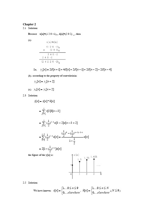
Chapter 22.1 Solution:Because x[n]=(1 2 0 –1)0, h[n]=(2 0 2)1-, then (a).So, ]4[2]2[2]1[2][4]1[2][1---+-+++=n n n n n n y δδδδδ(b). according to the property of convolutioin:]2[][12+=n y n y(c). ]2[][13+=n y n y2.3 Solution:][*][][n h n x n y =][][k n h k x k -=∑∞-∞=∑∞-∞=-+--=k k k n u k u ]2[]2[)21(2][211)21()21(][)21(12)2(0222n u n u n n k k --==+-++=-∑][])21(1[21n u n +-=the figure of the y[n] is:2.5 Solution:We have known: ⎩⎨⎧≤≤=elsewhere n n x ....090....1][,,, ⎩⎨⎧≤≤=elsewhere N n n h ....00....1][,,,(9≤N)Then, ]10[][][--=n u n u n x , ]1[][][---=N n u n u n h∑∞-∞=-==k k n u k h n h n x n y ][][][*][][∑∞-∞=-------=k k n u k n u N k u k u ])10[][])(1[][(So, y[4] ∑∞-∞=-------=k k u k u N k u k u ])6[]4[])(1[][(⎪⎪⎩⎪⎪⎨⎧≥≤=∑∑==4,...14, (14)N N k Nk =5, then 4≥NAnd y[14] ∑∞-∞=------=k k u k u N k u k u ])4[]14[])(1[][(⎪⎪⎩⎪⎪⎨⎧≥≤=∑∑==14,...114, (114)55N N k Nk =0, then 5<N∴ 4=N2.7 Solution:[][][2]k y n x k g n k ∞=-∞=-∑(a ) [][1]x n n δ=-,[][][2][1][2][2]k k y n x k g n k k g n k g n δ∞∞=-∞=-∞=-=--=-∑∑(b) [][2]x n n δ=-,[][][2][2][2][4]k k y n x k g n k k g n k g n δ∞∞=-∞=-∞=-=--=-∑∑(c) S is not LTI system.. (d) [][]x n u n =,0[][][2][][2][2]k k k y n x k g n k u k g n k g n k ∞∞∞=-∞=-∞==-=-=-∑∑∑2.8 Solution:)]1(2)2([*)()(*)()(+++==t t t x t h t x t y δδ)1(2)2(+++=t x t xThen,That is, ⎪⎪⎪⎩⎪⎪⎪⎨⎧≤<-≤<-+-=-<<-+=others t t t t t t t t y ,........010,....2201,.....41..,.........412,.....3)(2.10 Solution:(a). We know: Then, )()()(αδδ--='t t t h)]()([*)()(*)()(αδδ--='='t t t x t h t x t y)()(α--=t x t xthat is,So, ⎪⎪⎩⎪⎪⎨⎧+≤≤-+≤≤≤≤=others t t t t t t y ,.....011,.....11,....0,.....)(ααααα(b). From the figure of )(t y ', only if 1=α, )(t y ' would contain merely therediscontinuities.2.11 Solution:(a). )(*)]5()3([)(*)()(3t u e t u t u t h t x t y t ----==⎰⎰∞∞---∞∞--------=ττττττττd t u e u d t u eu t t )()5()()3()(3)(3⎰⎰-------=tt t t d e t u d et u 5)(33)(3)5()3(ττττ⎪⎪⎪⎪⎩⎪⎪⎪⎪⎨⎧≥+-=-<≤-=<=---------⎰⎰⎰5,.......353,.....313.........,.........0315395)(33)(3393)(3t e e d e d e t e d e t tt t t t t t t t ττττττ(b). )(*)]5()3([)(*)/)(()(3t u e t t t h dt t dx t g t----==δδ)5()3()5(3)3(3---=----t u e t u e t t(c). It ’s obvious that dt t dy t g /)()(=.2.12 Solution∑∑∞-∞=-∞-∞=--=-=k tk tk t t u ek t t u e t y )]3(*)([)3(*)()(δδ∑∞-∞=---=k k t k t u e)3()3(Considering for 30<≤t ,we can obtain33311])3([)(---∞=-∞-∞=--==-=∑∑e e e ek t u e e t y tk k tk kt.(Because k must be negetive , 1)3(=-k t u for 30<≤t ).2.19 Solution:(a). We have known: ][]1[21][n x n w n w +-=(1)][]1[][n w n y n y βα+-=(2)from (1), 21)(1-=E EE Hfrom (2), αβ-=E EE H )(2then, 212212)21(1)21)(()()()(--++-=--==E E E E E E H E H E H ααβαβ∴ ][]2[2]1[)21(][n x n y n y n y βαα=-+-+-but, ][]1[43]2[81][n x n y n y n y +-+--=∴ ⎪⎩⎪⎨⎧=⎪⎭⎫ ⎝⎛=+=143)21(:....812βααor∴⎪⎩⎪⎨⎧==141βα (b). from (a), we know )21)(41()()()(221--==E E E E H E H E H21241-+--=E E E E∴ ][)41()21(2][n u n h n n ⎥⎦⎤⎢⎣⎡-=2.20 (a). 1⎰⎰∞∞-∞∞-===1)0cos()cos()()cos()(0dt t t dt t t u δ(b). 0 dt t t )3()2sin(5+⎰δπ has value only on 3-=t , but ]5,0[3∉-∴dt t t )3()2sin(5+⎰δπ=0(c). 0⎰⎰---=-641551)2cos()()2cos()1(dt t t u d u πτπττ⎰-'-=64)2cos()(dt t t πδ0|)2(s co ='=t t π0|)2sin(20=-==t t ππ2.23 Solution:∑∞-∞=-==k t h kT t t h t x t y )(*)()(*)()(δ∑∞-∞=-=k kT t h )(∴2.27 Solution()y A y t dt ∞-∞=⎰,()xA x t dt ∞-∞=⎰,()hA h t dt ∞-∞=⎰.()()*()()()y t x t h t x x t d τττ∞-∞==-⎰()()()()()()()()()(){()}y x hA y t dt x x t d dtx x t dtd x x t dtd x x d d x d x d A A ττττττττττξξτττξξ∞∞∞-∞-∞-∞∞∞∞∞-∞-∞-∞-∞∞∞∞∞-∞-∞-∞-∞==-=-=-===⎰⎰⎰⎰⎰⎰⎰⎰⎰⎰⎰2.40 Solution(a) ()()(2)tt y t ex d τττ---∞=-⎰,Let ()()x t t δ=,then ()()y t h t =.So , 2()(2)(2)()(2)()(2)tt t t t h t ed e d e u t τξδττδξξ---------∞-∞=-==-⎰⎰(b) (2)()()*()[(1)(2)]*(2)t y t x t h t u t u t eu t --==+---(2)(2)(1)(2)(2)(2)t t u eu t d u e u t d ττττττττ∞∞-------∞-∞=+------⎰⎰22(2)(2)12(1)(4)t t t t u t ed u te d ττττ---------=---⎰⎰(2)2(2)212(1)[]|(4)[]|t t t t u t e e u t ee ττ-------=--- (1)(4)[1](1)[1](4)t t e u t e u t ----=-----2.46 SolutionBecause)]1([2)1(]2[)(33-+-=--t u dtde t u e dt d t x dt d t t)1(2)(3)1(2)(333-+-=-+-=--t e t x t et x tδδ.From LTI property ,we know)1(2)(3)(3-+-→-t h e t y t x dtdwhere )(t h is the impulse response of the system. So ,following equation can be derived.)()1(223t u e t h e t --=-Finally, )1(21)()1(23+=+-t u e e t h t 2.47 SoliutionAccording to the property of the linear time-invariant system: (a). )(2)(*)(2)(*)()(000t y t h t x t h t x t y ===(b). )(*)]2()([)(*)()(00t h t x t x t h t x t y --==)(*)2()(*)(0000t h t x t h t x --=)2()(00--=t y t y(c). )1()1(*)(*)2()1(*)2()(*)()(00000-=+-=+-==t y t t h t x t h t x t h t x t y δ(d). The condition is not enough.(e). )(*)()(*)()(00t h t x t h t x t y --== τττd t h x )()(00+--=⎰∞∞-)()()(000t y dm m t h m x -=--=⎰∞∞-(f). )()]([)](*)([)(*)()(*)()(000000t y t y t h t x t h t x t h t x t y "=''='--'=-'-'==Extra problems:1. Solute h(t), h[n](1). )()(6)(5)(22t x t y t y dt dt y dtd =++ (2). ]1[][2]1[2]2[+=++++n x n y n y n y012y(t)t4Solution:(1). Because 3121)3)(2(1651)(2+-++=++=++=P P P P P P P H so )()()()3121()(32t u e e t P P t h t t ---=+-++=δ (2). Because )1)(1(1)1(22)(22i E i E EE E E E E E H -+++=++=++=iE Ei i E E i -+-+++=1212so []][)1()1(2][1212][n u i i i k i E E i i E E i n h n n +----=⎪⎪⎪⎪⎭⎫⎝⎛-+-+++=δ。
(完整版)信号与系统奥本海姆_习题答案
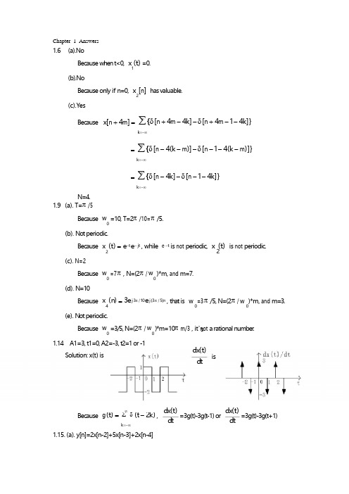
∑ {δ [n + 4m - 4k ] - δ [n + 4m - 1 - 4k ]}∑ {δ [n - 4(k - m )] - δ [n - 1 - 4(k - m )]}∑ {δ [n - 4k ] - δ [n - 1 - 4k ]}s Because g (t ) =∑ δ (t - 2k ) ,Chapter 1 Answers1.6 (a).NoBecause when t<0, x (t ) =0. 1(b).NoBecause only if n=0, x [n ] has valuable.2(c).Y esBecause x[n + 4m ] ===∞ k =-∞ ∞ k =-∞ ∞ k =-∞N=4.1.9 (a). T=π /5Because w =10, T=2π /10= π /5.(b). Not periodic.Because x (t ) = e -t e - jt , while e -t is not periodic, x (t ) is not periodic.2 2(c). N=2Because w =7 π , N=(2 π / w )*m, and m=7.0 0(d). N =10Because x (n) = 3e j 3π / 10 e j (3π / 5)n , that is w =3 π /5, N=(2 π / w )*m, and m=3.4 0(e). Not periodic.Because w =3/5, N=(2 π / w )*m=10π m/3 , it ’not a rational number .1.14 A1=3, t1=0, A2=-3, t2=1 or -1Solution: x(t) isdx(t )dtis∞ k =-∞1.15. (a). y[n]=2x[n-2]+5x[n-3]+2x[n-4]dx(t ) dx(t )=3g(t)-3g(t -1) or =3g(t)-3g(t+1)d t dt2 22 12Solution:y [n ] = x [n - 2] + 1x [n - 3] 2 2 1= y [n - 2] + y [n - 3]1 1= {2 x [n - 2] + 4 x [n - 3]} + {2 x [n - 3] + 4 x [n - 4]}1 1 1 1 =2 x [n - 2] + 5x [n - 3] + 2 x [n - 4]1 11Then, y[n ] = 2 x [n - 2] + 5x[n - 3] + 2 x [n - 4](b).No. For it ’s linearity .the relationship be tw e en y [n ] and x [n ] is the same in-out relationship with (a).1 2you can have a try.1.16. (a). No.For example, when n=0, y[0]=x[0]x[-2]. So the system is memory . (b). y[n]=0.When the input is A δ [n ] ,then, y[n] = A 2δ [n]δ [n - 2] , so y[n]=0.(c). No.For example, when x[n]=0, y[n]=0; when x[n]= A δ [n ] , y[n]=0.So the system is not invertible.1.17. (a). No.For example, y(-π ) = x(0) . So it ’s not causal.(b). Y es.Because : y (t ) = x (sin(t )) ,y (t ) = x (sin(t ))1 122ay (t ) + by (t ) = ax (sin(t )) + bx (sin(t ))1 2121.21. Solution:W e(a).have known:(b).(c).(d).1.22.Solution:W e have known:(a).(b).(e).22 E {x(t )} =(g)1.23. Solution:For1[ x (t ) + x(-t )] v 1O {x(t )} = [ x (t ) - x(-t )] dthen, (a).(b).(c).1.24.2Solution:For:E {x[n ]} = v 1 2( x [n ] + x[-n ])1O {x[n]} = ( x [n ] - x[-n ]) dthen,(a).(b).Solution: x(t ) = E {cos(4π t )u(t )}s(c).1.25. (a). Periodic. T=π /2.Solution: T=2π /4= π /2. (b). Periodic. T=2.Solution: T=2π / π =2. (d). Periodic. T=0.5.v1= {cos(4πt )u (t ) + cos(4π (-t ))u (-t )}2 1= cos(4π t ){u (t ) + u(-t )}2 1= cos(4π t )2So, T=2π /4 π =0.51.26. (a). Periodic. N=7Solution: N= 2π* m =7, m=3.6π / 7(b). Aperriodic.Solution: N= 2π 1/ 8* m = 16m π , it ’not rational number .(e). Periodic. N =16Solution as follow:2 cos( n ) , it ’s period is N=2π *m/( π /4)=8, m=1.sin( n ) , it ’s period is N=2π *m/( π /8)=16, m=1.(2). g (t ) ∑δ (t - 2k )π π π πx[n ] = 2 cos( n ) + sin( n ) - 2 cos( n + 4 8 2 6)in this equation,π4 π8π π- 2 cos( n + 2 6) , it ’s period is N=2π *m/( π /2)=4, m=1.So, the fundamental period of x[n ] is N=(8,16,4)=16.1.31. SolutionBecausex (t ) = x (t ) - x (t - 2), x (t ) = x (t + 1) + x (t ) .2 11311According to LTI property ,y (t ) = y (t ) - y (t - 2), y (t ) = y (t + 1) + y (t )2 11311Extra problems:1. SupposeSketch y(t ) = ⎰t-∞x(t )dt .Solution:2. SupposeSketch:(1). g (t )[δ (t + 3) + δ (t + 1) - 2δ (t - 1)]∞k =-∞Because x[n]=(1 2 0 –1) , h[n]=(2 0 2) , the nSolution: (1).(2).Chapter 22.1 Solution:-1(a).So,y [n ] = 2δ [n + 1] + 4δ [n ] + 2δ [n - 1] + 2δ [n - 2] - 2δ [n - 4]1(b). according to the property of convolutioin:y [n ] = y [n + 2]2 1(c). y [n] = y [n + 2]31=∑ x[k ]h [n - k ]( ) 0 - ( ) (n +2)-2+1= ∑ ( ) k -2 u[n] = 2 u[n]2 ⎩0, elsewhere W e have known: x[n] = ⎨ ⎩0,elsewhere , h[n] = ⎨ ,( N ≤ 9 ), , ∑ h[k ]u[n - k ]∑ (u[k ] - u[k - N - 1])(u[n - k ] - u[n - k - 10])∑ (u[k ] - u[k - N - 1])(u[4 - k ] - u[-k - 6])⎧∑ 1,...N ≤ 4⎪∑1,...N ≥ 4 ⎪⎩∑ (u[k ] - u[k - N - 1])(u[14 - k ] - u[4 - k ])2.3 Solution:y[n ] = x[n ]* h [n ]∞ k =-∞ ∞1= ∑ ( ) k -2 u [k - 2]u [n - k + 2]2k =-∞1 1 n +2 121 k =2 1 -21= 2[1 - ( ) n +1 ]u [n ]2the figure of the y[n] is:2.5 Solution:⎧1 ....0 ≤ n ≤ 9 ....⎧1 0≤ n ≤ N .... Then,x[n] = u[n] - u[n - 10] , h[n] = u[n] - u[n - N - 1]y[n] = x[n]* h[n] =∞k =-∞=∞ k =-∞So, y[4] =∞ k =-∞N⎪ ⎪ = ⎨k =04k =0=5, the n N ≥ 4And y[14] =∞ k =-∞⎧∑ 1,...N ≤ 14⎪∑1,...N ≥ 14 ⎪⎩ ∑ x[k ]g [n - 2k ]∑ x[k ]g [n - 2k ] = ∑ δ [k - 1]g [n - 2k ] = g [n - 2]∑ x[k ]g [n - 2k ] = ∑ δ [k - 2]g [n - 2k ] = g [n - 4]∑ x[k ]g [n - 2k ] = ∑ u[k ]g [n - 2k ] = ∑ g [n - 2k ]N⎪ ⎪= ⎨ k =514k =5∴N = 4=0, the n N < 52.7 Solution:y[n] =∞k =-∞(a ) x[n] = δ [n - 1] , y[n] =∞∞k =-∞ k =-∞ (b)x[n] = δ [n - 2] , y[n] =∞∞k =-∞k =-∞(c) S is not LTI system..(d) x[n] = u[n] , y[n] =∞ ∞∞k =-∞k =-∞ k =02.8 Solution:y(t ) = x(t ) * h (t ) = x(t ) *[δ (t + 2) + 2δ (t + 1)]= x(t + 2) + 2 x (t + 1)Then,⎩ = ⎰ u(τ - 3)e -3(t -τ )u(t - τ )d τ - ⎰ u(τ - 5)e -3(t -τ )u(t - τ )d τ⎩= u(t - 3)⎰ e -3(t -τ ) d τ - u(t - 5)⎰ e -3(t -τ ) d τ⎧t + 3,..... - 2 < t < -1 ⎪4,.......... t = -1 ⎪⎪That is, y(t ) = ⎨t + 4,..... - 1 < t ≤ 0⎪2 - 2t,....0 < t ≤ 1 ⎪ ⎪0,....... others2.10 Solution:(a). W e know:Then,h '(t ) = δ (t ) - δ (t - α )y '(t ) = x(t ) * h '(t ) = x(t ) *[δ (t ) - δ (t - α )]= x(t ) - x(t - α )that is,⎧t,.....0 ≤ t ≤ α ⎪α ,....α ≤ t ≤ 1So, y(t ) = ⎨⎪1 + α - t,.....1 ≤ t ≤ 1 + α ⎪0,.....others(b). From the figure of y '(t ) , only if α = 1 , y '(t ) would contain merely therediscontinuities.2.11 Solution:(a).y(t ) = x(t ) * h(t ) = [u (t - 3) - u (t - 5)]* e -3t u (t )∞ ∞-∞-∞tt35= ⎨⎰ e -3(t -τ ) d τ = ,.....3 ≤ t < 5 ⎪ 3 ⎪⎰ e -3(t -τ ) d τ - ⎰ e -3(t -τ ) d τ = - e ⎪ t9-3t + e 15-3t ⎪⎩ s y(t ) = e -t u (t ) * ∑ δ (t - 3k ) = ∑ [e = ∑ e -(t -3k )u (t - 3k )y(t ) = e -t [ ∑ e 3k u (t - 3k )] = e -t∑ ew [n ] = 1w [n - 1] + x[n ]⎧⎪ ⎪0,................. t < 3⎪ t1 - e 9-3t3t353,...... t ≥ 5(b). g (t ) = (dx(t ) / dt ) * h(t ) = [δ (t - 3) - δ (t - 5)]* e -3t u (t )= e -3(t -3) u (t - 3) - e -3(t -5) u (t - 5)(c). It ’obvious that g (t ) = d y (t ) / dt .2.12 Solution∞∞k =-∞k =-∞∞k =-∞Considering for 0 ≤ t < 3 ,we can obtain-t u (t ) * δ (t - 3k )]∞k =-∞0 k =-∞3k= e -t 11 - e -3.(Because k mu st be negetive , u (t - 3k ) = 1 for 0 ≤ t < 3 ).2.19 Solution:(a). W e have known:2 (1)y[n ] = αy[n - 1] + βw [n ](2)then, H ( E ) = H ( E ) H ( E ) =βE 2= .... or : (α + ) = ∴⎨ 2 8 ⎝ 2 = - E ∴ h [n ] = ⎢2( ) n - ( ) n ⎥u [n ] ⎩Θ⎰⎰ sin(2πt )δ (t + 3)dt has value only on t = -3 , but - 3 ∉ [0,5]⎰ sin(2πt )δ (t + 3)dt =0Θ⎰-4from (1), H ( E ) =E1E -1 2from (2), H ( E ) =2 βEE - α121 ( E - α )(E - )2 = β1 α 1 - (α + ) E -1 + E -22 21 α∴ y[n ] - (α + ) y[n - 1] + y[n - 2] = βx[n ]2 21 3but, y[n ] = - y[n - 2] + y[n - 1] + x[n ]8 4⎧α 1 ⎛1 ⎪ 3 ⎫ ⎪4 ⎭ ⎧ 1 ⎪α = ∴⎨ 4⎪β = 1(b). from (a), we know H ( E ) = H ( E ) H ( E ) =1 22E +1 1 E - E -4 2⎡ 1 1 ⎤ ⎣ 24 ⎦2.20 (a). 1⎪⎩β = 1E 21 1 ( E - )(E - ) 4 2(b). 0∞-∞ u (t ) cos(t )dt =⎰∞ δ (t ) cos(t )dt = cos(0) = 1-∞Θ∴(c). 05 0 5 05-5 u (1 - τ ) cos(2πτ )d τ = -⎰6 u (t ) cos(2πt )dt1 1= -⎰6 δ '(t ) cos(2πt )dt-4= cos '(2π t ) |t =0= -2π sin(2πt ) |t =0= 0∑ δ (t - kT ) * h (t )∑ h (t - kT )⎰ y(t )d t , A = ⎰ x(t )dt ,A = ⎰ h(t )d t .⎰ x(τ ) x (t - τ )d τ⎰ y(t )dt = ⎰ ⎰ x(τ ) x (t - τ )d τd t= ⎰ ⎰ x(τ ) x (t - τ )dtd τ = ⎰ x(τ ) ⎰ x(t - τ )dtd τ⎰ x(τ ) ⎰ x(ξ )d ξ d τ = ⎰ x(τ )d τ{ ⎰ x(ξ )d ξ}2.23 Solution:Θ y(t ) = x(t ) * h (t ) =∞k =-∞=∞ k =-∞∴2.27 SolutionA = y∞ ∞ ∞ x h-∞ y(t ) = x(t )* h(t ) = -∞ -∞ ∞-∞A = y∞ ∞ ∞-∞ -∞ -∞∞ ∞∞∞-∞ -∞-∞ -∞= ∞ ∞ ∞ ∞-∞= A Ax h-∞ -∞ -∞⎰e ⎰ eδ (τ - 2)d τ = ⎰ e⎰ u(τ + 1)eu(t - 2 - τ )d τ - ⎰ u(τ - 2)e= u(t - 1) ⎰ ed τ - u(t - 4) ⎰ e-(t -2-τ )d τ2.40 Solution(a) y(t ) = t-(t -τ) x(τ - 2)d τ ,Let x(t ) = δ (t ) ,then y(t ) = h (t ) .-∞So , h(t ) = t t -2-(t -τ ) -∞-∞-(t -2-ξ )δ (ξ )d ξ = e -(t -2)u(t - 2)(b)y(t ) = x(t )* h(t ) = [u(t + 1) - u(t - 2)]* e -(t -2)u(t - 2)=∞ ∞ -(t -2-τ )-∞-∞-(t -2-τ )u(t - 2 - τ )d τt -2-1-(t -2-τ ) t -2 2= u(t - 1)[e -(t -2) e τ ]| t -2 -u(t - 4)[e -(t -2) e τ ]| t -2-1 2= [1- e -(t -1) ]u(t - 1) - [1- e -(t -4) ]u(t - 4)2.46 SolutionBecaused d dx(t ) = [ 2e -3t ]u (t - 1) + 2e -3t [ u (t - 1)] d t dt d t= -3x(t ) + 2e -3t δ (t - 1) = -3x(t ) + 2e -3δ (t - 1) .From LTI property ,we knowdd tx(t ) → -3 y (t ) + 2e -3 h (t - 1)whereh (t ) is the impulse response of the system.So ,following equation can be derived.2e -3h(t - 1) = e -2t u (t )Finally, h (t ) = 12e 3e -2(t +1)u (t + 1)2.47 SoliutionAccording to the property of the linear time-invariant system:(a). y(t ) = x(t ) * h(t ) = 2 x (t ) * h (t ) = 2 y (t )0 0(b). y(t ) = x(t ) * h(t ) = [ x (t ) - x (t - 2)]* h(t )1y(t)= x (t ) * h (t ) - x (t - 2) * h (t )0 2 4t= [ y (t )] = y (1). Because H ( P ) = 1so h (t ) = (1= 2 + E - E ⎪ [ ]⎪δ [k ] = i (-1 - i) n- (-1 + i) n u [n] so h [n ] = 2 2 i= y (t ) - y (t - 2)0 0(c). y(t ) = x(t ) * h(t ) = x (t - 2) * h (t + 1) = x (t - 2) * h (t ) * δ (t + 1) = y (t - 1)0 0(d). The condition is not enough.(e). y(t ) = x(t ) * h(t ) = x (-t ) * h (-t )0 0= ⎰∞ x (-τ )h (-t + τ )d τ-∞ = ⎰∞x (m )h (-t - m )dm = y (-t )-∞(f). y(t ) = x(t ) * h (t ) = x ' (-t ) * h ' (-t ) = [ x ' (-t ) * h (-t )] ' ' ' " (t )Extra problems:1. Solute h(t), h[n](1). d 2 dy(t ) + 5 y(t ) + 6 y(t ) = x(t )dt 2 dt(2). y[n + 2] + 2 y[n + 1] + 2 y[n ] = x[n + 1]Solution:1 1 - 1= = +P 2 + 5P + 6 ( P + 2)( P + 3) P + 2 P + 3- 1+)δ (t ) = (e -2t - e -3t )u (t )P + 2P + 3(2). Because H ( E ) = E E E= =E 2 + 2E + 2 ( E + 1) 2 + 1 ( E + 1 + i)( E + 1 - i)i i E - E2E + 1 + i E + 1 - i⎛ i ⎫+E + 1 + i E + 1 - i ⎪ 2 ⎪ ⎝ ⎭x(t ) = ∑ for the period of cos( 5πt ) is T = 63the period of sin( 22⎰ x 2 (t )e - jkw 2t d t = ⎰ ( x 1 (1- t ) + x 1 (t - 1))e - jkw 1t dtT T TChapter 33.1 Solution:Fundamental period T = 8 . ω = 2π / 8 = π / 4∞a e j ω0kt = a e j ω0t + a e - j ω0t + a e j 3ω0t + a e - j 3ω0tk 1 -1 3 -3k =-∞ = 2ej ω0t+ 2e - j ω0t + 4 je j 3ω0t - 4 je - j3ω0t π 3π= 4cos( t ) - 8sin( t )4 43.2 Solution:for , a = 1 , a0 -2= e - j π / 4 , a = e j π / 4 , a 2-4= 2e - j π / 3 , a = 2e j π / 34x[n] = ∑ a e jk (2π / N )nkk =< N >= a + a e j (4π / 5)n + a e - j (4π / 5)n + a e j (8π / 5)n + a e - j (8π / 5)n0 2-24-4= 1 + e j π / 4 e j (4π / 5)n + e - j π / 4 e - j (4π / 5)n + 2e j π / 3e j (8π / 5)n + 2e - j π / 3e - j (8π / 5)n4 π 8 π= 1 + 2 cos( πn + ) + 4 cos( πn + )5 4 5 3 4 3π 8 5π= 1 + 2sin( πn + ) + 4sin( πn + )5 4 5 63.3 Solution:2πt ) is T= 3 , 3so the period of x(t ) is 6 , i.e. w = 2π / 6 = π / 32π 5π x(t ) = 2 + cos(t ) + 4sin(t )331= 2 + cos(2w t ) + 4sin(5w t )0 0 1= 2 + (e j 2w 0t + e - j 2w 0t ) - 2 j(e j5w 0t - e - j5w 0t )2 then, a = 2 , a 0 -2 1= a = , a 2 -5 = 2 j , a = -2 j 53.5 Solution:(1). Because x (t ) = x (1 - t ) + x (t - 1) , the n x (t ) has the same period as x (t ) ,21121that is T = T = T ,w = w2121(2). b = 1 k⎰ x 1 (1- t )e - jkw 1t d t + 1 ⎰ x 1 (t - 1)e - jkw 1t dt ∑∑⎰ x(t ) 2 dt = a 0 2 + a -1 2 + a 1 2 = 2 a 1 2 = 1 Fundamental period T = 8 . ω = 2π / 8 = π / 4∑∑ a H ( jkw )ejkw 0tk ω ⎩0,......k ≠ 0⎧ ∑t Because a =⎰ x(t )d t = 1⎰4 1d t + 1 ⎰ 8(-1)d t = 0TT88 4= 1 T T T T= a e - jkw 1 + a e - jkw 1 = (a -k k3.8 Solution:-k+ a )e - jkw 1 kΘx(t ) =∞ k =-∞a e jw 0ktkwhile:andx(t ) is real and odd, the n a = 0 , a = -a 0 kT = 2 , the n w = 2π / 2 = πa = 0 for k > 1k-ksox(t ) =∞ a e jw 0kt = a + a e - jw 0t + a e jw 0tk 0 -1 1k =-∞= a (e j πt - e - j πt ) = 2a sin(π t )11for1 2 2 0∴∴a = ± 2 /21x(t ) = ± 2 sin(π t )3.13 Solution:Θx(t ) =∞ k =-∞a e jw 0ktk∴ y(t ) =∞k 0k =-∞H ( jk ω ) = sin(4k ω0 ) =⎨4,...... k = 00 0 ∴ y(t ) =∞a H ( jkw )e jkw 0= 4a k 00 k =-∞1Soy(t ) = 0 .∑∑a H(jkw)e jkw0tT t H(jw)=⎨if a=0,it needs kw>100T ⎰T⎰t dt=0T ⎰x(t)e-jkw0t dt=⎰te-jk22t dt=1⎰1te-jkπt dt11⎰1tde-jkπt2jkπ⎢-1⎦⎢(e-jkπ+e jkπ)-⎥-jkπ2c os(kπ)+-jkπ⎥⎦[2cos(kπ)]=j cos(kπ)=j(-1)k............k≠03.15Solution:Θx(t)=∞k=-∞a e jw0kt k∴y(t)=∞k=-∞k0∴a=1k ⎰Ty(t)H(jkw)e-jkw0d tfor⎧⎪1,......w≤100⎪⎩0,......w>100∴k0that is k2π100 >100,.......k>π/612and k is integer,so K>8 3.22Solution:a=10x(t)dt=112-1a= k 1T2-12-1π=-1 2jkπ-1=-1⎡⎢te-jkπt⎣1-1-e-jkπt-jkπ1⎤⎥⎥=-=-12jkπ12jkπ⎡(e-jkπ-e jkπ)⎤⎣⎦⎡2sin(kπ)⎤⎢⎣=-12jkπkπkπ⎰ h (t )e - j ωt d t = ⎰ e -4 t e - j ωt d t= ⎰ e e d t + ⎰ e -4t e - j ωt d t∑0 ∑∑Ta = ⎰ x(t )e - jkw 0t d t = ⎰1/ 2 δ(t )e - jk 2πt d t = 1T T-1/ 2 ∑T∑ (-1) δ (t - n ) .T=2, ω = π , a = 1T a = ⎰ x(t )e - jkw 0t d t = ⎰ δ (t )e - jk πt d t + ⎰ 3/ 2 (-1)δ (t - 1)e - jk πt d tT 2 -1/ 2 2 1/ 2 T 16 + (k π )23.34 Solution:∞ ∞H ( j ω ) =-∞-∞0 ∞ 4t - j ωt-∞118=+=4 - j ω 4 + j ω 16 + ω 2A periodic continous-signal has Fourier Series:. x(t ) =T is the fundamental period of x(t ) . ω = 2π / T∞ k =-∞a e j ω ktkThe output of LTI system with inputed x(t ) is y(t ) =Its coefficients of Fourier Series: b = a H ( jk ω )k k 0∞ k =-∞a H ( jk ω )e jk ω tk 0(a) x(t ) =∞ n =-∞ δ (t - n ) .T=1, ω = 2π a = 1 = 1 .0 k1 k(N ot e :If x(t ) =∞ n =-∞δ (t - nT ) , a =1 k)So b = a H ( jk 2π ) = k k 8 2=16 + (2k π )2 4 + (k π )2(b) x(t ) = ∞n =-∞n0 k= 11 1 1/2 1 k1= [1- (-1)k ] 24[1-(-1)k ]So b = a H ( jk π ) = ,k k(c) T=1, ω = 2π⎰ x(t )e - jk ω0t d t = ⎰1/ 4e - jk 2πt d t =∑∑ a H ( jkw )ejkw 0t⎪⎩0,......otherwise ⎩0,......otherwise H ( jw) = ⎨⎪, 14Let y(t ) = x(t ) , b = a , it needs a = 0 ,for k < 18..or .. k ≤ 17 .∑∑∑ 2n e - j ωn + ∑ ( )n e - j ωn1 =2 41 1 5∑a ejk ( N )n .a = k1 T T -1/ 4 k π sin(2 k π)b = a H ( jk π ) =k k k π8sin( )2 k π [16 + (2k π )2 ]3.35 Solution: T= π / 7 , ω = 2π / T = 14 .Θx(t ) =∞a e jw 0ktk∴y(t ) =k =-∞ ∞ k =-∞k 0∴b = a H ( jkw )k k 0for ⎧1,...... w ≥ 250 ⎧1,...... k ≥ 170 that is k ω 0 < 250,....... k < 250, and k is integer , so k < 18..or .. k ≤ 17 .kkk3.37 Solution:H (ej ω) = ∞n =-∞h [n ]e- j ωn=∞ n =-∞1 ( ) ne - j ωn 2-1∞1= 2n =-∞ n =0 1 3e j ω+ =1 - e j ω 1 - e - j ω - cos ω2 2 4A periodic sequen ce has Fourier Series: x [n ] =N is the fundamental period of x[n ] .k =< N >k2πThe output of LTI system with inputed x[n ] is y[n ] =∑ a H (ekj 2π k N)ejk ( 2π )n N .k =< N >∑4 .So b = a H (e j N k ) = 1 4 45 - cos( 2π k ) k =2 21 T ' 1 3T '-1 = ⎰ x(3t - 1)e T ' dt = ⎰ x(m )e = ⎰ x(m )e e⎡ 1T -1 T ⎢⎰∑a e jk (2π/T )t ,where a = 0 for every2π Its coefficients of Fourier Series: b = a H (ejN k )kk3(a) x[n ] =∞ k =-∞δ [n - 4k ] .N=4, a = 1 k k k 2π 4 4b =k3 165 π- cos( k ) 4 23.40 Solution:According to the property of fourier series:(a). a k '= a e - jkw 0t 0 + a e jkw 0t 0 = 2a cos(kw t ) = 2a cos(k k k k 0 0 k 2π t )T 0(b). Because E {x(t )} =v x(t ) + x(-t )2a ' a + a k 2-k= E {a }v k(c). Because R {x(t )} = x(t ) + x * (t )e'a + a *a = k-k k(d). a '= ( jkw ) 2 a = ( jk k 0 k 2πT) 2 ak(e). first, the period of x(3t - 1) is T ' =T3th e n ak ' 2π - jk t T ' 0 T ' -11 T -12π 2π - jkm - jk dmT TT -1- jk 2π m +1 dm T ' 3 3= e- jk 2π ⎣ T -1x(m )e2π- jk m T⎤dm ⎥⎦2π = a e- jk Tk3.43 (a) Proof:( i ) Because x(t ) is odd harmonic , x(t ) =non-zer o even k.∞ k =-∞k kx(t + ) = ∑ a e jk (2π /T )(t + 2 )T 2∑= - ∑ a e jk (2π /T )t(ii )Because of x(t ) = - x (t + ) ,we get the coefficients of Fourier Seriesa = ⎰ x(t )e - jk 2T π t d t = 1 ⎰ T / 2 x(t )e - jk 2T π t d t + 1 ⎰ T x(t )e - jk 2T π t d tT 0 T 0 T T /2 1 T /2 1 T /2 = ⎰ T dt + ⎰ x(t + T / 2)e x(t )e 1 T /2 1 T /2 = ⎰ x(t )eT dt - ⎰ x(t )(-1)k e T dt 1T /2It is obvious that a = 0 for every non-zer o even k. So x(t ) is odd harmonic ,-11x(t ) = ∑ δ (t - kT ) , T = π∞ T k k =-∞= ∞a e jk π e jk (2π /T )tkk =-∞∞kk =-∞It is noticed that k is odd integers or k=0.That meansTx(t ) = - x (t + )2T21 T k2π - jk t T 0 T 0 2π- jk (t +T / 2) Tdt2π 2π- jk t - jk t T 0 T 0= [1- (-1)k ] ⎰T 02π x(t )e- jk Tt d tk(b) x(t )1......-2-12 tExtra problems:∞ k =-∞(1). Consider y(t ) , when H ( jw) isx(t ) = ∑ δ (t - kT ) ↔T π T∑ a H ( jkw )ejkw 0t=1k =-∞ π∑∑π∑1(2). Consider y(t ) , when H ( jw) isSolution:∞k =-∞ 1 1 2π= , w = = 2 0(1).y(t ) =∞k 0∞k =-∞a H ( j 2k )e j 2ktk=2π (for k can only has value 0)(2).y(t ) =∞ k =-∞a H ( jkw )e jkw 0t =1k 0∞k =-∞a H ( j 2k )e j 2ktk=1π (e - j 2t + e j 2t ) =2 cos 2tπ(for k can only has value – and 1)。
- 1、下载文档前请自行甄别文档内容的完整性,平台不提供额外的编辑、内容补充、找答案等附加服务。
- 2、"仅部分预览"的文档,不可在线预览部分如存在完整性等问题,可反馈申请退款(可完整预览的文档不适用该条件!)。
- 3、如文档侵犯您的权益,请联系客服反馈,我们会尽快为您处理(人工客服工作时间:9:00-18:30)。
Heide Gluesing-Luerssen∗
arXiv:cs/0501016v1 [cs.IT] 10 Jan 2005
December 15, 2004
Abstract Detailed information about the weight distribution of a convolutional code is given by the adjacency matrix of the state diagram associated with a controller canonical form of the code. We will show that this matrix is an invariant of the code. Moreover, it will be proven that codes with the same adjacency matrix have the same dimension and the same Forney indices and finally that for one-dimensional binary convolutional codes the adjacency matrix determines the code uniquely up to monomial equivalence.
ห้องสมุดไป่ตู้
Keywords: Convolutional coding theory, controller canonical form, weight distribution, monomial equivalence, MacWilliams duality MSC (2000): 94B05, 94B10, 93B15
University of Groningen, Department of Mathematics, P. O. Box 800, 9700 AV Groningen, The Netherlands; gluesing@math.rug.nl
∗
1
of the state diagram associated with the controller canonical form of a minimal encoder. Since for block codes this matrix reduces to the usual weight distribution, it can be regarded as a generalization of the latter to convolutional codes. Then the following issues arise. First of all, it needs to be clarified whether this matrix is an invariant of the code, i. e., does not depend on the choice of the minimal encoder. Since at any rate the adjacency matrix depends on the chosen ordering on the state space, it is reasonable to factor out the effect of the ordering. This brings us to the notion of generalized adjacency matrix for which then we can answer the question above in the affirmative in Section 4. Secondly and more interestingly, we will approach the problem of how much information about the code does the generalized adjacency matrix contain. More precisely, what is the relation between two codes sharing the same generalized adjacency matrix? In Section 5 we will first show that two such codes always have the same Forney indices. Thereafter, we will restrict ourselves to the most important class of convolutional codes from a practical point of view, the one-dimensional binary codes. With the aid of MacWilliams’ Equivalence Theorem for block codes we will show that such codes share the same generalized adjacency matrix if and only if they are monomially equivalent. One should bear in mind that this result cannot be expected for general codes, since it is not even true for higher-dimensional binary block codes. However, as a consequence we obtain that if two binary one-dimensional convolutional codes share the same generalized adjacency matrix then so do their dual codes. This shows in particular that the example in [21] mentioned above does not apply if we consider the generalized adjacency matrix rather than the weight distribution of the atomic codewords. The result just mentioned tempts us to conjecture that two codes have the same generalized adjacency matrix if and only if this is true for the dual codes, or, more explicitly, that there might be a MacWilliams duality for the generalized adjacency matrices of convolutional codes. Indeed, in [1] in a totally different form a MacWilliams tranformation rule has been established for convolutional codes of the smallest kind, that is, with overall constraint length being one. We will present this transformation in (5.2) at the end of this paper. Proving or disproving the conjecture for general codes, however, appears to be quite a difficult problem and has to remain open for future research. In the next two sections we will introduce the material as necessary for deriving our results. We will discuss the controller canonical form of an encoder matrix and the associated state diagram along with its adjacency matrix. This will in particular bring us to a statespace description of convolutional codes as introduced first by Massey and Sain [12] and discussed in many other papers, see, e. g., [4, 13]. Since the results as we will need them later on are somewhat spread over the literature and proofs are not always easily accessible, we think it is worthwhile presenting the material of the next two sections as self-contained as possible, even though most of the results are not new. Furthermore, as opposed to the existing literature we will give a purely matrix theoretic approach. Following McEliece [14] we will introduce the notions of atomic and molecular codewords and show how the corresponding weight distribution can be derived, theoretically, from the adjacency matrix of the state diagram. Other methods of computing the weight distribution are Viterbi’s method, see [22] or [8, Sec. 3.10], or Mason’s gain formula as described in [10, Sec. 10.2]. For us McEliece’s approach has the advantage to be fully in matrix theoretic terms. This way we will obtain a consistent presentation throughout the whole paper which also bears the hope that we can bring this interesting topic closer to the mathematical community. Moreover, his method leads us directly to the adjacency matrix which will be the central object of our studies in the last two sections. At the end of Section 3, we will also briefly discuss two types of distance