
托马斯微积分课件4.6 Substitution in Definite Integrals
(定积分换元法)
目录
上页
下页
返回
结束
Proof. Let F denote any antiderivative of f
目录
上页
下页
返回
结束
Solution 1.
Solution 2.
目录
上页
下页
返回
结束
Example. Evaluate the integrals
Solution.
目录
上页
目录
上页
下页
返回
结束
目录
上页
下页
返回
结束
Example. Evaluate the area of the shade region.
目录
上页
下页
返回
结束
Example. Evaluate the area of the shade region.
目录
上页
下页
返回
结束
Exercises
P371 1(a), 4(a), 5(a), 6(a), 8(a), 12, 15. P372 19, 24.
Step 2. Select some number in each subinterval, and then obtain many rectangles.
目录
上页
下页
返回
结束
Step 3. Take the sum of above products.
Step 4. Take the limitation of Riemann sum.
下页
返回
结束
Example. Evaluate the integrals
Solution.
目录
上页
下页
返回
结束
4.6.2
Area between Curves (曲线之间的平面图形面积)
目录
上页
下页
返回
结束
目录
上页
下页
返回
结束
Step 1. Subdivide the interval [a,b] into subintervals.
Chapter 4 Integration
4.1 Indefinite Integrals, Differential Equations, and Modeling 4.2 Integral Rules, Integration by Substitution 4.3 Estimating with Finite Sums
that both f and g are continuous. Therefore, we have
目录
上页
下页
返回
结束
目录
上页
下页
返回
结束
Solution.
目录
上页
下页
返回
结束
Solution 1.
目录
上页
下页
返回
结束
Solution 2.
Does it has other Solutions?
下页
返回
结束
4.6
Substitution in Definite Integrals
目录
上页
下页
返回
结束
4.6.1 Substitution in Definite Integral 4.6.2 Area between Curves
目录
上页
下页
返回
结束
4.6.1
Substitution in Definite Integral
4.4 Riemann Sums and Definite Integrals 4.5 The Mean Value and Fundamental Theorems
4.6 Substitution in Definite Integrals 4.7 Numerical Integration
目录
上页
目录 上页 下页 返回 结束
Example. Evaluate the area of the shade region.
目录
上页
下页
返回
结束
Example. Evaluate the area of the shade region.
目录
上页
下页
返回
结束
Example. Evaluate the area of the shade region.
合集下载
微积分基本公式PPT学习教案

第12页/共62页
例9. 设 f (x, y) xy et2 dt, 求 0
x y
2 f x2
2 2 f xy
y x
2 f y 2
.
解:令 (s) s et2 dt, 则 '(s) es2 , f (x, y) (xy) 0
于是
f (xy) '(xy) xy' ex2y2 y
e x x2 y2
2x3 yex2y2
最终结果 2ex2 y2
第14页/共62页
例5 .
lim
x0
0 sin t 2dt
2x
x3
0 sin t 2dt '
lim 2x
x0 (x3 )'
lim
x0
s in(2 x ) 2 3x 2
(2 x )'
2 3
lim
x0
sin 4x x2
2
8 3
b( x)
f (t)dt
的导数 F( x) 为
a( x)
F( x) d
b( x)
f (t )dt
dx a( x)
f b( x)b( x)
f a( x)a( x)
证 F( x) 0 b( x) f (t)dt
a(x) 0
b( x) f (t )dt
a( x)
f (t)dt,
202
1
1 1 (2 2 1 1) 1
2
2
第20页/共62页
例10 计算
2
f (x)dx, 其中
0
2x,
f
(
x)
5,
0 x1 1 x 2
解
2
托马斯微积分
Chapter 2 ET. Finney Weir Giordano, Thomas’ Calculus, Tenth Edition © 2001. Addison Wesley Longman All rights reserved. Chapter 2ET, Slide 10
Figure 2.43: The balloon in Example 3.
Chapter 2 ET. Finney Weir Giordano, Thomas’ Calculus, Tenth Edition © 2001. Addison Wesley Longman All rights reserved. Chapter 2ET, Slide 7
Figure 2.31: sin (x°) oscillates only /180 times as often as sin x oscillates. Its maximum slope is /180. (Example 9)
Chapter 2 ET. Finney Weir Giordano, Thomas’ Calculus, Tenth Edition © 2001. Addison Wesley Longman All rights reserved. Chapter 2ET, Slide 15
Figure 2.51: The position of the curve y = (a h – 1) /h, a > 0, varies continuously with a.
Chapter 2 ET. Finney Weir Giordano, Thomas’ Calculus, Tenth Edition © 2001. Addison Wesley Longman All rights reserved. Chapter 2ET, Slide 16
Figure 2.43: The balloon in Example 3.
Chapter 2 ET. Finney Weir Giordano, Thomas’ Calculus, Tenth Edition © 2001. Addison Wesley Longman All rights reserved. Chapter 2ET, Slide 7
Figure 2.31: sin (x°) oscillates only /180 times as often as sin x oscillates. Its maximum slope is /180. (Example 9)
Chapter 2 ET. Finney Weir Giordano, Thomas’ Calculus, Tenth Edition © 2001. Addison Wesley Longman All rights reserved. Chapter 2ET, Slide 15
Figure 2.51: The position of the curve y = (a h – 1) /h, a > 0, varies continuously with a.
Chapter 2 ET. Finney Weir Giordano, Thomas’ Calculus, Tenth Edition © 2001. Addison Wesley Longman All rights reserved. Chapter 2ET, Slide 16
Functionals and stocpresentation of martingales Rama Cont泛函Ito微积分与鞅的随机积分表示(英文版)

Keywords: stochastic calculus, functional calculus, Ito formula, integration by parts, Malliavin derivative, martingale representation, semimartingale, Wiener functionals, functional Feynman-Kac formula, Kolmogorov equation, Clark-Ocone formula.
2
1
Introduction
Ito’s stochastic calculus [15, 16, 8, 24, 20, 28] has proven to be a powerful and useful tool in analyzing phenomena involving random, irregular evolution in time. Two characteristics distinguish the Ito calculus from other approaches to integration, which may also apply to stochastic processes. First is the possibility of dealing with processes, such as Brownian motion, which have non-smooth trajectories with infinite variation. Second is the non-anticipative nature of the quantities involved: viewed as a functional on the space of paths indexed by time, a non-anticipative quantity may only depend on the underlying path up to the current time. This notion, first formalized by Doob [9] in the 1950s via the concept of a filtered probability space, is the mathematical counterpart to the idea of causality. Two pillars of stochastic calculus are the theory of stochastic integration, which allows to T define integrals 0 Y dX for of a large class of non-anticipative integrands Y with respect to a semimartingale X = (X (t), t ∈ [0, T ]), and the Ito formula [15, 16, 24] which allows to represent smooth functions Y (t) = f (t, X (t)) of a semimartingale in terms of such stochastic integrals. A central concept in both cases is the notion of quadratic variation [X ] of a semimartingale, which differentiates Ito calculus from the calculus of smooth functions. Whereas the class of integrands Y covers a wide range of non-anticipative path-dependent functionals of X , the Ito formula is limited to functions of the current value of X . Given that in many applications such as statistics of processes, physics or mathematical finance, one is led to consider functionals of a semimartingale X and its quadratic variation process [X ] such as:
微分方程差分方程(英文版)(托马斯微积分)

第10页
嘉兴学院
6 March 2020
第十章 常微分方程与差分方程
第11页
(3) y f ( y, y) 型
特点 不显含自变量 x. 解法 令 y P( x), y P dp ,
dy 代入原方程, 得 P dp f ( y, P).
dy
4.线性微分方程解的结构
(1) 二阶齐次方程解的结构:
形如 y P( x) y Q( x) y 0
(1)
嘉兴学院
6 March 2020
第十章 常微分方程与差分方程
第12页
定理 1 如果函数 y1( x)与 y2 ( x)是方程(1)的两个
解,那末 y C1 y1 C2 y2 也是(1)的解.(C1, C2 是常 数)
定理 2:如果 y1( x)与 y2 ( x)是方程(1)的两个线性
嘉兴学院
6 March 2020
第十章 常微分方程与差分方程
第21页
定义2
含 有 未 知 函 数 两 个 或 两个 以 上 时 期 的 符 号 yx , yx1 , 的方程,称为差分方程.
形式:F ( x, yx , yx1, , yxn ) 0 或G( x, yx , yx1, , yxn ) 0 (n 1)
定理 3 设 yx* 是 n 阶常系数非齐次线性差分方程
yxn a1 yxn1 an1 yx1 an yx f x 2
的一个特解, Yx 是与(2)对应的齐次方程(1)的通
解,
那么
yx
Yx
y
* x
是
n
阶常系数非齐次线性差分
方程(2)的通解.
嘉兴学院
微积分CALCULUS.ppt
Solution:
a. Since g 32 ft/sec2 (9.8m/s2 ), V0 96 ft/sec and H0 112 ft, the height of the ball above the ground at time t is H (t) 16t 2 96t 112 feet. The velocity at time t is
c. Set v(t)=0, solve t=3. Thus, the ball is at its highest point when t=3 seconds.
d. The ball starts at H(0)=112 feet and rises to a maximum height of H(3)=256. So: The total distance travelled=2(256-112)+112 =400 feet.
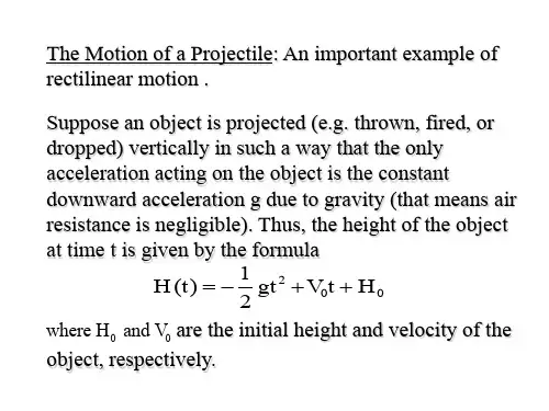
acceleration acting on the object is the constant
downward acceleration g due to gravityistance is negligible). Thus, the height of the object
at time t is given by the formula
H
(t )
1 2
gt 2
V0t
H0
where H0 and V0 are the initial height and velocity of the object, respectively.
Example 10 Suppose a person standing at the top of a building 112 feet high throws a ball vertically upward with an initial velocity of 96 ft/sec.
微积分讲解ppt课件

多元函数的表示 方法
多元函数可用记号 f(x1,x2,…,xn)或z=f(x,y) 表示。
多元函数的定义 域
使多元函数有意义的自 变量组合(x1,x2,…,xn) 的集合。
多元函数的值域
多元函数所有值的集合 。
偏导数与全微分
偏导数的定义
设函数z=f(x,y)在点(x0,y0)的某一邻域内有定义,当y固定在y0而x在x0处有增量Δx时,相应地函数有增量 f(x0+Δx,y0)-f(x0,y0)。如果Δz与Δx之比当Δx→0时的极限存在,那么此极限值称为函数z=f(x,y)在点(x0,y0)处对 x的偏导数。
齐次方程法
通过变量替换,将齐次方程转化为可分离变 量的形式
一阶线性微分方程法
利用积分因子,将方程转化为可积分的形式
二阶常微分方程解法
可降阶的二阶微分方程
通过变量替换或分组,将方程降为一阶微分方 程求解
二阶线性微分方程法
利用特征根的性质,求解二阶线性常系数齐次 和非齐次微分方程
常系数线性微分方程组法
在经济学中的应用
边际分析
通过求导计算边际成本、边际收益等,为企业的决策 提供依据。
弹性分析
研究价格、需求等经济变量之间的相对变化关系,微 积分可用于计算弹性系数。
最优化问题
在资源有限的情况下,通过微积分求解最大化或最小 化某一经济指标的问题。
在工程学中的应用
结构力学
分析建筑、桥梁等结构的受力情况和稳定性,微积分可用 于求解复杂的力学方程。
通过消元法或特征根法,求解常系数线性微分方程组
05
多元函数微积分
多元函数的基本概念
多元函数的定义
设D为一个非空的n元有 序数组的集合,f为某一 确定的对应规则。若对 于每一个有序数组 (x1,x2,…,xn)∈D,通过 对应规则f,都有唯一确 定的实数y与之对应, 则称对应规则f为定义在 D上的n元函数。
微积分一些相关PPT
微分学
微分学主要研究的是在函数自变量变化时如
何确定函数值的瞬时变化率(或微分)。换 言之,计算导数的方法就叫微分学。微分学 的另一个计算方法是牛顿法,该算法又叫应 用几何法,主要通过函数曲线的切线来寻找 点斜率。费马常被称作“微分学的鼻祖”。
积分学
积分学是微分学的逆运算,即从导数推算出
原函数,又分为定积分与不定积分。一个一元 函数的定积分可以定义为无穷多小矩形的面 积和,约等于函数曲线下包含的实际面积。 因此,我们可以用积分来计算平面上一条曲 线所包含的面积、球体或圆锥体的表面积或 体积等。而不定积分的用途较少,主要用于 微分方程的解。
牛顿
牛顿在1671年写了《流数法和 无穷级数》,这本书直到1736 年才出版,它在这本书里指出: 变量是由点、线、面的连续运动产生的,否定了以 前自己认为的变量是无穷小元素的静止集合。他把 连续变量叫做流动量,把这些流动量的导数叫做流 数。牛顿在流数术中所提出的中心问题是:已知连 续运动的路径,求给定时刻的速度(微分法);已 知运动的速度求给定时间内经过的路程(积分法)。
2:微积分的创立
微积分学的建立 从微积分成为一门学科来说,是在十七世纪,但是,微分和 积分的思想在古代就已经产生了。 极限的产生 公元前三世纪,古希腊的阿基米德在研究解决抛物弓形的面 积、球和球冠面积、螺线下面积和旋转双曲体的体积的问题 中,就隐含着近代积分学的思想。作为微分学基础的极限理 论来说,早在古代以有比较清楚的论述。比如中国的庄周所 著的《庄子》一书的“天下篇”中,记有“一尺之棰,日取 其半,万世不竭”。三国时期的刘徽在他的割圆术中提到 “割之弥细,所失弥小,割之又割,以至于不可割,则与圆 周和体而无所失矣。”这些都是朴素的、也是很典型的极限 概念。
托马斯微积分课件8.7 Taylor and Maclaurin Series
Analysis.
1 1 1 n 1 2 f x 2 x 2 3 x 2 n 1 x 2 2 2 2 2 12 1 x2 1 x 0, 4 1 x 2 2 x 2
n
1 n 1 2 n 1
1 1 2 x 1,1 , x , . 2 2
1 n 1 n n n 1 1 n f x x 2 x 1 2 x , x , . 3 n 0 2 2 n 0 3 n 0
目录
上页
下页
返回
结束
Solution. The Taylor series generated by f at 0 is
The Taylor polynomial is
目录
上页
下页
返回
结束
Two questions: 1. How accurately do a function’s Taylor polynomial approximate the function on a given interval?
Step 3. Draw a conclusion.
目录 上页 下页 返回 结束
Example 5.
Solution.
目录
上页
下页
返回
结束
Example 6.
Solution.
目录
上页
下页
返回
结束
Example 7.
Solution.
目录
上页
下页
返回
结束
Example 10.
Solution.
x
托马斯微积分课件8.1 Limits os Sequences of Numbers
Chapter 8 Infinite Series
8.1 Limits of Sequences of Numbers 8.2 Subsequences, Bounded Sequences, and… 8.3 Infinite Series 8.4 Series of Nonnegative Terms 8.5 Alternating Series, Absolute and Conditional Convergence 8.6 Power Series 8.7 Taylor and Maclaurin Series 8.8 Applications of Power Series
n
பைடு நூலகம்
n
n 1 ln n 1
n
e
n ln
n 1 n 1
n 1 n e lim e n n 1 1 lim ln n 1 ln n 1 n e n
n 1 lim nln n n 1
ln n 4 n n 4 lim
1 n 4
e
1 lim ln n 4 n n 4
e
1 n n 4 lim
e
1
0
目录
上页
下页
返回
结束
Example 10. Applying the L’Hospital Rule
Solution.
n 1 e n 1
目录
上页
下页
返回
结束
目录
上页
下页
返回
结束
Example 1. Applying the definition to show that
Solution. We must find the integer N such that for all n
8.1 Limits of Sequences of Numbers 8.2 Subsequences, Bounded Sequences, and… 8.3 Infinite Series 8.4 Series of Nonnegative Terms 8.5 Alternating Series, Absolute and Conditional Convergence 8.6 Power Series 8.7 Taylor and Maclaurin Series 8.8 Applications of Power Series
n
பைடு நூலகம்
n
n 1 ln n 1
n
e
n ln
n 1 n 1
n 1 n e lim e n n 1 1 lim ln n 1 ln n 1 n e n
n 1 lim nln n n 1
ln n 4 n n 4 lim
1 n 4
e
1 lim ln n 4 n n 4
e
1 n n 4 lim
e
1
0
目录
上页
下页
返回
结束
Example 10. Applying the L’Hospital Rule
Solution.
n 1 e n 1
目录
上页
下页
返回
结束
目录
上页
下页
返回
结束
Example 1. Applying the definition to show that
Solution. We must find the integer N such that for all n
微积分英文版课件
Applications of Derivatives
Local Extrema
Discover how derivatives help identify local maximums and minimums of functions.
Mean Value Theorem
Explore the mean value theorem and its applications in calculus.
Gradients and Directional Derivatives
2
derivatives and their applications in multivariable calculus.
Learn about gradients and
directional derivatives for
Derivatives
1
Definition of a Derivative
Uncover the definition and
Differentiability and Continuity
2
fundamental properties of derivatives.
Understand the relationship
Discover the conditions for a function to be continuous and its implications.
Explore the different types of discontinuities and their characteristics.
Conclusion
Review of Key Concepts