递归神经网络英文课件-Chapter 2 Machine learning basics
合集下载
MLP神经网络PPT课件

contents
• structure • universal theorem • MLP for classification • mechanism of MLP for classification
– nonlinear mapping – binary coding of the areas
i, j
Ep i jk
O k1 i
• Situation for k M
E p i jM
E p O j M
O j M i jM
( y j OjM ) f '(ijM )
• Situation for k M
Ep
i jk
l
E p il k1
il k1 O j k
O j k i jk
l
• We ended by looking at some practical issues that didn’t arise for the single layer networks
Structure of an MLP
• it is composed of several layers • neurons within each layer are not connected • ith layer is only fully connected to the (i+1)jth layer • Signal is transmitted only in a feedforward manner
ij (xi )
• It is impractical
– the functions Ej(.) and ij (.) are not the simple weighted sums passed through
神经网络课件2
Computation of actual response
y(n) sgn[ wT (n)x(n)]
Adaptation of Weight Vector
w(n 1) w(n) [d (n) y(n)]x(n)
1 if x(n) belongs to class C1 d ( n) { 1 if x(n) belongs to class C 2 Continuation
Perceptron Convergence Theorem(II)
Using modified signal-flow graph
bias
b(n) is treated as synaptic weight driven by fixed input +1 w0 ( n) is b(n) linear combiner output
m
of bias b is merely to shift decision boundary away from origin synaptic weights adapted on iteration by iteration basis
Perceptron(II)
Decision regions separated by a hyperplane
Perceptron
The simplest form of a neural network consists of a single neuron with adjustable synaptic weights and bias. performs pattern classification with only two classes perceptron convergence theorem :
Machine Learning.ppt

History of ML(1990s & beyond)
What’s hot now? Reinforcement learning; Bayesian learning; automatic bias selection; inductive logic programming (mostly in Europe); applications to robotics; adaptive software agents; voting, bagging, boosting, and stacking.
.. ..
x1
x1+x2+1=0
2x2=0 x1
step 4 input (x1,x2) = (-1,1) , t = -1
ww120211((11))11 b 0 (1) 1
step 5 input (x1,x2) = (-1,-1) , t = -1
w1 1 (1) (1) 2 w2 1 (1) (1) 2 b 1 (1) 2
Machine Learning <T,P,E>:
Computer automatically improves
at task T(任务) according to performance metric P(性能) through experience E(经验)
--- Tom Mitchell
T: Driving on four-lane highways using vision sensors
P: Average distance traveled before a human-judged error
E: A sequence of images and steering commands recorded while observing a human driver.
神经网络学习PPT课件
d ||X1 X 2|| ( X1 X 2 )( X1-X 2 )T
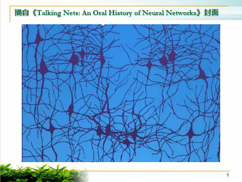
摘自《Talking Nets: An Oral History of Neural Networks》封面
2008-2009学年第1学期
1
神经网络基础
公元前400年左右,柏拉图和亚里士多德就曾对 人类认知、记忆、思维进行过研究;
19世纪末,出现了神经元学说;美国生物学家W. James在《Physiology》一书中提到,“人脑中 两个基本单元靠得较近时,一个单元的兴奋会传 到另一个单元;
2008-2009学年第1学期
16
“感知器”无法解决线性不可分问题;
1969年,Minsky和Papert指出了“感知器”的 这种局限性,例如,“感知器”无法实现“异或”
逻辑。
逻辑“与”
逻辑“异或”
x1
x2
y
x1
x2
y
0
0
0
0
0
0
0
1
0
0
1
1
1
0
0
1
0
1
1
1
1
1
1
0
2008-2009学年第1学期
输入一个实际例子,让ANN分析并给出结果。
2008-2009学年第1学期
12
“感知器”是怎么训练的呢?
假设每个样本含 n 个属性,用向量(x1, x2, …, xn)表示;若 X 为样本变量, X∈Rn;
wij 是 xi 到神经元 j 的连接权值, Wj 是神经元 j 的输入连 接的权值向量,即Wj =(w1j , w2j , …, wnj );
第i层神经元netij层神经元的数目20082009学年第1学神经网络学习bp算法中的前向计算ijijnetijij特征函数必须是有界连续可微的如sigmoid函数20082009学年第1学期神经网络学习bp算法中的反向计算ijkijkijkijkijk输出层神经元j的状态误差ijk的调整量20082009学年第1学期神经网络学习bp算法中的反向计算续ikik神经网络学习bp学习算法的特点对于n层网络结构学习后可得到n1个超曲面组成复合曲面从而实现复杂的分类任务
《ANN神经网络》课件

神经网络的训练过程和算法
1 BP算法
2 Adam算法
通过反向传播算法,根据输出误差和梯度下 降法更新网络参数,目标是最小化误差函数。
结合了Ad ag r ad 和RM Sp ro p 优点的一种有效 的优化算法,自适应的调节学习率,以加快 训练速度。
神经网络的激活函数和正则化方法
激活函数
每个神经元的输出需要通过激活函数进行非线性映 射,目前比较流行的有sig mo id 、t an h 和ReLU等。
神经元和生物神经元的异同
1 神经元
是神经网络的基本单位,是一种用于计算的抽象模型,只有输入和输出,以及需要学习 的权重和偏置。
2 生物神经元
是神经系统的基本单位,由轴突、树突、细胞体和突触等结构组成,与其他神经元具有 复杂的生物学表现和相互作用。
神经网络的优势和局限性
优势
具有自主学习、自适应、非线性和可并行处理等优 势,能够处理高维度数据和复杂的非线性问题。
参考文献和拓展阅读建议
参考文献: 1. Bishop, C. M . (1995). Neural Networks for Pattern Recognition. Oxford University Press. 2. Goodfellow, I., Bengio, Y., & Courville, A. (2016). Deep Learning. M IT Press. 3. LeCun, Y., Bengio, Y., & Hinton, G. (2015). Deep Learning. Nature, 521, 436-444. 拓展阅读建议: 1. 《深度学习》白板推导与Python实战 2. 《Python深度学习》实践指南 3. 《自然语言处理综论》 4. 《计算机视觉综论》
NEURALNETWORKS培训课件.ppt

components are independent of each other.
Introduction
Biological neural networks are much more complicated in their elementary structures than the mathematical models we use for ANNs.
techniques A neural network is a processing device, either an algorithm, or actual hardware, whose
design was motivated by the design and functioning of human brains and components thereof. Most neural networks have some sort of "training" rule whereby the weights of connections
The Brain
The Brain as an Information Processing System The human brain contains about 10 billion nerve cells, or neurons. On average, each neuron is connected to other neurons through about 10 000 synapses. (The actual figures vary greatly, depending on the local neuroanatomy.)
Neural networks are a powerful technique to solve many real world problems. They have the ability to learn from experience in order to improve their performance and to adapt themselves to changes in the environment. In addition to that they are able to deal with incomplete information or noisy data and can be very effective especially in situations where it is not possible to define the rules or steps that lead to the solution of a problem.
神经网络
α1 α2 α3 α4 . . . αT
T
αt sign wtT x
gt (x)
G
G(x) = sign
t =1
• two layers of weights:
wt and α
• two layers of sign functions:
in gt and in G
what boundary can G implement?
−
−
+ + + +
−
−
+ + + +
−
−
−
−
−
−
−
8 perceptrons
16 perceptrons
target boundary
• ‘convex set’ hypotheses implemented: dVC → ∞, remember? :-) • powerfulness: enough perceptrons ≈ smooth boundary
linear regression
h(x) = s
x0 x1 x2 xd s h(x)
logistic regression
h(x) = θ(s)
x0 x1 x2 xd s h(x)
err = 0/1
err = squared
err = cross-entropy
will discuss ‘regression’ with squared error
2
G(x) = sign
t =0 1 2 3 4
αt gt (x)
to implement OR(g1 , g2 )?
神经网络ppt课件

神经元层次模型 组合式模型 网络层次模型 神经系统层次模型 智能型模型
通常,人们较多地考虑神经网络的互连结构。本 节将按照神经网络连接模式,对神经网络的几种 典型结构分别进行介绍
12
2.2.1 单层感知器网络
单层感知器是最早使用的,也是最简单的神经 网络结构,由一个或多个线性阈值单元组成
这种神经网络的输入层不仅 接受外界的输入信号,同时 接受网络自身的输出信号。 输出反馈信号可以是原始输 出信号,也可以是经过转化 的输出信号;可以是本时刻 的输出信号,也可以是经过 一定延迟的输出信号
此种网络经常用于系统控制、 实时信号处理等需要根据系 统当前状态进行调节的场合
x1
…… …… ……
…… yi …… …… …… …… xi
再励学习
再励学习是介于上述两者之间的一种学习方法
19
2.3.2 学习规则
Hebb学习规则
这个规则是由Donald Hebb在1949年提出的 他的基本规则可以简单归纳为:如果处理单元从另一个处
理单元接受到一个输入,并且如果两个单元都处于高度活 动状态,这时两单元间的连接权重就要被加强 Hebb学习规则是一种没有指导的学习方法,它只根据神经 元连接间的激活水平改变权重,因此这种方法又称为相关 学习或并联学习
9
2.1.2 研究进展
重要学术会议
International Joint Conference on Neural Networks
IEEE International Conference on Systems, Man, and Cybernetics
World Congress on Computational Intelligence
复兴发展时期 1980s至1990s
- 1、下载文档前请自行甄别文档内容的完整性,平台不提供额外的编辑、内容补充、找答案等附加服务。
- 2、"仅部分预览"的文档,不可在线预览部分如存在完整性等问题,可反馈申请退款(可完整预览的文档不适用该条件!)。
- 3、如文档侵犯您的权益,请联系客服反馈,我们会尽快为您处理(人工客服工作时间:9:00-18:30)。
Xiaogang Wang
Machine Lzation
We care more about the performance of the model on new, previously unseen examples
The training examples usually cannot cover all the possible input configurations, so the learner has to generalize from the training examples to new cases
y ∗ = arg max P(y = k |x)
k
(Duda et al. Pattern Classification 2000) Xiaogang Wang
Machine Learning Basics
cuhk
Regression
Predict real-valued output f : RD → RM
Mean squared error (MSE) for linear regression
MSEtrain
=
1 N
||wt x(itrain) − yi(train)||22
i
Cross entropy (CE) for classification
CEtrain
=
1 N
log P(y = yi(train)|x(itrain))
wMSEtrain = 0 ⇒ w||X(train)w − y(train)||22 = 0 w = (X(train)t X(train))−1X(train)t y(train) where X(train) = [x(1train), . . . , x(Ntrain)] and y(train) = [y1(train), . . . , yN(train)].
1 Performancetest = M
M
Error(f (x(i test)), yi(test))
i =1
We hope that both test examples and training examples are drawn from p(x, y ) of interest, although it is unknown
i
Why not use classification errors #{f (x(itrain)) = yi(train)}?
cuhk
Xiaogang Wang
Machine Learning Basics
Optimization
The choice of the objective function should be good for optimization Take linear regression as an example
GEf = p(x, y )Error(f (x), y )
x,y
cuhk
Xiaogang Wang
Machine Learning Basics
Generalization
However, in practice, p(x, y ) is unknow. We assess the generalization performance with a test set {x(i test), yi(test)}
Decision boundary, parameters of P(y |x), and w in linear regression
Optimize an objective function on the training set. It is a performance measure on the training set and could be different from that on the test set.
Generalization error: the expected error over ALL examples
To obtain theoretical guarantees about generalization of a machine learning algorithm, we assume all the samples are drawn from a distribution p(x, y ), and calculate generalization error (GE) of a prediction function f by taking expectation over p(x, y )
f (x) is decided by the decision boundary As an variant, f can also predict the probability distribution over classes given x, f (x) = P(y |x). The category is predicted as
Machine Learning Basics
Xiaogang Wang
Machine Learning Basics
cuhk
Machine Learning
Xiaogang Wang
Machine Learning Basics
cuhk
Classification
f (x) predicts the category that x belongs to f : RD → {1, . . . , K }
Example: linear regression
D
y = wt x = wd xd + w0
d =1
(Bengio et al. Deep Learning 2014)
Xiaogang Wang
Machine Learning Basics
cuhk
Training
Training: estimate the parameters of f from {(x(itrain), yi(train))}