投资学模拟试题第六套
投资学课后习题与答案(博迪)_第6版

投资学习题第一篇投资学课后习题与答案乮博迪乯_第6版 由flyesun 从网络下载丆版权归原作者所有。
1. 假设你发现一只装有1 00亿美元的宝箱。
a. 这是实物资产还是金融资产?b. 社会财富会因此而增加吗?c. 你会更富有吗?d. 你能解释你回答b 、c 时的矛盾吗?有没有人因为这个发现而受损呢?2. Lanni Products 是一家新兴的计算机软件开发公司,它现有计算机设备价值30 000美元,以及由L a n n i 的所有者提供的20 000美元现金。
在下面的交易中,指明交易涉及的实物资产或(和)金融资产。
在交易过程中有金融资产的产生或损失吗?a. Lanni 公司向银行贷款。
它共获得50 000美元的现金,并且签发了一张票据保证3年内还款。
b. Lanni 公司使用这笔现金和它自有的20 000美元为其一新的财务计划软件开发提供融资。
c. L a n n i 公司将此软件产品卖给微软公司( M i c r o s o f t ),微软以它的品牌供应给公众,L a n n i 公司获得微软的股票1 500股作为报酬。
d. Lanni 公司以每股80美元的价格卖出微软的股票,并用所获部分资金偿还贷款。
3. 重新考虑第2题中的Lanni Products 公司。
a. 在它刚获得贷款时处理其资产负债表,它的实物资产占总资产的比率为多少?b. 在L a n n i 用70 000美元开发新产品后,处理资产负债表,实物资产占总资产比例又是多少?c. 在收到微软股票后的资产负债表中,实物资产占总资产的比例是多少?4. 检察金融机构的资产负债表,有形资产占总资产的比率为多少?对非金融公司这一比率又如何?为什么会有这样的差异?5. 20世纪6 0年代,美国政府对海外投资者所获得的在美国出售的债券的利息征收 3 0%预扣税(这项税收现已被取消),这项措施和与此同时欧洲债券市场(美国公司在海外发行以美元计值的债券的市场)的成长有何关系?6. 见图1 -7,它显示了美国黄金证券的发行。
投资学习题及答案6.16
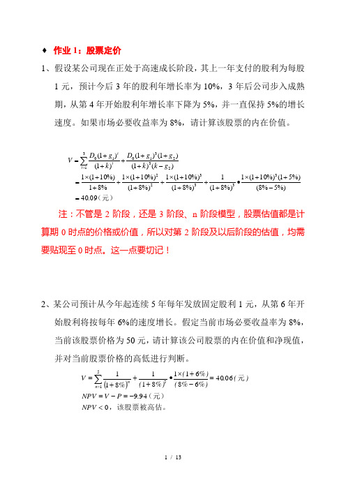
♦ 作业1:股票定价1、假设某公司现在正处于高速成长阶段,其上一年支付的股利为每股1元,预计今后3年的股利年增长率为10%,3年后公司步入成熟期,从第4年开始股利年增长率下降为5%,并一直保持5%的增长速度。
如果市场必要收益率为8%,请计算该股票的内在价值。
(元) 09.40%)5%8(%)51(%)101(1%)81(1%)81(%)101(1%)81(%)101(1%81%)101(1)()1()1()1()1()1(3333222323103110=-++⨯•++++⨯+++⨯+++⨯=-++++++=∑=g k k g g D k g D V t tt 注:不管是2阶段,还是3阶段、n 阶段模型,股票估值都是计算期0时点的价格或价值,所以对第2阶段及以后阶段的估值,均需要贴现至0时点。
这一点要切记!2、某公司预计从今年起连续5年每年发放固定股利1元,从第6年开始股利将按每年6%的速度增长。
假定当前市场必要收益率为8%,当前该股票价格为50元,请计算该公司股票的内在价值和净现值,并对当前股票价格的高低进行判断。
(),该股票被高估。
(元)元0949064068611811811551<-=-==-+⨯•+++=∑=NPV .P V NPV )(.%)%(%)(%)(%V n n3、某股份公司去年支付每股股利1元,预计在未来该公司股票股利按每年6%的速率增长,假定必要收益率为8%,请计算该公司股票的内在价值。
当前该股票价格为30元,请分别用净现值法和内部收益率法判断该股票的投资价值。
(1)净现值法:)(%%%)(V 元5368611=-+⨯=。
低估,建议购买该股票,所以当前股票价格被023>=-=P V NPV(2)内部收益率法:30=%6%)61(1-+⨯r , r =9.5%>8%(必要收益率)当前股票价格被低估,建议购买该股票。
4、某上市公司上年每股股利为0.3元,预计以后股利每年以3%的速度递增。
投资学6单元题目及答案

Problem3: Draw the indifference curve in the expected return–standard deviation plane corresponding to a utility level of 5% for an investor with a risk aversion coefficient of 3. (Hint: Choose several possible standard deviations, ranging from 5% to 25%, and find the expected rates of return providing a utility level of 5%. Then plot the expected return–standard deviation points so derived. answers: Points on the curve are derived by solving for E(r) in the following equation: U = 5 = E(r) – 0.005A = E(r) – 0.015 E(r) =U+ 0.015
Problem5(*): Based on the utility formula above, which investment would you select if you were risk neutral? a. 1. b. 2. c. 3. d. 4. answers: d [When investors are risk neutral, then A = 0; the portfolio with the highest utility is the one with the highest expected return.] Problem6(*): The variable (A) in the utility formula represents the: a. investor’s return requirement. b. investor’s aversion to risk. c. certainty equivalent rate of the portfolio. d. preference for one unit of return per four units of risk. answers: b Consider historical data showing that the average annual rate of return on the S&P 500 portfolio over the past 70 years has averaged about 8.5% more than the Treasury bill return and that the S&P 500 standard deviation has been about 20% per year. Assume these values are representative of investors’ expectations for future performance and that the current T-bill rate is 5%. Use these values to solve problems 7 to 8. Problem7: Calculate the expected return and variance of portfolios invested in T-bills and the S&P500 index with weights as follows:
投资学第10版习题答案06分析解析

CHAPTER 6: CAPITAL ALLOCATION TO RISKY ASSETS PROBLEM SETS1. (e) The first two answer choices are incorrect because a highly risk averse investorwould avoid portfolios with higher risk premiums and higher standard deviations.In addition, higher or lower Sharpe ratios are not an indication of an investor'stolerance for risk. The Sharpe ratio is simply a tool to absolutely measure the return premium earned per unit of risk.2. (b) A higher borrowing rate is a consequence of the risk of the borr owers’ default.In perfect markets with no additional cost of default, this increment would equal the value of the borrower’s option to default, and the Sharpe measure, with appropriate treatment of the default option, would be the same. However, in reality there arecosts to default so that this part of the increment lowers the Sharpe ratio. Also,notice that answer (c) is not correct because doubling the expected return with afixed risk-free rate will more than double the risk premium and the Sharpe ratio. 3. Assuming no change in risk tolerance, that is, an unchanged risk-aversioncoefficient (A), higher perceived volatility increases the denominator of theequation for the optimal investment in the risky portfolio (Equation 6.7). Theproportion invested in the risky portfolio will therefore decrease.4. a. The expected cash flow is: (0.5 × $70,000) + (0.5 × 200,000) = $135,000.With a risk premium of 8% over the risk-free rate of 6%, the required rate ofreturn is 14%. Therefore, the present value of the portfolio is:$135,000/1.14 = $118,421b. If the portfolio is purchased for $118,421 and provides an expected cashinflow of $135,000, then the expected rate of return [E(r)] is as follows:$118,421 × [1 + E(r)] = $135,000Therefore, E(r) =14%. The portfolio price is set to equate the expected rate ofreturn with the required rate of return.c. If the risk premium over T-bills is now 12%, then the required return is:6% + 12% = 18%The present value of the portfolio is now:$135,000/1.18 = $114,407d. For a given expected cash flow, portfolios that command greater riskpremiums must sell at lower prices. The extra discount from expectedvalue is a penalty for risk.5.When we specify utility by U = E(r) – 0.5Aσ2, the utility level for T-bills is: 0.07The utility level for the risky portfolio is:U = 0.12 – 0.5 ×A × (0.18)2 = 0.12 – 0.0162 ×AIn order for the risky portfolio to be preferred to bills, the following must hold:0.12 – 0.0162A > 0.07 ⇒A < 0.05/0.0162 = 3.09A must be less than 3.09 for the risky portfolio to be preferred to bills.6. Points on the curve are derived by solving for E(r) in the following equation:U = 0.05 = E(r) – 0.5Aσ2 = E(r) – 1.5σ2The values of E(r), given the values of σ2, are therefore:σσ 2E(r)0.00 0.0000 0.050000.05 0.0025 0.053750.10 0.0100 0.065000.15 0.0225 0.083750.20 0.0400 0.110000.25 0.0625 0.14375The bold line in the graph on the next page (labeled Q6, for Question 6) depicts the indifference curve.7. Repeating the analysis in Problem 6, utility is now:U = E(r) – 0.5Aσ2 = E(r) –2.0σ2 = 0.05The equal-utility combinations of expected return and standard deviation arepresented in the table below. The indifference curve is the upward sloping line in the graph on the next page, labeled Q7 (for Question 7).σσ 2E(r)0.00 0.0000 0.05000.05 0.0025 0.05500.10 0.0100 0.07000.15 0.0225 0.09500.20 0.0400 0.13000.25 0.0625 0.1750The indifference curve in Problem 7 differs from that in Problem 6 in slope.When A increases from 3 to 4, the increased risk aversion results in a greaterslope for the indifference curve since more expected return is needed in order to compensate for add itional σ.8. The coefficient of risk aversion for a risk neutral investor is zero. Therefore, thecorresponding utility is equal to the portfolio’s expected return. The corresponding indifference curve in the expected return-standard deviation plane is a horizontal line, labeled Q8 in the graph above (see Problem 6).9. A risk lover, rather than penalizing portfolio utility to account for risk, derivesgreater utility as variance increases. This amounts to a negative coefficient of risk aversion. The corresponding indifference curve is downward sloping in the graph above (see Problem 6), and is labeled Q9.10. The portfolio expected return and variance are computed as follows:(1) W Bills (2)r Bills(3)W Index(4)r Indexr Portfolio(1)×(2)+(3)×(4)σPortfolio(3) × 20%σ 2 Portfolio0.0 5% 1.0 13.0% 13.0% = 0.130 20% = 0.20 0.04000.2 5 0.8 13.0 11.4% = 0.114 16% = 0.16 0.02560.4 5 0.6 13.0 9.8% = 0.098 12% = 0.12 0.01440.6 5 0.4 13.0 8.2% = 0.082 8% = 0.08 0.00640.8 5 0.2 13.0 6.6% = 0.066 4% = 0.04 0.00161.0 5 0.0 13.0 5.0% = 0.050 0% = 0.00 0.0000 11. Computing utility from U = E(r) – 0.5 ×Aσ2 = E(r) –σ2, we arrive at the values inthe column labeled U(A = 2) in the following table:W Bills W Index r PortfolioσPortfolioσ2Portfolio U(A = 2) U(A = 3)0.0 1.0 0.130 0.20 0.0400 0.0900 .07000.2 0.8 0.114 0.16 0.0256 0.0884 .07560.4 0.6 0.098 0.12 0.0144 0.0836 .07640.6 0.4 0.082 0.08 0.0064 0.0756 .07240.8 0.2 0.066 0.04 0.0016 0.0644 .06361.0 0.0 0.050 0.00 0.0000 0.0500 .0500The column labeled U(A = 2) implies that investors with A = 2 prefer a portfolio that is invested 100% in the market index to any of the other portfolios in the table.12. The column labeled U(A = 3) in the table above is computed from:U = E(r) – 0.5Aσ2 = E(r) – 1.5σ2The more risk averse investors prefer the portfolio that is invested 40% in themarket, rather than the 100% market weight preferred by investors with A = 2.13. Expected return = (0.7 × 18%) + (0.3 × 8%) = 15%Standard deviation = 0.7 × 28% = 19.6%14. Investment proportions: 30.0% in T-bills0.7 × 25% = 17.5% in Stock A0.7 × 32% = 22.4% in Stock B0.7 × 43% = 30.1% in Stock C15. Your reward-to-volatility ratio:.18.080.3571.28S-==Client's reward-to-volatility ratio:.15.080.3571.196S-==16.17. a. E(r C) = r f + y × [E(r P) –r f] = 8 + y × (18 - 8)If the expected return for the portfolio is 16%, then:16% = 8% + 10% ×y⇒.16.080.8.10y-==Therefore, in order to have a portfolio with expected rate of return equal to 16%, the client must invest 80% of total funds in the risky portfolio and 20% in T-bills.b.Client’s investment proportions:20.0% in T-bills0.8 × 25% = 20.0% in Stock A0.8 × 32% = 25.6% in Stock B0.8 × 43% = 34.4% in Stock Cc. σC = 0.8 ×σP = 0.8 × 28% = 22.4%18. a.σC = y × 28%If your client prefers a standard deviation of at most 18%, then: y = 18/28 = 0.6429 = 64.29% invested in the risky portfolio.b. ().08.1.08(0.6429.1)14.429%C E r y =+⨯=+⨯=19. a.y *0.36440.27440.100.283.50.080.18σ22==⨯-=-=PfP A r )E(rTherefo re, the client’s optimal proportions are: 36.44% invested in the risky portfolio and 63.56% invested in T-bills.b. E (r C ) = 0.08 + 0.10 × y * = 0.08 + (0.3644 × 0.1) = 0.1164 or 11.644% σC = 0.3644 × 28 = 10.203%20. a.If the period 1926–2012 is assumed to be representative of future expected performance, then we use the following data to compute the fraction allocated to equity: A = 4, E (r M ) − r f = 8.10%, σM = 20.48% (we use the standard deviation of the risk premium from Table 6.7). Then y * is given by:That is, 48.28% of the portfolio should be allocated to equity and 51.72% should be allocated to T-bills.b.If the period 1968–1988 is assumed to be representative of future expected performance, then we use the following data to compute the fraction allocated to equity: A = 4, E (r M ) − r f = 3.44%, σM = 16.71% and y * is given by:22()0.0344*0.308040.1671M fME r r y A σ-===⨯Therefore, 30.80% of the complete portfolio should be allocated to equity and 69.20% should be allocated to T-bills.c.In part (b), the market risk premium is expected to be lower than in part (a) and market risk is higher. Therefore, the reward-to-volatility ratio is expected to be lower in part (b), which explains the greater proportion invested in T-bills.21. a. E (r C ) = 8% = 5% + y × (11% – 5%) ⇒ .08.050.5.11.05y -==-b. σC = y × σP = 0.50 × 15% = 7.5%c.The first client is more risk averse, preferring investments that have less risk as evidenced by the lower standard deviation.22. Johnson requests the portfolio standard deviation to equal one half the marketportfolio standard deviation. The market portfolio 20%M σ=, which implies10%P σ=. The intercept of the CML equals 0.05f r =and the slope of the CMLequals the Sharpe ratio for the market portfolio (35%). Therefore using the CML:()()0.050.350.100.0858.5%M fP f P ME r r E r r σσ-=+=+⨯==23. Data: r f = 5%, E (r M ) = 13%, σM = 25%, and B f r = 9%The CML and indifference curves are as follows:24. For y to be less than 1.0 (that the investor is a lender), risk aversion (A ) must belarge enough such that:1σ<-=2M fM A r )E(r y ⇒ 1.280.250.050.132=->A For y to be greater than 1 (the investor is a borrower), A must be small enough:1σ)(>-=2MfM A r r E y ⇒ 0.640.250.090.132=-<AFor values of risk aversion within this range, the client will neither borrow nor lend but will hold a portfolio composed only of the optimal risky portfolio:y = 1 for 0.64 ≤ A ≤ 1.2825. a.The graph for Problem 23 has to be redrawn here, with: E (r P ) = 11% and σP = 15%b. For a lending position: 2.670.150.050.112=->AFor a borrowing position: 0.890.150.090.112=-<A Therefore, y = 1 for 0.89 ≤ A ≤ 2.6726. The maximum feasible fee, denoted f , depends on the reward-to-variability ratio.For y < 1, the lending rate, 5%, is viewed as the relevant risk-free rate, and we solve for f as follows:.11.05.13.05.15.25f ---= ⇒ .15.08.06.012, or 1.2%.25f ⨯=-= For y > 1, the borrowing rate, 9%, is the relevant risk-free rate. Then we notice that,even without a fee, the active fund is inferior to the passive fund because:.11 – .09 – f= 0.13 <.13 – .09= 0.16 → f = –.004.15 .25More risk tolerant investors (who are more inclined to borrow) will not be clients of the fund. We find that f is negative: that is, you would need to pay investors to choose your active fund. These investors desire higher risk –higher return completeportfolios and thus are in the borrowing range of the relevant CAL. In this range, the reward-to-variability ratio of the index (the passive fund) is better than that of the managed fund. 27. a.Slope of the CML .13.080.20-==28. a.With 70% of hi s money invested in my fund’s portfolio, the client’s expected return is 15% per year with a standard deviation of 19.6% per year. If he shifts that money to the passive portfolio (which has an expected return of 13% and standard deviation of 25%), his overall expected return becomes: E (r C ) = r f + 0.7 × [E (r M ) − r f ] = .08 + [0.7 × (.13 – .08)] = .115, or 11.5% The standard deviation of the complete portfolio using the passive portfolio would be:σC = 0.7 × σM = 0.7 × 25% = 17.5%Therefore, the shift entails a decrease in mean from 15% to 11.5% and a decrease in standard deviation from 19.6% to 17.5%. Since both mean return and standard deviation decrease, it is not yet clear whether the move is beneficial. The disadvantage of the shift is that, if the client is willing to accept a mean return on his total portfolio of 11.5%, he can achieve it with a lower standard deviation using my fund rather than the passive portfolio. To achieve a target mean of 11.5%, we first write the mean of the completeportfolio as a function of the proportion invested in my fund (y ):E (r C ) = .08 + y × (.18 − .08) = .08 + .10 × yOur target is: E (r C ) = 11.5%. Therefore, the proportion that must be invested in my fund is determined as follows:.115 = .08 + .10 × y ⇒ .115.080.35.10y -== The standard deviation of this portfolio would be:σC = y × 28% = 0.35 × 28% = 9.8%Thus, by using my portfolio, the same 11.5% expected return can be achieved with a standard deviation of only 9.8% as opposed to the standard deviation of 17.5% using the passive portfolio.b.The fee would reduce the reward-to-volatility ratio, i.e., the slope of the CAL. The client will be indifferent between my fund and the passive portfolio if the slope of the after-fee CAL and the CML are equal. Let f denote the fee:Slope of CAL with fee .18.08.10.28.28f f---==Slope of CML (which requires no fee).13.080.20.25-== Setting these slopes equal we have:.100.200.044 4.4%.28ff -=⇒==per year29. a.The formula for the optimal proportion to invest in the passive portfolio is:2σ)(*MfM A r r E y -=Substitute the following: E (r M ) = 13%; r f = 8%; σM = 25%; A = 3.5:20.130.08*0.2286, or 22.86% in the passive portfolio 3.50.25y -==⨯b. The answer here is the same as the answer to Problem 28(b). The fee that youcan charge a client is the same regardless of the asset allocation mix of theclient’s portfolio. You can charge a fee that will equate the reward-to-volatilityratio of your portfolio to that of your competition.CFA PROBLEMS1. Utility for each investment = E(r) – 0.5 × 4 ×σ2We choose the investment with the highest utility value, Investment 3.Investment ExpectedreturnE(r)StandarddeviationσUtilityU1 0.12 0.30 -0.06002 0.15 0.50 -0.35003 0.21 0.16 0.15884 0.24 0.21 0.15182. When investors are risk neutral, then A = 0; the investment with the highest utility isInvestment 4 because it has the highest expected return.3. (b)4. Indifference curve 2 because it is tangent to the CAL.5. Point E6. (0.6 × $50,000) + [0.4 × (-$30,000)] - $5,000 = $13,0007. (b) Higher borrowing rates will reduce the total return to the portfolio and thisresults in a part of the line that has a lower slope.8. Expected return for equity fund = T-bill rate + Risk premium = 6% + 10% = 16%Expected rate of return of the client’s portfolio = (0.6 × 16%) + (0.4 × 6%) = 12% Expected return of the client’s portfolio = 0.12 × $100,000 = $12,000(which implies expected total wealth at the end of the period = $112,000)Standard deviation of client’s overall portfolio = 0.6 × 14% = 8.4%9. Reward-to-volatility ratio = .100.71 .14=CHAPTER 6: APPENDIX1.By year-end, the $50,000 investment will grow to: $50,000 × 1.06 = $53,000Without insurance, the probability distribution of end-of-year wealth is:Probability WealthNo fire 0.999 $253,000Fire 0.001 53,000For this distribution, expected utility is computed as follows:E[U(W)] = [0.999 ×ln(253,000)] + [0.001 ×ln(53,000)] = 12.439582 The certainty equivalent is:W CE = e 12.439582 = $252,604.85With fire insurance, at a cost of $P, the investment in the risk-free asset is: $(50,000 –P)Year-end wealth will be certain (since you are fully insured) and equal to: [$(50,000 –P) × 1.06] + $200,000Solve for P in the following equation:[$(50,000 –P) × 1.06] + $200,000 = $252,604.85 ⇒P = $372.78 This is the most you are willing to pay for insurance. Note that the expected loss is “only” $200, so you are willing to pay a substantial risk premium over the expected value of losses. The primary reason is that the value of the house is a largeproportion of your wealth.2. a. With insurance coverage for one-half the value of the house, the premiumis $100, and the investment in the safe asset is $49,900. By year-end, theinvestment of $49,900 will grow to: $49,900 × 1.06 = $52,894If there is a fire, your insurance proceeds will be $100,000, and theprobability distribution of end-of-year wealth is:Probability WealthNo fire 0.999 $252,894Fire 0.001 152,894For this distribution, expected utility is computed as follows:E[U(W)] = [0.999 ×ln(252,894)] + [0.001×ln(152,894)] = 12.4402225 The certainty equivalent is:W CE = e 12.4402225 = $252,766.77b.With insurance coverage for the full value of the house, costing $200, end-of-year wealth is certain, and equal to:[($50,000 – $200) × 1.06] + $200,000 = $252,788Since wealth is certain, this is also the certainty equivalent wealth of the fully insured position.c.With insurance coverage for 1½ times the value of the house, the premiumis $300, and the insurance pays off $300,000 in the event of a fire. Theinvestment in the safe asset is $49,700. By year-end, the investment of$49,700 will grow to: $49,700 × 1.06 = $52,682The probability distribution of end-of-year wealth is:Probability WealthNo fire 0.999 $252,682Fire 0.001 352,682For this distribution, expected utility is computed as follows:E[U(W)] = [0.999 ×ln(252,682)] + [0.001 ×ln(352,682)] = 12.4402205 The certainty equivalent is:W CE = e 12.440222 = $252,766.27Therefore, full insurance dominates both over- and underinsurance.Overinsuring creates a gamble (you actually gain when the house burns down).Risk is minimized when you insure exactly the value of the house.。
投资学考试试题及答案

投资学考试试题及答案投资学考试试题及答案投资学是金融学中的一个重要分支,研究的是投资决策和资本配置的理论和方法。
在金融行业中,投资学的知识是非常重要的,因为它涉及到投资者如何进行投资决策,如何评估投资项目的风险和回报,以及如何优化资本配置等问题。
在投资学的学习过程中,考试是一种常见的评估方式,下面我们将介绍一些投资学考试的试题及答案。
第一部分:选择题1. 以下哪个是投资学的核心概念?a) 股票b) 风险c) 利率d) 债券答案:b) 风险2. 投资组合是指投资者持有的一组投资资产,以下哪个是投资组合的主要目标?a) 最大化回报b) 最小化风险c) 最大化流动性d) 最小化成本答案:b) 最小化风险3. 市场有效假设是投资学的重要理论之一,以下哪个描述最符合市场有效假设?a) 市场上的价格是随机波动的,无法预测b) 市场上的价格是由供求关系决定的c) 市场上的价格是由投资者的心理预期决定的d) 市场上的价格是由政府的干预决定的答案:a) 市场上的价格是随机波动的,无法预测第二部分:简答题1. 请简要介绍一下投资组合理论。
答案:投资组合理论是投资学的核心理论之一,它研究的是如何选择和构建一个投资组合,以实现最佳的风险回报平衡。
投资组合理论的基本原理是通过将不同的资产进行组合,可以降低整体投资组合的风险,同时提高回报。
投资组合理论的关键是通过投资资产之间的相关性来实现风险的分散,即通过将不同类型的资产组合在一起,可以降低整体投资组合的波动性。
2. 什么是资本资产定价模型(CAPM)?答案:资本资产定价模型(CAPM)是投资学中的一种重要模型,用于估计资产的预期回报率。
CAPM模型的基本原理是资产的预期回报率应该与其风险相关,即高风险资产应该有高回报率,低风险资产应该有低回报率。
CAPM模型的关键是通过计算资产的贝塔系数来衡量其风险,贝塔系数越高,代表资产的风险越大,预期回报率也应该越高。
第三部分:计算题1. 假设有两个投资项目A和B,其预期回报率和风险如下表所示:项目预期回报率风险(标准差)A 10% 15%B 8% 10%请计算项目A和B的夏普比率,并分析哪个项目更具吸引力。
投资学第10版习题答案06
Chapter 6 - Capital Allocation to Risky Assets 6-1 Copyright © 2014 McGraw-Hill Education. All rights reserved. No reproduction or distribution without the prior written consent of McGraw-Hill Education.
CHAPTER 6: CAPITAL ALLOCATION TO RISKY ASSETS PROBLEM SETS
1. (e) The first two answer choices are incorrect because a highly risk averse investor would avoid portfolios with higher risk premiums and higher standard deviations. In addition, higher or lower Sharpe ratios are not an indication of an investor's tolerance for risk. The Sharpe ratio is simply a tool to absolutely measure the return premium earned per unit of risk.
2. (b) A higher borrowing rate is a consequence of the risk of the borrowers’ default. In perfect markets with no additional cost of default, this increment would equal the value of the borrower’s option to default, and the Sharpe measure, with appropriate treatment of the default option, would be the same. However, in reality there are costs to default so that this part of the increment lowers the Sharpe ratio. Also, notice that answer (c) is not correct because doubling the expected return with a fixed risk-free rate will more than double the risk premium and the Sharpe ratio.
投资学第6章参考答案
第6章参考答案1.有效市场的条件:假设条件(1)完全竞争市场;(2)理性投资者主导市场;(3)信息发布渠道畅通;(4)交易无费用,市场不存在摩擦;(5)资金可以在资本市场中自由流动。
充分条件(1)股票市场没有交易成本;(2)所有投资者无成本的平等的获得所有可获得的信息;(3)所有投资者对当前价格和未来价格的变化趋势认识相同,即同质预期。
必要条件(1)股票价格随机游走(random walk);(2)不可能存在持续获得超额利润的交易规则(扣除风险因素);(3)价格迅速准确反映信息;(4)一般投资者和专业投资者的投资业绩无显著差别。
2.有效市场及有效市场假说:有效市场的含义:对于有效市场的内涵,法玛在其论文中进行了明确定义。
他指出,如果市场上存在大量理性的利润最大化投资者,他们每个人都积极地预测每只有价证券的未来价值,通过激烈的竞争,市场达到均衡时的结果是关于每一只证券的过去信息以及到目前时点为止的可以预期到的事件都已经反映在现时的证券价格中。
这样的市场就是有效市场。
有效市场假说:1965年,法玛在《商业期刊》(Journal of Business)上发表的论文,提出了著名的有效市场假说(Efficient Market Hypothesis,EMH)。
该假说认为,在一个充满信息交流和信息竞争的社会里,一个特定的信息能够在证券市场上迅速被投资者知晓,随后,股票市场的竞争将会驱使证券价格充分且及时反映该组信息,从而使得投资者根据该组信息所进行的交易不存在非正常报酬,而只能赚取风险调整的平均市场报酬率。
3.根据信息集的不同,有效市场可以分为三种形式:弱式有效(weak-form market efficiency)。
如果一个市场是弱式有效的,那么该市场的股票价格反映了一切可以从过去的市场交易数据中获得的信息,例如过去的成交价格和成交量等。
弱式有效假说正是著名的随机游走理论。
半强式有效(semi-strong form market efficiency)。
6投资学第六章习题答案
1.噪声交易风险,是指短期内,噪声交易者的交易行为会导致价格在回复均值之前,会进一步偏离资产的真实价值,从而给投资期限较短的套利者带来风险。
它由套利者承担,而且将会限制套利者的套利意愿。
2.P169页
3.P168页“经济解释”
4.P170页
5.
6.“价格泡沫”,是指由于噪声交易者追涨杀跌的心理,价格在没有新信息出现的情况下不断上涨。
噪声交易者采用上述行为模式被称为正反馈投资策略。
7.P177
套利者知道利好消息时,他们意识到当天价格上涨会促使正反馈交易者第二天买入。
考虑到这一点,套利者会选择当天大量买入,促使当天的价格上升并将利好消息完全消化。
第二天,尽管套利者出售证券,而正反馈交易者买入行为仍使价格高于基本水平。
这种价格上升源于套利者预期性的交易行为和正反馈交易者行为的反应。
投资学模拟试卷
厦门大学网络教育2010-2011学年第二学期《投资学》复习题一、单项选择题1、其他条件不变,债券的价格与收益率。
( )A. 正相关B. 反相关C. 有时正相关,有时反相关D. 无关2、市场风险也可解释为。
( )A. 系统风险,可分散化的风险B. 系统风险,不可分散化的风险C. 个别风险,不可分散化的风险D. 个别风险,可分散化的风险E. 以上各项均不准确3、考虑两种有风险证券组成资产组合的方差,下列哪种说法是正确的?( )A. 证券的相关系数越高,资产组合的方差减小得越多B. 证券的相关系数与资产组合的方差直接相关C. 资产组合方差减小的程度依赖于证券的相关性D. A和BE. A和C4、某公司在未来无限时期内每年支付的股利为8元/股,折现率为10%,则该股票的投资价值为。
()A. 10B. 15C. 50D. 805、. 某公司普通股股票的当期股息为1元,折现率为10%,预计以后股息每年增长率为5%,则该公司股票目前的投资价值为。
()6、对上市公司来说,实行股票分割的主要目的在于通过(),从而吸引更多的投资者。
A.增加股票股数降低每股市价B.减少股票股数降低每股市价C.增加股票股数提高每股市价D.减少股票股数提高每股市价7、某公司在未来无限时期内每年支付的股利为5元/股,折现率为10%,则该股票的投资价值为。
()A. 10B. 15C. 50D. 808、证券市场线是。
( )A. 对充分分散化的资产组合,描述期望收益与贝塔的关系B. 也叫资本市场线C. 与所有风险资产有效边界相切的线D. 表示出了期望收益与贝塔关系的线E. 描述了单个证券收益与市场收益的关系9、证券投资购买证券时,可以接受的最高价格是()。
A.出售的市价B.到期的价值C.投资价值D.票面的价值二、计算题1、如果r f=6%,E(r M)=1 4%,E(r P)=1 8%的资产组合的 值等于多少?2、一证券的市场价格为50美元,期望收益率为14%,无风险利率为6%,市场风险溢价为8.5%。
第6章习题集投资学教程
第六章因素模型与套利定价理论一、判断题1.大量的分析和经验表明,股票收益之间的协方差为正数或者负数的概率大致相同。
()2.单因素模型的提出者夏普将投资风险分为宏观因素带来的系统风险和企业特定因素带来的非系统风险。
()3.根据单因素模型,某种给定股票的收益率的变化仅仅来源于宏观经济因素的变动这个单因素的变动。
()4.套利组合中各种证券的权数之和等于零,意味着购买套利组合是不需要追加投资的。
()5.单因素模型中的宏观经济因素是对几乎所有上市公司具有影响的经济变量,通常包括 :通货膨胀率、利率、 GDP 增速等。
()6.单因素模型中的宏观经济因素是“看不见,摸不着”的。
()7.在市场模型中,影响股票超额收益的公司特有因素i ,其期望收益由于不同公司经营状况的不同而有所差别。
()8.市场模型可是单因素模型的一个特例,是将单因素模型中的宏观因素具体为具有代表性的市场指数。
()9.单因素模型的提出者是马克维茨。
()10.马柯威茨模型的缺点之一是计算太复杂。
()11.通常,证券价格和收益率的变化不会仅仅受到一个因素的影响。
如股票价格,其影响因素很多,除了国民生产总值的增长率外,还有银行存款利率、汇率、国债价格等影响因素。
()12.大量的分析和经验表明,股票收益之间的协方差一般是正的。
()13.单因素模型极大地简化了证券的期望收益率、方差及证券间协方差的计算。
()14.股票收益率与流动性之间是正相关的,股票流动性越高,预期收益率越高。
()15.单因素模型的残差项与因素相关。
()16.单因素模型中的残差项之间有可能相关。
()17.因素模型中残差项之间不相关。
()18.在多因素模型中,决定股票期望收益的因素完全包含在因素模型中,因此随机项的变动与因素变动具有相关性。
()19.在多因素模型中,由于股票收益共同变动的唯一原因是模型中共同因素的变动,因此不同股票的随机项之间相互独立,其协方差为 0 。
()20.Fama 和 French 提出的三因素模型中,作为三因素之一的规模因素等于小市值公司与大市值公司股票的市值之差。
- 1、下载文档前请自行甄别文档内容的完整性,平台不提供额外的编辑、内容补充、找答案等附加服务。
- 2、"仅部分预览"的文档,不可在线预览部分如存在完整性等问题,可反馈申请退款(可完整预览的文档不适用该条件!)。
- 3、如文档侵犯您的权益,请联系客服反馈,我们会尽快为您处理(人工客服工作时间:9:00-18:30)。
投资学模拟试题第六套
一、单项选择题(每题1分,共10分)
1、()是股份公司筹集资本的最基本工具。
①银行贷款②优先股③公司债④普通股
2、市盈率指标是指()。
①每股股价/每股平均税后利润②每股平均税后利润/每股股价
③每股股价/每股净资产④每股净资产/每股股价
3、基金一般是指具有 ()的资金。
①专门来源②专门用途③专门名称④专门收益
4、α系数的主要作用是()。
①衡量证券的市场价格被误定的程度
②反映证券所承担风险的程度
③反映证券的期望收益率与风险之间的关系
④反映两种或两种以上证券的收益率之间的关系
5、资本资产定价模型所要解决的问题是()。
①如何测定证券组合及单个证券的期望收益与风险间的关系
②如何确定证券的市场价格
③如何选择最优证券组合
④如何确定证券的市场价格与其内在价值之间的差异
6、经验性法则认为速动比率一般应不低于()。
①2②1.5③3④1
7、MA是()。
①移动平均线②平滑异同移动平均线
③异同平均数④正负差
8、()是风险最小的一种证券。
①股票②公司债券③政府债券④金融债券
9、下列风险中,()可以通过证券多元化得以回避和分散。
①市场风险②经营风险③购买力风险④利率风险
10、一条上升趋势线是否有效,需要经过()的确认。
①第三个波谷点②第二个波谷点
③第三个波峰点④第二个波峰点
二、多项选择题(每题2分,共10分)
1、为了量化投资者的预期收益水平和不确定性(风险),马柯威茨在其模型中所用的两个基本变量是()。
①α系数②β系数③期望收益率
④收益率的标准差⑤证券相关系数
2、马柯威茨均值方差模型通过两个假设来简化所研究的问题,它们是()。
①投资者以期望收益率来衡量未来的实际收益水平,以收益率的方差来衡量未来实际收益的不确定性
②投资者总是希望收益率越高越好,风险越小越好
③资本市场没有摩擦
④投资者的个人偏好不存在差异
⑤投资者都认为收益率应该与风险成正比
3、如果市场中只存在两种证券,那么在以期望收益率为纵轴、标准差为横轴的坐标系中,对应于这两种证券的可行域将可能是()。
①一个由三条双曲线围成的区域②一条直线
③一条双曲线④一条折线⑤以上都不对
4、财政政策手段主要包括()。
①税收②财政支出③国债发行
④再贴现⑤直接控制
5、股票是一种()。
①所有权凭证②有价证券③债券凭证
④资本证券⑤要式证券
三、计算题(每题10分,共20分)
1、某种一次性还本付息债券,票面金额为1000元,票面利率为8%,1990年1月1日发行,期限为10年。
甲投资者在发行时按面值买进该债券,并在1996年7月1日以每张1500元的价格卖给了乙投资者,乙投资者将该债券持有到期。
计算:(1)甲投资者的实际收益率;(2)乙投资者的实际收益率。
2、①股份公司去年支付每股股利3元,预计未来该公司股票的股利按每年5%的速度增长,假定必要收益率为9%,现在该股票市价为50元,计算该股票的内在价值,并根据计算的结果对现在股票市价的高低进行判断。
四、简述题(每题8分,共40分)
1、简述货币政策作用于证券市场的机制。
2、简述技术分析的假定前提。
3、产业的景气周期。
4、简述产业的成长期的特征。
5、对上市公司的市盈率应如何进行分析评价?
五、论述题(每题20分,共20分)
1、对于证券市场自身的运行状况,应从哪几个方面来加以把握和分析?。