Finite Element Simulations with Ansys Workbench
学会使用AnsysWorkbench进行有限元分析和结构优化
学会使用AnsysWorkbench进行有限元分析和结构优化Chapter 1: Introduction to Ansys WorkbenchAnsys Workbench是一款广泛应用于工程领域的有限元分析和结构优化软件。
它的功能强大,能够帮助工程师在设计过程中进行力学性能预测、应力分析以及结构优化等工作。
本章节将介绍Ansys Workbench的基本概念和工作流程。
1.1 Ansys Workbench的概述Ansys Workbench是由Ansys公司开发的一套工程分析软件,主要用于有限元分析和结构优化。
它集成了各种各样的工具和模块,使得用户可以在一个平台上进行多种分析任务,如结构分析、热分析、电磁分析等。
1.2 Ansys Workbench的工作流程Ansys Workbench的工作流程通常包括几个基本步骤:(1)几何建模:通过Ansys的几何建模功能,用户可以创建出需要分析的结构的几何模型。
(2)加载和边界条件:在这一步骤中,用户需要为结构定义外部加载和边界条件,如施加的力、约束和材料特性等。
(3)网格生成:网格生成是有限元分析的一个关键步骤。
在这一步骤中,Ansys Workbench会将几何模型离散化为有限元网格,以便进行分析计算。
(4)材料属性和模型:用户需要为分析定义合适的材料属性,如弹性模量、泊松比等。
此外,用户还可以选择适合的分析模型,如静力学、动力学等。
(5)求解器设置:在这一步骤中,用户需要选择适当的求解器和设置求解参数,以便进行分析计算。
(6)结果后处理:在完成分析计算后,用户可以对计算结果进行后处理,如产生应力、位移和变形等结果图表。
Chapter 2: Finite Element Analysis with Ansys Workbench本章将介绍如何使用Ansys Workbench进行有限元分析。
我们将通过一个简单的示例,演示有限元分析的基本步骤和方法。
机械专业论文中英文

机械专业论文中英文Gearbox Noise —— Correlation with Transmission Error and Influence of Bearing Preload变速箱噪声——相关的传输错误和轴承预压的影响摘要ABSTRACTThe five appended papers all deal with gearbox noise and vibration. The first paper presents a review of previously published literature on gearbox noise and vibration.The second paper describes a test rig that was specially designed and built for noise testing of gears. Finite element analysis was used to predict the dynamic properties of the test rig, and experimental modal analysis of the gearbox housing was used to verify the theoretical predictions of natural frequencies.In the third paper, the influence of gear finishing method and gear deviations on gearbox noise is investigated in what is primarily an experimental study. Eleven test gear pairs were manufactured using three different finishing methods. Transmission error, which is considered to be an important excitation mechanism for gear noise, was measured as well as predicted. The test rig was used to measure gearbox noise and vibration for the different test gear pairs. The measured noise and vibration levels were compared with the predicted and measured transmission error. Most of the experimental results can be interpreted in terms of measured and predicted transmission error. However, it does not seem possible to identify one single parameter,such as measuredpeak-to-peak transmission error, that can be directly related to measured noise and vibration. The measurements also show that disassembly and reassembly of the gearbox with the same gear pair can change the levels of measured noise andvibration considerably.This finding indicates that other factors besides the gears affect gear noise.In the fourth paper, the influence of bearing endplay or preload on gearbox noise and vibration is investigated. Vibration measurements were carried out at torque levels of 140 Nm and 400Nm, with 0.15 mm and 0 mm bearing endplay, and with 0.15 mm bearing preload. The results show that the bearing endplay and preload influence the gearbox vibrations. With preloaded bearings, the vibrations increase at speeds over 2000 rpm and decrease at speeds below 2000 rpm, compared with bearings with endplay. Finite element simulations show the same tendencies as the measurements.The fifth paper describes how gearbox noise is reduced by optimizing the gear geometry for decreased transmission error. Robustness with respect to gear deviations and varying torque is considered in order to find a gear geometry giving low noise in an appropriate torque range despite deviations from the nominal geometry due to manufacturing tolerances. Static and dynamic transmission error, noise, and housing vibrations were measured. The correlation between dynamic transmission error, housing vibrations and noise was investigated in speed sweeps from 500 to 2500 rpm at constant torque. No correlation was found between dynamic transmission error and noise. Static loaded transmission error seems to be correlated with the ability of the gear pair to excite vibration in the gearbox dynamic system.论文描述了该试验台是专门设计和建造噪音齿轮测试。
有限元分析ANSYS简单入门教程

有限元分析ANSYS简单入门教程有限元分析(finite element analysis,简称FEA)是一种数值分析方法,广泛应用于工程设计、材料科学、地质工程、生物医学等领域。
ANSYS是一款领先的有限元分析软件,可以模拟各种复杂的结构和现象。
本文将介绍ANSYS的简单入门教程。
1.安装和启动ANSYS2. 创建新项目(Project)点击“New Project”,然后输入项目名称,选择目录和工作空间,并点击“OK”。
这样就创建了一个新的项目。
3. 建立几何模型(Geometry)在工作空间内,点击左上方的“Geometry”图标,然后选择“3D”或者“2D”,根据你的需要。
在几何模型界面中,可以使用不同的工具进行绘图,如“Line”、“Rectangle”等。
4. 定义材料(Material)在几何模型界面中,点击左下方的“Engineering Data”图标,然后选择“Add Material”。
在材料库中选择合适的材料,并输入必要的参数,如弹性模量、泊松比等。
5. 设置边界条件(Boundary Conditions)在几何模型界面中,点击左上方的“Analysis”图标,然后选择“New Analysis”并选择适合的类型。
然后,在右侧的“Boundary Conditions”面板中,设置边界条件,如约束和加载。
6. 网格划分(Meshing)在几何模型界面中,点击左上方的“Mesh”图标,然后选择“Add Mesh”来进行网格划分。
可以选择不同的网格类型和规模,并进行调整和优化。
7. 定义求解器(Solver)在工作空间内,点击左下方的“Physics”图标,然后选择“Add Physics”。
选择适合的求解器类型,并输入必要的参数。
8. 运行求解器(Run Solver)在工作空间内,点击左侧的“Solve”图标。
ANSYS会对模型进行求解,并会在界面上显示计算过程和结果。
Ansys与Workbench等软件的联合应用

联合ANSYS WORKBENCH和经典界面进行后处理前面几篇文章已经提到过,ANSYS WORKCENCH主要是为不大懂ANSYS 命令和编程的工程师服务的,而经典界面则适用于初学者和研究人员。
初学者和研究人员是完全不同的两个层次,为什么ANSYS经典界面却同时适合二者呢?实际上,学好ANSYS,关键并非是操作界面,而是要学好有限元。
如果初学者直接从WORKBENCH来学习ANSYS,那么对于有限元就毫无收获,可以说一头雾水。
而如果从经典界面进去,因为涉及到很多与有限元概念密切相关的操作,对于理解有限元很有好处。
只是学到一定程度以后,需要转移到WORKBENCH中进行三维零件的分析和装配体的分析。
而当我们用到一定程度以后,发现WOKRBENCH虽然操作方便,但是的确不容易操作底层。
前面的文章已经说明了如何联合二者进行仿真,以充分使用WOKRNBEHCN对于建模的方便性以及经典界面对于底层的操控性。
这里再举一个例子,说明如何用WOKRBENCH进行建模,而后在经典界面中进行后处理,目的是为研究人员提供参考。
一个两边固定的梁,上面受到分布载荷作用如下图。
该分布载荷随时间而改变,其载荷的时间历程如下曲线,从0-1秒,载荷增加到1Mpa,而后保持1秒钟,接着减小到0Mpa,终止时间是3秒。
为了便于控制,这里对每个载荷步均采用自定义载荷子步的方式,划分为10个载荷子步,见下面的细节视图。
然后进行瞬态隐式动力学分析,得到该梁的位移和von mises应力。
我们现在要知道该梁上某一个应力最大的点,其应力是如何随时间而改变的。
这个任务使用WOKRBENCH很难达到,但是用经典界面则轻而易举,因此我们决定使用经典界面进行后处理。
要使用经典界面后处理,只需要把WORKBENCH中生成的结果文件导入到经典界面中即可。
首先找到WORKBENCH中生成的结果文件如下图所示的路径。
该文件叫file.rst,为了方便,把file.rst拷贝到D盘的根目录下,然后启动ANSYS APDL,即经典界面。
SolidWorks和Ansys仿真示例(legend08fda整理)
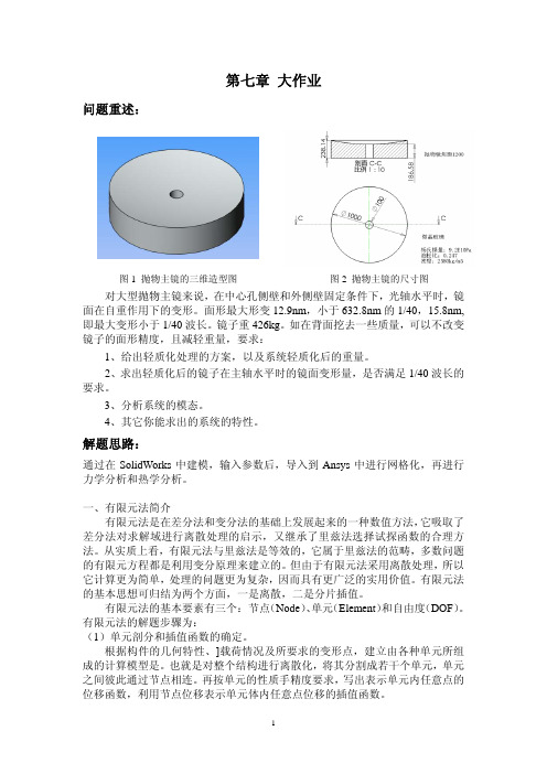
第七章大作业问题重述:图1 抛物主镜的三维造型图图2 抛物主镜的尺寸图对大型抛物主镜来说,在中心孔侧壁和外侧壁固定条件下,光轴水平时,镜面在自重作用下的变形。
面形最大形变12.9nm,小于632.8nm的1/40,15.8nm,即最大变形小于1/40波长。
镜子重426kg。
如在背面挖去一些质量,可以不改变镜子的面形精度,且减轻重量,要求:1、给出轻质化处理的方案,以及系统轻质化后的重量。
2、求出轻质化后的镜子在主轴水平时的镜面变形量,是否满足1/40波长的要求。
3、分析系统的模态。
4、其它你能求出的系统的特性。
解题思路:通过在SolidWorks中建模,输入参数后,导入到Ansys中进行网格化,再进行力学分析和热学分析。
一、有限元法简介有限元法是在差分法和变分法的基础上发展起来的一种数值方法,它吸取了差分法对求解域进行离散处理的启示,又继承了里兹法选择试探函数的合理方法。
从实质上看,有限元法与里兹法是等效的,它属于里兹法的范畴,多数问题的有限元方程都是利用变分原理来建立的。
但由于有限元法采用离散处理,所以它计算更为简单,处理的问题更为复杂,因而具有更广泛的实用价值。
有限元法的基本思想可归结为两个方面,一是离散,二是分片插值。
有限元法的基本要素有三个:节点(Node)、单元(Element)和自由度(DOF)。
有限元法的解题步骤为:(1)单元剖分和插值函数的确定。
根据构件的几何特性、]载荷情况及所要求的变形点,建立由各种单元所组成的计算模型是。
也就是对整个结构进行离散化,将其分割成若干个单元,单元之间彼此通过节点相连。
再按单元的性质手精度要求,写出表示单元内任意点的位移函数,利用节点位移表示单元体内任意点位移的插值函数。
(2)单元特性分析。
把各单元按节点组集成与原结构相似的整体结构,得到整体结构的节点力与节点位移的关系,即整体结构平衡方程组。
(4)求解有限元方程。
引入支承条件,根据不同的计算方法求解有限元方程,得出各节点的位移。
电磁超声表面波产生机理的ANSYS仿真
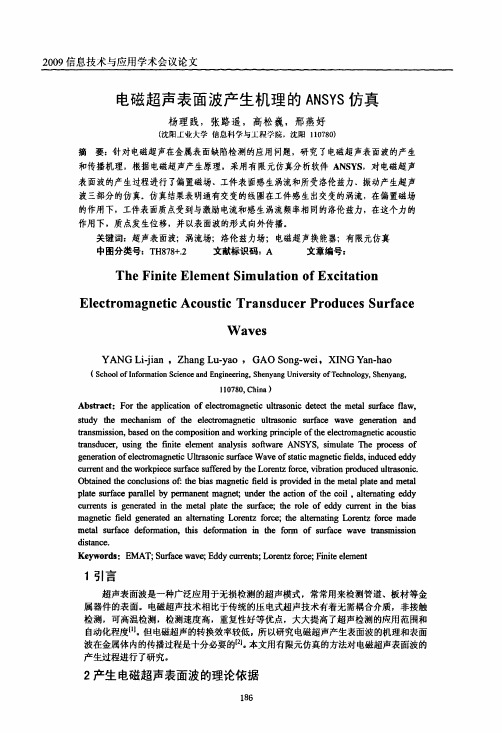
2009信息技术‘j应用学术会议论文田43D—ANSYS建横图4中V1、V2分别为承磁体的N、S极,在水磁体中问有州条通有大小相【司方向相反的变坐电流的导线V4、V5、V6、V7,是下方的大矩彤体V3为被目4钢板。
采用ANSYS仿真软件下的3D磁模型SOLID97单Jc,此单,c定义了8个节点和5个自m度。
定义被测工件为可用于涡流计算的SOLlD971单元,其他无涡流计算的单元选用SOLID970电兀。
线圈中加载屠太值为4安培,频率为800Hz的正弦变变电流,空气层施加约束,进行仿真求解。
在被测工件的趋肤层得到感生涡流,该涡流在永磁体提供的偏置碰场的作用下所产生洛伦兹力。
为了能看到工件巾所形成涡流和受力的大小和^向,在后处理时,绘制涡流和济伦兹力的欠{;}用,如罔5所示。
黼7j:J-。
’。
J“2i。
8。
岔鼍b。
曾73;;。
捌。
j£i。
(-)盒一板中生成的涡漉●●■■■■■二二二==—=———二j2,■一00420㈣4.1260]68LJ210025212*1Ⅲ3781(b)盒一板中的洛怆盐力围5钢板寰面产生的潞渣和洛伦矗力*■圈图5a中所示为被测工件表面感生的涡流.在导线正F方的钢扳表面产生的涡流最太,电流密度达到356066A/m2。
涡流在导线的右侧为顺时针,左侧为逆时针方向。
图5b为被测工件质子所受的洛伦兹山,同样,在导线下方的质点所受的洛伦兹力昂太为0378N。
山于相邻导线通有的电流方向相反,所产生的涡流由向相反,则所受的济伦兹力的方向相反,分别为Y轴的负方向和正方向。
此洛伦蓝力即为超声表面波的被源。
线圈中通过交变的电流激励,因此被测工件表面感生出交变的锅流和洛伦兹力,如酗6所示。
图6为钢板表面一点所通过的电流密度和所受洛伦兹力随时间变化的曲线。
从幽6a可以看出,该点通过的电流密度频率与导线中通过的激励电流的颠率相同,同为800|Iz,而且随着时间的增加,电流密度的幅值逐渐碱小。
而幽6b为改点所受Y方向的力随时何变化的曲线。
ANSYS中的错误

1. Warning:Both solid model and finite element model boundary conditions have been applied to this model. As solid loads are transferred to the nodes or elements, they can overwrite directly applied loads. 解:ANSYS实际上是有两种模型的,一种是几何模型,一种是有限元模型,计算用的是有限元模型,建模时可以建几何模型划分网格得到有限元模型,也可以直接建有限元模型。
而对于载荷的处理,你可以添加到几何模型上,如点、线、面、体,也可以添加到有限元模型上,如节点、单元等,默认的几何模型划分网格时,几何模型上的载荷会转换到有限元模型上,而此时你可能又在有限元模型上添加了载荷,所以会出来提示你检查一下,以免几何模型上的载荷和有限元模型上的载荷冲突以造成overwrite的问题。
如果确定没有问题,这个提示可直接无视。
2. Warning:Shape testing revealed that 481 of the 38538 new or modified elements violate shape warning limits. 解:单元形状奇异,可忽略,但有时计算应力时会出错。
基于有限元方法的多导体传输线电感电容参数的计算
∫∫
B gd S
(7)
通过有限元方法求出所需积分曲面上的磁感应强 度,并利用数值积分的方法求解相应边界条件下 的磁链ψ 1 ,ψ 2 ,L ,ψ n ,带入上式(6)中就可求出 相应的电感值。
Ci 0 =
C ij
qi Ui 0
Ui1 =L Uii−1 =Uii+1L =Uin =0
(3.1)
3 传输线电容电感参数的计算实例
r3 = 0.004m 、 r4 = 0.005m 、 h = 0.126m 。内
绝缘介质的相对介电常数为 ε r = 2.5 ,外绝缘皮 的相对介电常数为 ε r = 2.6 ,所有介质的相对磁 导率为 1。
h = 0.126m ,D = 0.01m ,µr = 1 , 根据式 (6.1)
(6.2)加磁场边界条件,分析导线周围的磁场分 布, 并通过式 (7) 计算所需磁链, 再带入到式 (6.1) (6.2)便得到单位长度电感参数矩阵如式(9)所 示。
(4)
q =
Ò ∫∫
D gd S
通过有限元方法求出所需积分曲面上的电位移矢 量,并利用数值积分的方法求解相应边界条件下 的电荷量 q1 , q2 ,L , qn ,带入上式(3)中就可求 出相应的电容值。 2.2 电感的计算 考虑 n 个载流线圈的回路系统, 空间的磁场是 由 n 个线圈中的电流产生的。在线性磁媒质情况 下,空间的磁感应强度与各线圈中的电流成线性 关系。任一个线圈的磁链与空间磁场成正比,因 此任一个线圈中的磁链与各线圈中电流成线性关 系。且有
[8-10]
等对传输线的参数进行了一系列的
研究。本文基于有限元软件 ANSYS 分析研究了传 输线单位长度的电感、电容,计算结果在精度以 及适用范围上都有一定的优势。
- 1、下载文档前请自行甄别文档内容的完整性,平台不提供额外的编辑、内容补充、找答案等附加服务。
- 2、"仅部分预览"的文档,不可在线预览部分如存在完整性等问题,可反馈申请退款(可完整预览的文档不适用该条件!)。
- 3、如文档侵犯您的权益,请联系客服反馈,我们会尽快为您处理(人工客服工作时间:9:00-18:30)。
Finite Element Simulations with ANSYS Workbench 12 Theory – Applications – Case StudiesHuei-Huang LeeSDCPUBLICATIONSSchroff Development CorporationBetter Textbooks. Lower Prices.Visit the following websites to learn more about this book:46 Chapter 2 Sketching Chapter 2SketchingA simulation project starts with the creation of a geometric model. T o be pro0cient at simulations, an engineer has to be pro0cient at geometric modeling 0rst. In a simulation project, it is not uncommon to take the majority of human-hours to create a geometric model, that is particularly true in a 3D simulation.A complex 3D geometry can be viewed as a collection of simpler 3D solid bodies. Each solid body is often created by 0rst drawi ng a sketch on a plane, and then the sketch i s used to generate the 3D soli d body usi ng tools such as extrude, revolve, sweep, etc. In turn, to be pro0cient at 3D bodies creation, an engineer has to be pro0cient at sketching 0rst.Purpose of the ChapterThe purpose of this chapter is to provide exercises for the students so that they can be pro0cient at sketching using DesignModeler. Five mechanical parts are sketched in this chapters. Although each sketch is used to generate a 3D models, the generation of 3D models is so trivial that we should be able to focus on the 2D sketches without being distracted. More exercises of sketching will be provided in later chapters.About Each SectionEach sketch of a mechani cal part wi ll be completed i n a secti on. Sketches i n the 0rst two secti ons are gui ded i n a step-by-step fashion. Section 1 sketches a cross section of W16x50; the cross section is then extruded to generate a solid model in 3D space. Section 2 sketches a triangular plate; the sketch is then extruded to generate a solid model in 3D space.Secti on 3 does not mean to provi de a hands-on case. It overvi ews the sketchi ng tools i n a systemati c way, attempting to complement what were missed in the 0rst two sections.Sections 4, 5, and 6 provide three cases for more exercises. Sketches in these sections are in a not-so-step-by-step fashion; we purposely leave some room for the students to 0gure out the details.2.1-2 Start Up <DesignModeler>25".628".380"7.07"R.375"[4] Detail dimensions[2] After a while, the <Workbench GUI> shows up.[3] Click the plus sign (+) to expand the <Component Systems>. Note that the plus sign become minussign.[4] Double-click <Geometry> to place a system in the<Project Schematic>.[6] Double-click <Geometry> tostart up DesignModeler.[5] If anything goes wrong, click here to show message.[1] From Start menu, click to launch the Workbench.Notes: In a step-by-step exercise, whenever a circle is used with a speech bubble, it is to indicate that mouse or keynoard ACTIONS must be taken in that step (e.g., [1, 3, 4, 6, 8, 9]). The circle may be small or large, ;lled with white color or un ;lled, depending on whichever gives more information. A speech bubble without a circle (e.g., [2, 7]) or with a rectangle (e.g., [5]) is used for commentary only, no mouse or keyboard actions are needed.2.1-3 Draw a Rectangle on <XYPlane>[9] Click <OK>. Note that, after clicking <OK>, the length unit connot be changed anymore.[8] Select <Inch> as the length unit.[7] After a while, the DesignModeler [1] <XYPlane> is already the current sketchingplane.[2] Click <Sketching> to enter the sketching mode.[4] Click <Rectangle> tool.[3] Click <Look At> to rotate the coordinate axes, so that you face the <XYPlane>.[5] Draw a rectangle (using click-and-drag) roughly like this.Impose symmetry constraints...Specify dimensions...[6] Click<Constraint>toolbox.[8] Click<Symmetry>tool.[9] Click the verticalaxis and then twovertical lines on bothsides to make themsymmetric about thevertical axis.[10] Right-clickanywhere on the graphicarea to open the contextmenu, and choose<Select new symmetryaxis>.[11] Click thehorizontal axis andthen two horizontallines on both sidesto make themsymmetric aboutthe horizontal axis.[7] If you don'tsee <Symmetry>tool, click here toscroll down toreveal the tool.[12] Click<Dimensions>toolbox.[13] Leave<General> as the default tool.[17] In the<Detai ls Vi ew>, type 7.07 (in) for H1 and 16.25 (in)for V2.[14] Click this line,move the mouseupward, and click againto create H1.[15] Click this line,move the mouserightward, and clickagain to create V2.[17] Click<Zoom to Fit>.[16] The segments turn toblue color. Colors are usedto indicate the constraintstatus. The blue color meansthat the geometric entitiesare well constrained.The ruler occupies space and is sometimes annoying; let's turn it off...Let's display dimension values (in stead of names) on the graphic area...[2] The ruler disappears. It creates more space for the graphic area. For the rest of the book, we always turn off the ruler to make more space in the graphic area.[1] Pull-down-select <View/Ruler> to turn the ruler off.[3] If you don't see <Display> tool, click here to scroll all the way down to the bottom.[4] Click <Display> tool.[5] Click <Name> to turn it off. The <Value> automatically turns on.[6] The di mensi on names are replaced by the values. For the rest of the book, we always display values instead of names, so that the sketching will be more ef8cient.Draw a polyline; the dimensions are not important for now...Copy the newly created polyline to the right side, ;ip horizontally...2.1-6 Copy the Polyline[1] Select <Draw> toolbox.[2] Select <Polyline> tool.[3] Click roughly here to start the polyline. Make sure a <C> (coincident) appearsbefore clicking.[4] Click the second point roughly here. Make sure an <H> (horizontal) appearsbefore clicking.[5] Click the third point roughly here. Make sure a <V> (vertical) appears before clicking.[6] Click the last point roughly here. Make sure an <H> and a <C> appearbefore clicking.[7] Right-click anywhere on the graphic area to open the context menu, and select <Open End> to end the <Polyline> tool.[4] Right-click anywhere on the graphic area to open the context menu, and select <End/Use Plane Origin asHandle>.[1] Select <Modify> toolbox.[2] Select <Copy> tool.[3] Control-click (see [11, 12]) the three newly created segments one by one.Context menu is used heavily...Basic Mouse OperationsAt this point, let's look into some basic mouse operations [10-16]. Skill of these operations is one of the keys to be pro<cient at geometric modeling.[8] Right-click anywhere to open the context menu again and select <End> to end the <Copy> tool. An alternative way (and better way) is to press ESC to end a tool.[9] The horizontally =ipped polyline has been copied.[6] Right-click anywhere to open the context menu again and select <Flip Horizontal>.[5] The tool automatically changes from <Copy> to<Paste>.[7] Right-click anywhere to open the context menu again and select <Paste at PlaneOrigin>.[10] Click: singleselection[11] Control-click: add/remove selection [12] Click-sweep: continuous selection.[13] Right-click: open context menu.[14] Right-click-drag:box zoom.[15] Scroll-wheel: zoom in/out.[16] Middle-click-drag:rotation.rim Away Unwanted Segments2.1-8 Impose Symmetry Constraints[3] Click this segment to trim it away.[4] And click this segment to trim it away.[1] Select <T rim>tool.urn on <Ignore Axis>. If you don't turn it on, the axes will be treated as trimming tools.[2] Select <Symmetry>.[3] Click thishorizontal axis and then two horizontal segments on both sides as shownto make them symmetric about the horizontal axis.[1] Select <Constraints> toolbox.[4] Right-click anywhere to open the context menu and select <Select new symmetryaxis>[5] Click this vertical axis and then two vertical segments on both sides as shown to make them symmetric about the vertical axis. They seemed already symmetric before we impose this constraint, but the symmetry is "weak" and may be overridden (destroyed)by other constraints.[2] Leave <General> as default tool.<Dimensions> toolbox.[4] Select <Horizontal>.[3] Click this segment and move leftward to create a vertical dimension. Note that the entity isblue-colored.[5] Click these two segments sequentially and move upward tocreate a horizontal dimension.[6] T ype 0.38 for H4 and 0.628 for V3.2.1-11 Move Dimensionstoolbox.[2] Select <Fillet> tool.[3] T ype 0.375 for the :llet radius.[4] Click two adjacent segments sequentially to create a :llet. Repeat this step for other three corners.[2] Select <Move>.[3] Click a dimension value and move to a suitable position as you like. Repeat this step for other dimensions.[1] Select <Dimensions> toolbox.[5] The greenish-blue color of the :llets indicates that these :llets are under-constrained. The radius speci:ed in [3] is a "weak" dimension (may be destroyed by other constraints). Y ou could impose a <Radius> (which is in <Dimension> toolbox) to turn the :llets to blue. We, however, decide to ignore the color. We want toshow that an under-constrained sketch can stillbe used. In general, however, it is a good practice to well-constrain all entitiesin a sketch.[9] Click <Zoom to Fit> whenever needed.[10] Click <Display Plane> to switch off the display of sketching plane.[11] Click all plus signs (+) to expand the model tree and examine the <T ree Outline>.[6] Active sketch is shown here.[5] The active sketch(Sketch1) is automatically chosen as <Base Object> you can change to other sketch if needed.[2] The model is now in isometricview.[4] Note that the <Modeling> mode is automatically activated.[7] T ype 120 (in) for <Depth>[1] Click the little cyan sphere to rotate the model in isometric view for a better visual effect.[3] Click <Extrude>.[8] Click <Generate>[1] Click <SaveProject>. T ype"W16x50" as projectname.[2] Pull-down-select<File/CloseDesignModeler> toclose DesignModeler.[3] Alternatively youcan click <SaveProject> in the<Workbench GUI>.[4] Pull-down-select<File/Exit> toexi t Workbench.riangular Platemm30 mm300 mm2.2-2 Start up <DesignModeler>[1] From Start menu, launch the <Workbench>[2] Double-click tocreate a <Geometry>system.[3] Double-click tostart up<DesignModeler>.[1] Thehas threeplanes ofsymmetry.[2] Radii ofthe 7lletsare 10 mm.[3] Forces areapplied oneach side face.2.2-3 Draw a T riangle on <XYPlane>[6] Select <Sketching> mode.[7] Click <Look At> to look at <XYPlane>.[5] Pull-down-select <View/Ruler> to turn the ruler off. For the rest of the book, we always turn off the ruler to make more space in the graphicarea.[4] Select <Millimeter> as length unit.[2] Click roughly here to start a polyline.[3] Click the second point roughly here. Make sure a <V> (vertical) constraint appears beforeclicking.[4] Click the third point roughly here. Make sure a <C> (coincident) constraint appears before clicking. <Auto Constraints> is an important feature of DesignModeler and will be discussed in Section 2.3-5.[5] Right-click anywhere to open the context menu and select <Close End> to close the polyline andend the tool.[1] Select <Polyline> from <Draw> toolbox.Before we proceed, let's spend a few minutes looking into some useful tools for 2D graphics controls [1-10]; feel free to use these tools whenever needed. The tools are numbered according to roughly their frequency of use. Note that more useful mouse short-cuts for <Pan>, <Zoom>, and <Box Zoom> are available; please see Section 2.3-4.2.2-4 Make the T riangle Regular2.2-5 2D Graphics Controls[1] Select <Equal Length> from <Constraints> toolbox.[2] Click these two segments one after the other to make their lengths equal.[3] Click these two segments one after the other to make their lengths equal.[9] <Undo>. Click this tool to undo what you've just done. Multiple undo is possible. This tool is [10] <Redo>. Click this tool to redo what you've just undone. This tool is [2] <Zoom to Fit>. Click this tool to Bt the entire sketch in the graphic area.[4] <Box Zoom>. Click to turn on/off this mode. Y ou can click-and-drag a box on the graphic area to enlarge that portion of graphics.[5] <Zoom>. Click to turn on/off this mode. Y ou can click-and-drag upward or downward on the graphic area to zoom in or out.[1] <Look At>. Click this tool to make current sketching plane rotate towardyou.[6] <Previous View>. Click this tool to go to the previous view.[7] <Next View>. Click this tool to go to the next view.[8] These tools work in both <Sketching> or <Modeling> mode.[3] <Pan>. Click to turn on/off this mode. Y ou can click-and-drag on the graphic area tomove the sketch.2.2-7 Draw an Arc[2] Select <Horizontal>.[6] Select <Move> and thenmove the dimensions as you like (Section2.1-11).[1] Click <Display> in the<Dimension> toolbox. Click <Name> to switch it off and turn <Value> on. For the rest of the book, we always display values instead of names.[3] Click the vertex on the left and the vertical line on the right sequentially, and then move the mouse downward to create this dimension. Before clicking, make sure the cursor changes to indicate that the point or edge has been"snapped."[4] Click the vertex on the left and the vertical axis, and then move the mouse downward to create this dimension. Note thatthe triangle turns to blue, indicating they are well de =nednow.[5] In the <Details View>, type 300 and 200 for the dimensions just created. Click <Zoom to Fit>(2.2-5[2]).[2] Click this vertex as the arc center. Make sure a <P> (point) constraint appears before clicking.[3] Click the second point roughly here. Make sure a <C> (coincident) constraint appears before clicking.[4] Click the third point here. Make sure a <C> (coincident) constraint appears before clicking.[1] Select <Arc by Center> from <Draw> toolbox.2.2-6 Specify Dimensions[2] Click thearc.[1] Select <Replicate> from <Modify> toolbox. T ype 120 (degrees) for <r>. <Replicate> is equivalent to <Copy>+<Paste>.[7] Whenever you have dif<culty making <P> appear, click <Selection Filter: Points> in the toolbar. The <Selection Filter> also can be set from the context menu,see [8].Handle> in the context menu.[8] The <Selecti on Filter> also can be set from the contextmenu.[5] Right-click-select<Rotate by r Degrees> from the context menu.[6] Click this vertex to paste the arc. Make sure a <P> appears before clicking. If you have dif<culty making <P> appear, see [7, 8].For instructional purpose, we chose to manually set the paste handle [3] on the vertex [4]. We could have used plane origin as handle. In fact, that would have been easier since we wouldn't have to struggle to make sure whether a <P> appears or not. Whenever you have dif ;culty to "snap" a parti cular poi nt, you should take advantage of <Selecti on Filter> [7, 8].2.2-9 T rim Away Unwanted Segments[10] Click this vertex to paste the arc. Make sure a <P> appears before clicking (see [7, 8]).[9] Right-click-select<Rotate by r Degrees> in the context menu.[11] Right-click-select <End> in the context menu to end <Replicate> tool. Alternatively, you may press ESC to end atool.[3] Click to trim unwanted segments as shown, totally 6 segments are trimmed away.[1] Select <T rim> from <Modify> toolbox.[2] T urn on <Ignore Axis>.2.2-11 Specify Dimension of Side FacesAfter impose dimension in [2], the arcs turns to blue, indicating they are well de ;ned now. Note that we didn't specify the radii of the arcs; after wellde ;ned, the radii of the arcs can be calculated from other dimensions.Constraint StatusNote the arcs have a greenish-blue color, indicating they are not well de ;ned yet (i.e., under-constrained). Other color codes are: blue and blackcolors for well de ;ned entities (i.e., ;xed in the space); red color for over-constrained entities; gray to indicate an inconsistency.[1] Select <Equal Length> from <Constraints> toolbox[5] Click the horizontal axis as the line of symmetry.[4] Select <Symmetry>.[2] Click this segment and the vertical segment sequentially to make theirlengths equal.[3] Click this segment and the vertical segment sequentially to make theirlengths equal.[6] Click the lower and upper arcs sequentially tomake them symmetric.[1] Select <Dimension> toolbox and leave <General> as default.[2] Click the vertical segment and move the mouse rightward tocreate this dimension.[3] T ype 40 for the dimension just created.2.2-10 Impose Constraints[1] Select <Offset> from <Modify> toolbox.[2] Sweep-select all the segments (sweep each segment while holding your left mouse button down, see 2.1-6[12]). After selected, the segments turn to yellow. Sweep-select is alsocalled paint-select.[4] Right-click-select <End selection/Place Offset> in the context menu.[6] Right-click-select <End> in the context menu, or press ESC, to close <Offset>tool.[5] Click roughly here to place theoffset.[3] Another way to select multiple entities is to switch the<Select Mode> to <Box Select>, and then draw a box to select all entities inside the box.2.2-13 Create Fillets[1] Select <Fillet> in <Modify> toolbox. T ype 10 (mm) for the<Radius>.[7] Select <Horizontal> from <Dimension> toolbox.[8] Click the two left arcs and move downward to create this dimension. Note the offsetturns to blue.[9] T ype 30 for the dimension just created.[10] It is possible that these two point become separate now. If so, impose a <Coincident> constraint on them, see [11].[11] If necessary,impose a <Coincident> on the separate points.[2] Click These two segments sequentially to create a 7llet. Repeat this step to create the other two 7llets. Note that the 7llets are in greenish-blue color, indicating they are notwell de7ned yet.2.2-14 Extrude to Create 3D Solid[4] Select <Radius> from <Dimension> toolbox.[3] Dimensions speci6ed in a toolbox are usually regarded as "weak"dimensions, meaning they may be changed by imposing other constraints or dimensions.[5] Click one of the 6llets and move upward to create this dimension. This action turns a "weak" dimension to a "strong" one. The 6lletsturn blue now.[2] Click <Extrude>.[1] Click the little cyan sphere to rotate the model in isometric view, to have a better view.[3] T ype 10 (mm) for <Depth>.[4] Click <Generate>.[5] Click <Display Plane> to turn off the display ofsketching plane.[6] Click all plus signs (+) to expand and examine the <T ree Outline>.[1] Click <SaveProject>. T ype"T riplate" as projectname.[2] Pull-down-select<File/CloseDesignModeler> toclose DesignModeler.[3] Alternatively youcan click <SaveProject> in the<Workbench GUI>.[4] Pull-down-select<File/Exit> toexi t Workbench.reeree Outline> contains an outline of the model tree , the tree representation of the geometric model. Each leaf of the tree is called an object . A branch is an object containing one or more objects under itself. A model tree consists of planes , features , and a part branch. The parts are the only objects that are exported to <Mechanical>. ng an object and select a tool from the context menu, you can operate on the object, such as delete, rename, duplicate, etc.[1] Pull-down menusand toolbars.ree Outline>, in <Modeling> mode.[6] <Details View>.[5] Graphics area.[7] Status bar[4] <Sketching T oolboxes> in <Sketching> mode.[2] Mode tabs.[8] A separator allow you to resize the window panes.A sketch consists of points and edges ; edges may be straight lines or curves. Along with these geometric entities, there are dimensions and constraints imposed on these entities. As mentioned (Section 2.3-2), multiple sketches may be created on a plane. T o create a new sketch on a plane on whi ch there i s yet no sketches, you si mply swi <Sketching> mode and draw any geometric entities on it. Later, if you want to add a new sketch on that plane, you need to click <New Sketch> [3]. Only one plane and one sketch is active at a time [1, 2]: newly created sketches are added to the active plane, and newly created geometric entities are added to the active sketch. In this chapter, we only work wi th a si ngle sketch whi ch i s on the <XYPlane>. More on creati ng sketches wi ll be di scussed i n Chapter 4. 2.3-3 Sketchesactive plane is <XYPlane> <New Plane> to create a new plane.[3] Y ou can choose many ways of creating a newplane.Sketch> to create a sketch on the active sketching plane.active sketchingplane.active sketch.[4] Active sketching plane can be changed using the pull-down list, or by selection from the<T ree Outline>.[5] Active sketch can be changed using the pull-down list, or by selectionfrom the <T ree Outline>.toolbox.[3] <Dimensions>toolbox.toolbox.[5] <Settings>toolbox.[1] By default,DesignModeler is in<Auto Constraints> mode, both globally andlocally. Y ou can turnthem off whenevercause troubles. [1] <Draw>toolbox.[2] Right-click andselect one of theoptions to complete the<Spline> tool.[1] <Modify>toolbox.[2] Contextmenu for<Split> tool.[3] Contextmenu for <SplineEdit>.toolbox. [1] <Constraints>toolbox.the grid display.References1. ANSYS Help System>DesignModeler>2D Sketching>Auto Constraints2. ANSYS Help System>DesignModeler>2D Sketching>Constraints3. ANSYS Help System>DesignModeler>2D Sketching>Draw4. ANSYS Help System>DesignModeler>2D Sketching>Modify5. ANSYS Help System>DesignModeler>2D Sketching>Dimensions6. ANSYS Help System>DesignModeler>2D Sketching>Constraints7. ANSYS Help System>DesignModeler>2D Sketching>Settings toolbox.[3]the snap capability.[4] If you turn onthe grid display, youcan specify the gridle the nut has i nternal threads. Thi sd body for a porti on of the bolt [1] In Section 3.2, we will use this sketch again to generate a 2D solid model. The 2DExternal threads (bolt)Internalthreads(nut)H 8pMinor diameter of internal thread d1Nominal diameter d 60o[1] The threaded boltcreated in thisexercise.[1] Draw ahorizontal linewith dimensionsas shown.ons (30o, 60o, 60o, 0.541, and 2.165) as shown below. Note that, to avoid confusion, we explicitly specify all the dimensions. Y ou may apply constraints instead. For example, using <Parallel> constraint in stead of specifying an angle dimension [1].[1] Y ou may impose a<Parallel> constrainton this line instead ofspecifying the angle.rim Unwanted Segments2.4-6 Replicate 10 TimesSelect all segments except the horizontal one (totally 4 segments), and replicate 10 times. Y ou may need to manually<Selection Filter: Points> [2].[1] T angentpoint. [1] Set Paste Handle at thispoint.[1] The sketch after trimming.The Finite Element Method in Machine Design , Prentice-Hall, 1992; Chapter 7. Threaded Fasteners.Machine Design: Theory and Practice , Macmillan Publishing Co.,[1] Create this segment by using <Replicate>.[2] Draw this segment, which passes through the origin.[4] Draw this vertical segment. Y ou can trim it after next step.[5] Draw this horizontal segment.The 8gure below shows a pair of identical spur gears in mesh [1-12]. Spur gears have their teeth cut parallel to the axis of the shaft on which the gears are mounted. Spur gears are used to transmit power between parallel shafts. In o, they must sati sfy the fundamental law of point of contact between two teeth This 8xed point is called the pitch point [6].for a mechanical engineer. However, if you are not concerned about these geometric details for now, you may skip the 8rst two subsections and jump directly to Subsection 2.5-3.[7] Common tangent of the pitch circles.[6] Contact point (pitch point).[3] Pitch circle [9] Addendum vi ng gear rotates clockwise.[4] Pitch circle of the driving gear.[5] Line of centers.[12] The has a radius of[11] The shaft has a radius of 1.25 in.dimensions as shown (the vertical dimensions are measured down to the X-axis). Note that the dimension values display three digits after decimal point, but we actually typed with @ve digits (refer to the above table). Impose a <Coincident> constraint on the Y-axis for the-coordinate of 2.500.Connect these six points using <Spline> tool, keeping <Flexible> option on, and close the spline with <Open End>. Note that you could draw <Spline> directly without creating <Construction Points> @rst, but2.5-4 Draw CirclesDraw three circles [1-3]. Let the outermost construction point [3]. Specify radii for the circle of shaft (1.25 in) and the dedendum circle 2.5-5 Complete the Pro4leDraw a line starting from the lowestconstruction point, and make it perpendicular to the dedendum circle [1-2]. Note that, when drawing the line, avoid a <V> auto-constraint. Draw a 4llet [3] of radius 0.1 in to [3] Let addendum circle "snap" to the outermost construction point.[1] The circle ofshaft.[2] Dedendumcircle.This segment is a straight line and perpendicular to the dedendum circle.[3] This 4llet has a radius of 0.1 in.[1] Dedendum circle.[1] Replicatedpro:le.Times Project>Section 2.5 Exercise: Spur Gears 85References1. Deutschman, A. D., Michels, W . J., and Wilson, C. E., Machine Design: Theory and Practice , Macmillan Publishing Co.,Inc., 1975; Chapter 10. Spur Gears.2. Zahavi, E., The Finite Element Method in Machine Design , Prentice-Hall, 1992; Chapter 9. Spur Gears.2.5-8 Trim Away Unwanted Segments2.5-9 Extrude to Create 3D SolidExtrude the sketch 1.0 inch to create a 3D solid as shown. Save the project and exit from <Workbench>. We will resume this project again in Section 3.4.T rim away unwanted portion on the addendum circle and the dedendum circle.。