5外文翻译原文
桥梁毕业设计外文翻译5
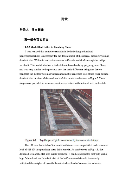
附录附录A 外文翻译第一部分英文原文4.2.2 Model that Failed in Punching ShearIt was realized that complete restraint in both the longitudinal and transversedirections is necessary for the development of the internal arching system in the deck slab. With this realization,another half-scale model of a two-girder bridge was built. This model also had a deck slab reinforced only by polypropylene fibres, and was very similar to the previous one, the main difference being that the top flangesof the girders were now interconnected by transverse steel straps lying outside the deck slab. A view of the steel work of this model can be seen in Fig. 4.7.These straps were provided so as to serve as transverse ties to the internal arch in the slab.The 100 mm thick slab of the model with transverse straps failed under a central load of 418 kN in a punching-shear failure mode. As can be seen in Fig. 4.8, the damaged area of the slab was highly localized. It can be appreciated that with such a high failure load, the thin deck slab of the half-scale model could have easily withstood the weights of even the heaviest wheel load of commercial vehicles.The model tests described above and in sub-section 4.2.1 clearly demonstrate that an internal arching action will indeed develop in a deck slab, but only if it is suitably restrained.4.2.3 Edge StiffeningA further appreciation of the deck slab arching action is provided by tests on a scale model of a skew slab-on-girder bridge. As will be discussed in sub-section 4.4.2, one transverse free edge of the deck slab of this model was stiffened by a composite steel channel with its web in the vertical plane. The other free edge was stiffened by a steel channel diaphragm with its web horizontal and connected to the deck slab through shear connectors. The deck slab near the former transverse edge failed in a mode that was a hybrid between punching shear and flexure. Tests near the composite diaphragm led to failure at a much higher load in punching shear (Bakht and Agarwal, 1993).The above tests confirmed yet again that the presence of the internal arching action in deck slabs induces high in-plane force effects which in turn demand stiffer restraint in the plane of the deck than in the out-of-plane direction.4.3 INTERNALLY RESTRAINED DECK SLABSDeck slabs which require embedded reinforcement for strength will now be referred to as internally restrained deck slabs. The state-of-art up to 1986 relating to the quantification and utilization of the beneficial internal arching action in deck slabs with steel reinforcement has been provided by Bakht and Markovic (1986). Their conclusions complemented with up-to-date information are presented in this chapter in a generally chronological order which, however, cannot be adhered to rigidlybecause of the simultaneous occurrence of some developments.4.3.1 Static Tests on Scale ModelsAbout three decades ago, the Structures Research Office of the Ministry of Transportation of Ontario (MTO), Canada, sponsored an extensive laboratory-based research program into the load carrying capacity of deck slabs; this research program was carried out at Queen's University, Kingston, Ontario. Most of this research was conducted through static tests on scale models of slab-on-girder bridges. This pioneering work is reported by Hewitt and Batchelor (1975) and later by Batchelor et al. (1985), and is summarized in the following.The inability of the concrete to sustain tensile strains, which leads to cracking, has been shown to be the main attribute which causes the compressive membrane forces to develop. This phenomenon is illustrated in Fig. 4.9 (a) which shows the part cross-section of slab-on-girder bridge under the action of a concentrated load.The cracking of the concrete, as shown in the figure, results in a net compressive force near the bottom face of the slab at each of the two girder locations. Midway between the girders, the net compressive force moves towards the top of the slab. It can be readily visualized that the transition of the net compressive force from near the top in the middle region, to near the bottom at the supports corresponds to the familiar arching action. Because of this internal arching action, the failure mode of a deck slab under a concentrated load becomes that of punching shear.If the material of the deck slab has the same stress-strain characteristics in both tension and compression, the slab will not crack and, as shown in Fig. 4.9 (b), will not develop the net compressive force and hence the arching action.In the punching shear type of failure, a frustum separates from the rest of the slab, as shown in schematically in Fig. 4.10. It is noted that in most failure tests, the diameter of the lower end of the frustrum extends to the vicinity of the girders.From analytical and confirmatory laboratory studies, it was established that the most significant factor influencing the failure load of a concrete deck slab is the confinement of the panel under consideration. It was concluded that this confinement is provided by the expanse of the slab beyond the loaded area; its degree was founddifficult to assess analytically. A restraint factor, η, was used as an empirical measure of the confinement; its value is equal to zero for the case of no confinement and 1.0 for full confinement.The effect of various parameters on the failure load can be seen in Table 4.1, which lists the theoretical failure loads for various cases. It can be seen that an increase of the restraint factor from 0.0 to 0.5 results in a very large increase in the failure load. The table also emphasizes the fact that neglect of the restraint factor causes a gross underestimation of the failure load.It was concluded that design for flexure leads to the inclusion of large amounts of unnecessary steel reinforcement in the deck slabs, and that even the minimum amount of steel required for crack control against volumetric changes in concrete is adequate to sustain modern-day, and even future, highway vehicles of North America.It was recommended that for new construction, the reinforcement in a deck slab should be in two layers, with each layer consisting of an orthogonal mesh having the same area of reinforcement in each direction. The area of steel reinforcement in each direction of a mesh was suggested to be 0.2% of the effective area of cross-section of the slab. This empirical method of design was recommended for deck slabs with certain constraints.4.3.2 Pulsating Load Tests on Scale ModelsTo study the fatigue strength of deck slabs with reduced reinforcement, five small scale models with different reinforcement ratios in different panels were tested at the Queen's University at Kingston. Details of this study are reported by Batchelor et al. (1978).Experimental investigation confirmed that for loads normally encountered in North America deck slabs with both conventional and recommended reducedreinforcement have large reserve strengths against failure by fatigue. It was confirmed that the reinforcement in the deck slab should be as noted in sub-section 4.3.1. It is recalled that the 0.2% reinforcement requires that the deck slab must have a minimum restraint factor of 0.5.The work of Okada, et al. (1978) also deals with fatigue tests on full scale models of deck slabs and segments of severely cracked slab removed from eight to ten year old bridges. The application of these test results to deck slabs of actual bridges is open to question because test specimens were removed from the original structures in such a way that they did not retain the confinement necessary for the development of the arching action.4.3.3 Field TestingAlong with the studies described in the preceding sub-section, a program of field testing of the deck slabs of in-service bridges was undertaken by the Structures Research Office of the MTO. The testing consisted of subjecting deck slabs to single concentrated loads, simulating wheel loads, and monitoring the load-deflection characteristics of the slab. The testing is reported by Csagoly et al. (1978) and details of the testing equipment are given by Bakht and Csagoly (1979).Values of the restraint factor, η, were back-calculated from measured deflections.A summary of test results, given in Table 4.2, shows that the average value of η in composite bridges is greater than 0.75, while that for non-composite bridges is 0.42. It was concluded that for new construction, the restraint factor, η, can be assumed to have a minimum value of 0.5.Bakht (1981) reports that after the first application of a test load of high magnitude on deck slabs of existing bridges, a small residual deflection was observed in most cases. Subsequent applications of the same load did not result in further residual deflections. It is postulated that the residual deflections are caused by cracking of the concrete which, as discussed earlier, accompanies the development of the internal arching action. The residual deflections after the first cycle of loading suggest that either the slab was never subjected to loads high enough to cause cracking, or the cracks have 'healed' with time.第二部分汉语翻译4.2.2 在冲切剪应力下的实效模型我们已经知道在桥面板内部拱形系统的形成中,不仅纵向而且横向也被完全约束限制是完全必要的。
中国的对外贸易外文翻译及原文
外文翻译原文Foreign T rade o f ChinaMaterial Source:W anfang Database Author:Hitomi Iizaka1.IntroductionOn December11,2001,China officially joined the World T rade Organization(WTO)and be c a me its143rd member.China’s presence in the worl d economy will continue to grow and deepen.The foreign trade sector plays an important andmultifaceted role in China’s economic development.At the same time, China’s expanded role in the world economy is beneficial t o all its trading partners. Regions that trade with China benefit from cheaper and mor e varieties of imported consumer goods,raw materials and intermediate products.China is also a large and growing export market.While the entry of any major trading nation in the global trading system can create a process of adjustment,the o u t c o me is fundamentally a win-win situation.In this p aper we would like t o provide a survey of the various institutions,laws and characteristics of China’s trade.Among some of the findings, we can highlight thefollowing:•In2001,total trade to gross domestic pr oduct(GDP)ratio in China is44%•In2001,47%of Chinese trade is processed trade1•In2001,51%of Chinese trade is conduct ed by foreign firms in China2•In2001,36%of Chinese exports originate from Gu an gdon g province•In2001,39%of China’s exports go through Hong Kong to be re-exported elsewhere2.Evolution of China’s Trade RegimeEqually remarkable are the changes in the commodity composition of China’s exports and imports.Table2a shows China’s annu al export volumes of primary goods and manufactured goods over time.In1980,primary goods accounted for 50.3%of China’s exports and manufactured goods accounted for49.7%.Although the share of primary good declines slightly during the first half of1980’s,it remains at50.6%in1985.Since then,exports of manufactured goods have grown at a muchfaster rate than exports of primary goods.As a result,the share of manufactur ed goods increased t o90.1%,and that of primary good decr eased to9.9%by2001.Also shown in those tables are five subgr oups for manufactur ed goods and primary goods.China’s export was highly dependent on its exports of coal, petroleum,and petr oleum products until mid-80s.The large export volume of petr oleum was also support ed by a sharp rise in oil prices during the period.In1985, the share of mineral fuels is26.1%.In1986,the su d d en decline in the share of primary goods in total exports occurs,which is largely associated with the decline in the export volume of mineral fuels.The price reforms coupled with the declined world petr oleum price areattributable t o the decline.Domestic agriculture production expanded during the1980’s in response to the higher prices thr ough the price reforms and mo r e opportunities given t o the producers to market their products.Although the share of food and live animals in total exports has declined over time,China has become a net exporter of such products since1984.T urning to the manufactur ed goods,the large increase in the share of the manufactur ed goods in the total exports since mid-80s is largely accounted for by the increase in the export in the textile category and the miscellaneous products category.These two gr oups include labor-intensive products such as textiles,apparel, footwear,and toys and sporting goods.During the1990s,the category that exhibited the mos t significant surge in exports is machinery and transport equipment.Its share exp anded from9.0%in1990t o35.7%in2001.3.China’s Processing Trade and Trade by For eign Invested FirmsChina established the legal framework for processing and assembly arrangements in1979.Since then,China has built up considerable strengths in assembling and processing of industrial parts and components.It covers a wide range of industries such as electric machinery,automobile,aerospace,and shipbuilding.T able3a and T able3b demonstrate the amount of processing exports and imports and the importance of stateowned enterprises(SOEs)and foreign-invested enterprises(FIEs)in such forms of trade for1995-2001. Throughout the period from1995to2001,the shares of these two types of processing exports exceed more than half of China’s total exports.In2001,processing exports account for55.4%of the total exports.As is seen in T able3a, process&assembling was dominat ed by SOEs in1995.However,the tr end has been changing.The share of SOEs in process&assembling has been steadilydeclining over the years from84%in1995to62%in2001.The other type of trade, process with imported materials was largely conducted by FIEs and their shares have been gradually increasing from81%in1995to88%in2001.In China’s imports(see T able3b),processing trade is relatively small comp a r ed to exports. After it peak ed at49%in1997,processed imports decline to39%in2001.The decreasing importance of SOEs can be seen in China’s imports as well.Shares by SOEs decr eased from81%in1995t o58%in2001for process&assembling,and from18%to7%for process with imported materials.The decr eased role for SOEs in processing trade may reflect the inefficiency in conducting their business.Since 1997,the Chinese government decided t o implement the shareholding system and t o sell a large numbe r of medium-and small-sized SOEs to the private sector.A n u mbe r of larger enterprise gr oups will be established in various industries thr ough mergers,acquisitions,and leasing and contracting.The restructuring of SOEs is intended to increase profits and to improve their competitive edge.4.China’s Tr ade by Provinces and RegionsA regional breakdown of exports and imports reveals important characteristics of the foreign trade in China.In1997,89.1%of the total exports came from the Eastern region of China(Beijing,Tianjin,Heibei,Lioaning,Guangxi,Shanghai, Jiangsu,Zhejiang,Fujian,Shangdong,Guandong and Hainan).Within the East,the Southeast region accounts for76.3%of China's exports in1997.4Gu ang dong alone pr oduces41.6%of the total exports for the sa me year.Such regional imbalances in exporting activities persist to the present day.In2001,Guandong's share of the national exports is36.0%.For the Southeast and the East,the shares are respectively 79.0%and91.1%.This imbalance of the regional growth in foreign trade may partially be attributed t o the various geographic-specific and sequential o pen-d oo r policies China has exercised thr oughout the last twenty years.The strong growth of th e export sector in the coastal area has been support ed by the massive use of foreign direct investment(FDI).FDI was first attracted by the creation of the Special Economic Zones(SEZ).FDI was concentrated in the provinces of the Southeast coast,namely,Guandong and Fujian.The multinational enterprises that are export-oriented or use adv anced technologies are able to enjoy various preferential policies in the SEZs,such as r educed or ex empt e d corporate income tax,exemption from import tariffs on imported equipment and raw materials.In1984,fourteen coastal cities were opened and were grant ed similar policies as SEZs.Out of thosefourteen cities,ten are located in the Southeast coast regions and four are in the rest of the Eastern regions.Furthermore in1985,similar preferential policies were grant ed t o other coastal economic regions,Pearl River Delta,Y angtze River Delta and Minnan Delta which is t o the south of Fujian.In1990,Pu d o n g in Shanghai was opened and was grant ed extensive preferential policies.Since1984,the Chinese government established thirty-two national-level Economic and T echnological Development Zones(ETDZs).The share of exports in The Y angtze River Delta,the home of Shanghai and two provinces,Jiangsu and Zhejiang has grown steadily during the period1997to 2001.The share of those three regions grew to10.1%,11.0%,and9.1%in2001 from8.1%,7.9%and5.9%in1997,respectively.As the role of high-tech industry beco mes mo r e significant in China’s output and China’s comparative advantage in skilled-labor and capital-intensive industries beco mes higher,the Y angtze River Delta be co mes a new magnet for investment by foreign enterprises.These foreign investments in turn lead to mo r e export and trade.5.Foreign T rade by Major World RegionsUsing China’s official statistics,Table4a and4b highlight merchandise export s and imports t o and from major world regions for1993-2001:Asia,Africa,Europe, Latin America,North America and Oceania.As we see from Table4a,China’s most important export region has always been Asia,which absorbs53%of China’s exports in2001.However,their share of absorption declines from almost62%,their peak level of1995.The importance of North America and Europe in China’s exports, however,has been increasing since1998.In2001,North America takes in mo r e than22%of exports and Europe takes in mo r e than18%.6.China’s Merchandise Exports and Imports by Major Trading PartnersTable5a and Table5b document China’s merchandise exports to and imports from its major trading partners,using China’s official statistics.According to Tabl e 5a,the major exports markets for China in2001are:the United States(20.4%), Hong Kong(17.5%),Japan(16.9%)and the European Union(15.4%).It is well-known that a large proportion of Chinese exports to Hong Kong are re-exported elsewhere so that the true size of the Hong Kong export market has t o be estimated. T o save space for this paper,we will just rely on the official Chinese figures.6Even without adjusting for re-exports,the United States in2001is the largest export market for China.Thus,from an international trade perspective alone,the most important bilateral trade relationship for China is the relationship with the UnitedStates.T ogether t he United States,Hong Kong,Japan and the European Union take in70.2%of China’s exports in2001.Within ASEAN(Association of Southeast Asian Nations),Singapore has been the largest export market for China.In2001, 31.5%of China’s total exports to ASEAN is destined for Singapore.Within the European Union(EU),Germany is the largest market with23.8%of the total Chinese exports going to the EU.9.ConclusionIn the future,we see that there are at least two challenges facing China in the area of international trade.First,with China’s competitiveness growing,many countries will perceive that their producers will no t be able to c o mpe t e with the Chinese exports,either in the third market or in their own domestic market.The backlash will take the form of an increased use of anti-dumping duties and safeguards.W e have already seen the use of such trade instruments against China from a variety of countries,including Japan,the European Union and the United States.A relatively new development is that even developing countries such as India and Mexico are using anti-dumping measur es against Chinese exports to their countries.The difficulty with anti-dumping duties is that they are generally WT O-consistent.Thus joining the WTO d o es no t mean that other countries will reduce their use of anti-dumping duties against China.A second challenge facing China is how t o manage its trade relationship with the United States.The United States is the largest economy on earth.The United States is China’s largest export market.It is also a critical source of technology.A stable and healthy relationship with the United States is important for China’s economic development.It is always a difficult adjustment process for countries to accept a newly e mer gen t economic power.The United States as well as other countries may perceive China as a potential economic threat.Judging from the experience of the relationship betw een the United States and a rising Japan in the 1970s and the1980s,it will n o t be too har d to imagine that there will be difficulties in the trade relationship betw een the United States and China.Managing and smoothing such a relationship should be an important goal for China.译文中国的对外贸易资料来源:万方数据库作者:Hitomi Iizaka1、简介2001年12月11日,中国正式加入世界贸易组织(WTO),成为其第143个成员,中国在世界经济中的作用将继续增强和深化。
(完整版)外文翻译
外文文献原稿和译文原稿logistics distribution center location factors:(1) the goods distribution and quantity. This is the distribution center and distribution of the object, such as goods source and the future of distribution, history and current and future forecast and development, etc. Distribution center should as far as possible and producer form in the area and distribution short optimization. The quantity of goods is along with the growth of the size distribution and constant growth. Goods higher growth rate, the more demand distribution center location is reasonable and reducing conveying process unnecessary waste.(2) transportation conditions. The location of logistics distribution center should be close to the transportation hub, and to form the logistics distribution center in the process of a proper nodes. In the conditional, distribution center should be as close to the railway station, port and highway.(3) land conditions. Logistics distribution center covers an area of land in increasingly expensive problem today is more and more important. Is the use of the existing land or land again? Land price? Whether to conform to the requirements of the plan for the government, and so on, in the construction distribution center have considered.(4) commodities flow. Enterprise production of consumer goods as the population shift and change, should according to enterprise's better distribution system positioning. Meanwhile, industrial products market will transfer change, in order to determine the raw materials and semi-finished products of commodities such as change of flow in the location of logistics distribution center should be considered when the flow of the specific conditions of the relevant goods.(5) other factors. Such as labor, transportation and service convenience degree, investment restrictions, etc.How to reduce logistics cost,enhance the adaptive capacity and strain capacity of distribution center is a key research question of agricultural product logistics distribution center.At present,most of the research on logistics cost concentrates off theoretical analysis of direct factors of logistics cost, and solves the problem of over-high logistics Cost mainly by direct channel solution.This research stresses on the view of how to loeate distribution center, analyzes the influence of locating distribution center on logistics cost.and finds one kind of simple and easy location method by carrying on the location analysis of distribution center through computer modeling and the application of Exeel.So the location of agricultural product logistics distribution center can be achieved scientifically and reasonably, which will attain the goal of reducing logistics cost, and have a decision.making support function to the logisties facilities and planning of agricultural product.The agricultural product logistics distribution center deals with dozens and even hundreds of clients every day, and transactions are made in high-frequency. If the distribution center is far away from other distribution points,the moving and transporting of materials and the collecting of operational data is inconvenient and costly. costly.The modernization of agricultural product logistics s distribution center is a complex engineering system,not only involves logistics technology, information technology, but also logistics management ideas and its methods,in particular the specifying of strategic location and business model is essential for the constructing of distribution center. How to reduce logistics cost,enhance the adaptive capacity and strain capacity of distribution center is a key research question of agricultural product logistics distribution center. The so—called logistics costs refers to the expenditure summation of manpower, material and financial resources in the moving process of the goods.such as loading and unloading,conveying,transport,storage,circulating,processing, information processing and other segments. In a word。
电气工程及其自动化专业外文文献英文文献外文翻译方面
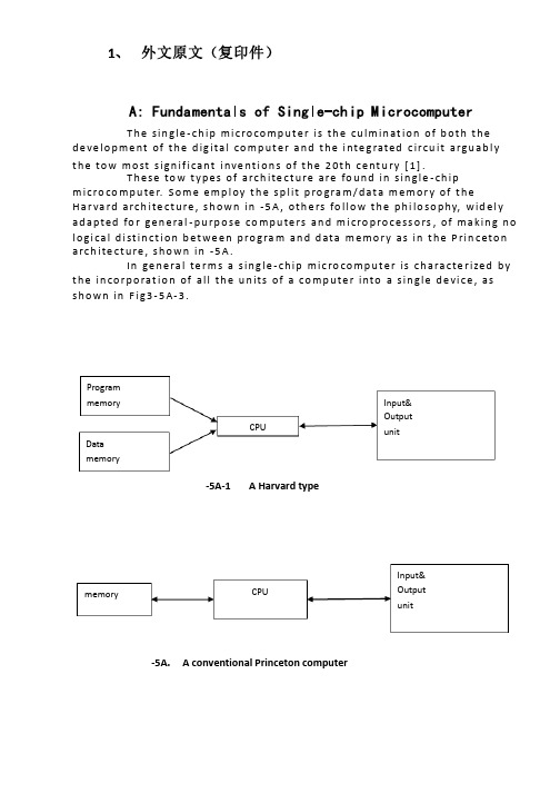
1、 外文原文(复印件)A: Fundamentals of Single-chip MicrocomputerT h e sin gle -ch ip mi c ro co m p u t e r is t h e cu lm in at io n of b ot h t h e d e ve lo p me nt of t h e d ig ita l co m p u t e r a n d t h e i nte g rated c ircu it a rgu ab l y t h e to w mo st s ign if i cant i nve nt i o n s of t h e 20t h c e nt u ry [1].T h ese to w t yp e s of arch ite ct u re are fo u n d in s in gle -ch ip m i cro co m p u te r. S o m e e mp l oy t h e sp l it p ro gra m /d at a m e m o r y of t h e H a r va rd arch ite ct u re , s h o wn in -5A , ot h e rs fo l lo w t h e p h i lo so p hy, wid e l y ad a p ted fo r ge n e ral -p u rp o se co m p u te rs an d m i cro p ro ce ss o rs , of m a kin g n o l o g i ca l d i st in ct i o n b et we e n p ro gra m an d d ata m e m o r y as in t h e P rin c eto n a rch ite ct u re , sh o wn in -5A.In ge n e ra l te r m s a s in g le -ch ip m ic ro co m p u t e r is ch a ra cte r ized b y t h e in co r p o rat io n of all t h e u n its of a co mp u te r into a s in gle d e vi ce , as s h o w n in F i g3-5A-3.-5A-1A Harvard type-5A. A conventional Princeton computerProgrammemory Datamemory CPU Input& Output unitmemoryCPU Input& Output unitResetInterruptsPowerFig3-5A-3. Principal features of a microcomputerRead only memory (ROM).RO M is u su a l l y fo r t h e p e r m an e nt , n o n -vo lat i le sto rage of an ap p l i cat io n s p ro g ram .M a ny m i c ro co m p u te rs a n d m i cro co nt ro l le rs are inte n d ed fo r h i gh -vo lu m e ap p l i cat io n s a n d h e n ce t h e e co n o m i cal man u fa c t u re of t h e d e vi ces re q u ires t h at t h e co nt e nts of t h e p ro gra m me mo r y b e co mm i ed p e r m a n e nt l y d u r in g t h e m a n u fa ct u re of c h ip s . C lea rl y, t h i s imp l ies a r i go ro u s ap p ro a ch to ROM co d e d e ve lo p m e nt s in ce ch an ges can n o t b e mad e af te r m an u fa ct u re .T h i s d e ve l o p m e nt p ro ces s m ay i nvo l ve e mu l at i o n u sin g a so p h ist icated d e ve lo p m e nt syste m wit h a h ard wa re e mu l at i o n capab i l it y as we ll as t h e u s e of p o we rf u l sof t war e to o l s.So m e m an u fa ct u re rs p ro vi d e ad d it i o n a l ROM o p t io n s b y in clu d in g in t h e i r ran ge d e v ic es w it h (o r inte n d ed fo r u s e wit h ) u se r p ro g ram m a b le m e mo r y. T h e s im p lest of t h e se i s u su a l l y d e v i ce wh i ch can o p e rat e in a m i cro p ro ce s so r mo d e b y u s in g s o m e of t h e in p u t /o u t p u t l in es as an ad d res s a n d d ata b u s fo r a cc es sin g exte rn a l m e m o r y. T h is t yp e o f d e vi ce can b e h ave f u n ct i o n al l y as t h e s in gle ch ip m i cro co m p u t e r f ro m wh i ch it i s d e ri ved a lb e it wit h re st r icted I/O an d a m o d if ied exte rn a l c ircu it. T h e u s e of t h e se RO M le ss d e vi ces i s co mmo n e ve n in p ro d u ct io n circu i ts wh e re t h e vo lu m e d o e s n ot ju st if y t h e d e ve lo p m e nt co sts of cu sto m o n -ch ip ROM [2];t h e re ca n st i ll b e a si gn if i cant sav in g in I/O an d o t h e r ch ip s co m pared to a External Timing components System clock Timer/ Counter Serial I/O Prarallel I/O RAM ROMCPUco nve nt io n al m i c ro p ro ces so r b ased circ u it. M o re exa ct re p l a ce m e nt fo rRO M d e v ice s can b e o b tain ed in t h e fo rm of va ria nts w it h 'p i g g y-b a c k'E P ROM(E rasab le p ro gramm ab le ROM )s o cket s o r d e v ice s w it h E P ROMin stead of ROM 。
5G无线通信网络中英文对照外文翻译文献

5G无线通信网络中英文对照外文翻译文献(文档含英文原文和中文翻译)翻译:5G无线通信网络的蜂窝结构和关键技术摘要第四代无线通信系统已经或者即将在许多国家部署。
然而,随着无线移动设备和服务的激增,仍然有一些挑战尤其是4G所不能容纳的,例如像频谱危机和高能量消耗。
无线系统设计师们面临着满足新型无线应用对高数据速率和机动性要求的持续性增长的需求,因此他们已经开始研究被期望于2020年后就能部署的第五代无线系统。
在这篇文章里面,我们提出一个有内门和外门情景之分的潜在的蜂窝结构,并且讨论了多种可行性关于5G无线通信系统的技术,比如大量的MIMO技术,节能通信,认知的广播网络和可见光通信。
面临潜在技术的未知挑战也被讨论了。
介绍信息通信技术(ICT)创新合理的使用对世界经济的提高变得越来越重要。
无线通信网络在全球ICT战略中也许是最挑剔的元素,并且支撑着很多其他的行业,它是世界上成长最快最有活力的行业之一。
欧洲移动天文台(EMO)报道2010年移动通信业总计税收1740亿欧元,从而超过了航空航天业和制药业。
无线技术的发展大大提高了人们在商业运作和社交功能方面通信和生活的能力无线移动通信的显著成就表现在技术创新的快速步伐。
从1991年二代移动通信系统(2G)的初次登场到2001年三代系统(3G)的首次起飞,无线移动网络已经实现了从一个纯粹的技术系统到一个能承载大量多媒体内容网络的转变。
4G无线系统被设计出来用来满足IMT-A技术使用IP面向所有服务的需求。
在4G系统中,先进的无线接口被用于正交频分复用技术(OFDM),多输入多输出系统(MIMO)和链路自适应技术。
4G无线网络可支持数据速率可达1Gb/s的低流度,比如流动局域无线访问,还有速率高达100M/s的高流速,例如像移动访问。
LTE系统和它的延伸系统LTE-A,作为实用的4G系统已经在全球于最近期或不久的将来部署。
然而,每年仍然有戏剧性增长数量的用户支持移动宽频带系统。
外文文献翻译译稿和原文【范本模板】

外文文献翻译译稿1卡尔曼滤波的一个典型实例是从一组有限的,包含噪声的,通过对物体位置的观察序列(可能有偏差)预测出物体的位置的坐标及速度。
在很多工程应用(如雷达、计算机视觉)中都可以找到它的身影。
同时,卡尔曼滤波也是控制理论以及控制系统工程中的一个重要课题。
例如,对于雷达来说,人们感兴趣的是其能够跟踪目标.但目标的位置、速度、加速度的测量值往往在任何时候都有噪声。
卡尔曼滤波利用目标的动态信息,设法去掉噪声的影响,得到一个关于目标位置的好的估计.这个估计可以是对当前目标位置的估计(滤波),也可以是对于将来位置的估计(预测),也可以是对过去位置的估计(插值或平滑).命名[编辑]这种滤波方法以它的发明者鲁道夫。
E。
卡尔曼(Rudolph E. Kalman)命名,但是根据文献可知实际上Peter Swerling在更早之前就提出了一种类似的算法。
斯坦利。
施密特(Stanley Schmidt)首次实现了卡尔曼滤波器。
卡尔曼在NASA埃姆斯研究中心访问时,发现他的方法对于解决阿波罗计划的轨道预测很有用,后来阿波罗飞船的导航电脑便使用了这种滤波器。
关于这种滤波器的论文由Swerling(1958)、Kalman (1960)与Kalman and Bucy(1961)发表。
目前,卡尔曼滤波已经有很多不同的实现.卡尔曼最初提出的形式现在一般称为简单卡尔曼滤波器。
除此以外,还有施密特扩展滤波器、信息滤波器以及很多Bierman, Thornton开发的平方根滤波器的变种.也许最常见的卡尔曼滤波器是锁相环,它在收音机、计算机和几乎任何视频或通讯设备中广泛存在。
以下的讨论需要线性代数以及概率论的一般知识。
卡尔曼滤波建立在线性代数和隐马尔可夫模型(hidden Markov model)上.其基本动态系统可以用一个马尔可夫链表示,该马尔可夫链建立在一个被高斯噪声(即正态分布的噪声)干扰的线性算子上的。
系统的状态可以用一个元素为实数的向量表示.随着离散时间的每一个增加,这个线性算子就会作用在当前状态上,产生一个新的状态,并也会带入一些噪声,同时系统的一些已知的控制器的控制信息也会被加入。
外文翻译原文

Stability of hybrid system limit cycles: application to the compass gait biped RobotIan A. Hiskens'Department of Electrical and Computer EngineeringUniversity of Illinois at Urbana-ChampaignUrbana IL 61801 USAAbstractLimit cycles are common in hybrid systems. However the non-smooth dynamics of such systems makes stability analysis difficult. This paper uses recent extensions of trajectory sensitivity analysis to obtain the characteristic multipliers of non-smooth limit cycles. The stability of a limit cycle is determined by its characteristic multipliers. The concepts are illustrated using a compass gait biped robot example.1 IntroductionHybrid system are characterized by interactions between continuous (smooth) dynamics and discrete events. Such systems are common across a diverse range of application areas. Examples include power systems [l], robotics [2, 3], manufacturing [4] and air-traffic control [5]. In fact, any system where saturation limits are routinely encountered can be thought of as a hybrid system. The limits introduce discrete events which (often) have a significant influence on overall behaviour.Many hybrid systems exhibit periodic behaviour. Discrete events, such as saturation limits, can act to trap the evolving system state within a constrained region of state space. Therefore even when the underlying continuous dynamics are unstable, discrete events may induce a stable limit set. Limit cycles (periodic behaviour) are often created in this way. Other systems, such as robot motion, are naturally periodic.Limit cycles can be stable (attracting), unstable (repelling) or non-stable (saddle). The stability of periodic behaviour is determined by characteristic (or Floquet) multipliers. A periodic solution corresponds to a fixed point of a Poincare map. Stability of the periodic solution is equivalent to stability of the fixed point. The characteristic multipliers are the eigenvalues of the Poincare map linearized about the fixed point. Section 4 reviews the connection between this linearized map and trajectory sensitivities.Poincare maps have been used to analyse the stability of limit cycles in various forms of hybrid systems. However calculation of the underlying trajectory sensitivities has relied upon particular system structures, see for example [7, 8], or numerical differencing, for example [6]. This paper uses a recent generalization of trajectory sensitivity analysis [9] to efficiently detemine the stability of limit cycles in hybrid systems.A hybrid system model is given in Section 2. Section 3 develops the associated variational equations. This is followed in Section 4 by a review of stability analysis of limit cycles. Conclusions and extensions are presented in Section 5.2 ModelDeterministic hybrid systems can be represented by a model that is adapted from a differential-algebraic (DAE) structure. Events are incorporated via impulsive action and switching of algebraic equations, giving the Impulsive Switched (DAIS) modelwheren x R ∈ are dynamic states and my R ∈ are algebraic states;(.)δ is the Dirac delta;(.)u is the unit-step function;,:n mnj f h RR +→;(0)(),:i n mng gR R ±+→; some elements of each(.)gwill usually be identicallyzero, but no elements of the composite g should be identically zero; the()i g± aredefined with the same form as g in (2), resulting in a recursive structure for g;,dey yare selected elements of y that trigger algebraic switching and state reset(impulsive) events respectively;dyandeymay share common elements.The impulse and unit-step terms of the DAIS model can be expressed in alternative forms:Each impulse term of the summation in (1) can be expressed in the state reset formwhere the notation x+denotes the value of x just after the reset event, whilstx-andy-refer to the values of x and y just prior to the event.The contribution of each()i g± in (2) can be expressed aswith (2) becomingThis form is often more intuitive than (2).It can be convenient to establish the partitionswherex -are the continuous dynamic states, for example generator angles, velocities andfluxes;z are discrete dynamic states, such as transformer tap positions and protection relay logic states;λ are parameters such as generator reactances, controller gains and switching times. The partitioning of the differential equations f ensures that away from events,x -evolves according to .(,)x y f x --=, whilst z and λ remain constant. Similarly,the partitioning of the reset equationsjhensures thatx -and λ remain constantat reset events, but the dynamic states z are reset to new values given by(,)jh y x z--+=-. The model can capture complex behaviour, from hysteresis and non-windup limits through to rule-based systems [l]. A more extensive presentation of this model is given in [9].Away from events, system dynamics evolve smoothly according to the familiardifferential-algebraic modelwhere g is composed of(0)gtogether with appropriate choices of()i g- or()i g+ ,depending on the signs of the corresponding elements of yd. At switching events (2),some component equations of g change. To satisfy the new g = 0 equation, algebraic variables y may undergo a step change. Reset events (3) force a discrete change in elements of x. Algebraic variables may also step at a reset event to ensure g= 0 is satisfied with the altered values of x. The flows of and y are defined respectively aswhere x(t) and y(t) satisfy (l),(2), along with initial conditions,3 'Ikajectory SensitivitiesSensitivity of the flowsxφandyφto initial conditionsxare obtained bylinearizing (8),(9) about the nominal trajectory,The time-varying partial derivative matrices given in (12),(13) are known as trajectory sensitiuities, and can be expressed in the alternative formsThe formxx ,xy provides clearer insights into the development of thevariational equations describing the evolution of the sensitivities. The alternative form 0(,)x t x φ, 0(,)yt x φ highlights the connection between the sensitivities and the associated flows. It is shown in Section 4 that these sensitivities underlie the linearization of the Poincare map, and so play a major role in determining the stability of periodic solutions.Away from events, where system dynamics evolve smoothly, trajectory sensitivities 0xx andxy are obtained by differentiating (6),(7) withrespect to 0x.This giveswhere/xf x f≡∂∂, and likewise for the other Jacobian matrices. Note that,,,xyxyf fg gare evaluated along the trajectory, and hence are time varyingmatrices. It is shown in 19, 101 that the numerical solution of this(potentially high order) DAE system can be obtained as a by-product of numerically integrating the original DAE system (6),(7). The extra computational cost is minimal. Initial conditions forxx are obtained from (10) aswhere I is the identity matrix. Initial conditions for 0zy follow directly from(17),Equations (16),(17) describe the evolution of the sensitivitiesxx andxybetween events. However at an event, the sensitivities are generally discontinuous. It is necessary to calculate jump conditions describing the step change inxx andxy . For clarity, consider a single switching/reset event, so the model (1),(2) reduces(effectively) to the formLet ((),()x y ττ) be the point where the trajectory encounters the triggering hypersurface s(x,y) = 0, i.e., the point where an event is initiated. This point is called the junction point and r is the junction time. It is assumed the encounter is transversal.Just prior to event triggering, at time τ-, we haveSimilarly,,y x++are defined for time τ+, just after the event has occurred. It isshown in [9] that the jump conditions for the sensitivitiesxx are given byThe assumption that the trajectory and triggering hypersurface meet transversally ensures a non-zero denominator for 0x τ The sensitivitiesxy . immediatelyafter the event are given byFollowing the event, i.e., for t τ+>, calculation of the sensitivities proceeds according to (16),(17) until the next event is encountered. The jump conditions provide the initial conditions for the post-event calculations.4 Limit Cycle AnalysisStability of limit cycles can be determined using Poincare maps [11, 12]. This section provides a brief review of these concepts, and establishes the connection with trajectory sensitivities.A Poincark map effectively samples the flow of a periodic system once every period. The concept is illustrated in Figure 1. If the limit cycle is stable, oscillations approach the limit cycle over time. The samples provided by the corresponding Poincare map approach a fixed point. A non-stable limit cycle results in divergent oscillations. For such a case the samples of the Poincare map diverge.To define a Poincare map, consider the limit cycle Γshown in Figure 1. Let ∑ be a hyperplane transversal to Γ at*x. The trajectory emanating from*xwill again encounter ∑ at*xafter T seconds, where T is the minimum period of the limit cycle. Due to the continuity of the flowxφwith respect to initial conditions, trajectories starting on ∑ in a neighbourhood of*x. will, in approximately T seconds, intersect ∑ in the vicinity of*x. Hencexφand ∑define a mappingwhere()kT x ττ≈ is the time taken for the trajectory to return to ∑. Complete details can hefound in [11,12]. Stability of the Paincare map (22) is determined by linearizing P at the fixed point*x, i.e.,From the definition of P(z) given by (22), it follows that DP(*x) is closely related to thetrajectory sensitivities***(,)(,)xxT T x x xφφ∂≡∂. In fact, it is shown in [11] thatwhereσ is a vector normal to ∑.The matrix*(,)xT x φis exactly the trajectory sensitivity matrix after one period of the limitcycle, i.e., starting from*xand returning to*x. This matrix is called the Monodromymatrix .It is shown in [11] that for an autonomous system, one eigenvalue of *(,)xT x φ isalways 1, and the corresponding eigenvector lies along **(,)f y x The remaining eigenvalues*(,)xT x φof coincide with the eigenvalues of DP(*x ), and are known as the characteristicmultipliers mi of the periodic solution. The characteristic multipliers are independent of the choice of cross-section ∑ . Therefore, for hybrid systems, it is often convenient to choose ∑ as a triggering hypersurface corresponding to a switching or reset event that occurs along the periodic solution.Because the characteristic multipliers mi are the eigenvalues of the linear map DP(x*), they determine the stability of the Poincarb map P(kx), and hence the stability of the periodic solution.Three cases are of importance: 1. Alli m lie within the unit circle, i.e., 1im<,i ∀.The map is stable, so the periodicsolution is stable. 2. Allim lie outside the unit circle. The periodic solution is unstable.3. Someim lie outside the unit circle. The periodic solution is non-stable.Interestingly, there exists a particular cross-section*∑, such thatwhere *ς∈∑.This cross-section*∑is the hyperplane spanned by the n - 1 eigenvectors of*(,)xT x φthat are not aligned with **(,)f y x . Therefore the vector *σthat is normal to*∑ is the left eigenvector of *(,)xT x φ corresponding to the eigenvalue 1. The hyperplane*∑is invariant under*(,)xT x φ, i.e., **(,)f y x maps vectors *ς∈∑back into*∑.5 ConclusionsHybrid systems frequently exhibit periodic behaviour. However the non-smooth nature of such systems complicates stability analysis. Those complications have been addressed in this paper throughapplication of a generalization of trajectory sensitivity analysis. Deterministic hybrid systems can be represented by a set ofdifferential-algebraic equations, modified to incorporate impulse (state reset) action and constraint switching. The associated variational equations establish jump conditions that describe the evolution of sensitivities through events. These equations provide insights into expansion/contraction effects at events. This is a focus of future research.Standard Poincar6 map results extend naturally to hybrid systems. The Monodromy matrix is obtained by evaluating trajectory sensitivities over one period of the (possibly non-smooth) cyclical behaviour. One eigenvalue of this matrix is always unity. The remaining eigenvalues are the characteristic multipliers of the periodic solution. Stability is ensured if all multipliers lieReferences[l] LA. Hiskens and M.A. Pai, “Hybrid systems view of power system modelling,” in Proceedings of the IEEE International Symposium on Circuits and Systems, Geneva, Switzerland, May 2000.[2] M.H. Raibert, Legged Robots That Balance, MIT Press, Cambridge, MA, 1986.[3] A. Goswami, B. Thuilot, and B. Espiau, “A study of the passive gait of a compass-like biped ro bot: symmetry and chaos,’’ International Journal of Robotics Research, vol. 17, no. 15, 1998.[4] S. Pettersson, “Analysis and design of hybrid systems,” Ph.D. Thesis, Department of Signals and Systems, Chalmers University of Technology, Goteborg, Sweden, 1999.[5] C. Tomlin, G. Pappas, and S. Sastry, “Conflict resolution for air traffic management:A study in multiagent hybrid systems,” IEEE Transactions on Automatic Control, vol. 43, no. 4, pp. 509-521, April 1998.[6] A. Goswami, B. Espiau, and A. Keramane, “Limit cycles in a passive compass gait biped and passivity-mimicking contr ol laws,” Journal of Au tonomous Robots, vol. 4, no. 3, 1997. 171 B.K.H. Wong, H.S.H. Chung, and S.T.S. Lee, ‘Computation of the cycle state-variable sensitivity matrix of PWM DC/DC converters and its applica tion,” IEEE Transactions on Circuit s and Systems I, vol. 47, no. 10, pp. 1542-1548, October 2000.[8] M. Rubensson, B. Lennartsson, and S. Petters son, “Convergence to limit cycles in hybrid systems - an example,” in Prepri nts of 8th International Federation of Automatic Control Symposium on Large Scale Systems: Theo y d Applications, Rio Patras, Greece, 1998, pp. 704-709.[9] I.A. Hiskens and M.A. Pai, “Trajectory sensitivity analysis of hyhrid systems,” IEEE Transactions on Circuits and Systems I, vol. 47, no. 2, pp. 204-220, February 2000.[10]D. Chaniotis, M.A. Pai, and LA. Hiskens, “Sen sitivity analysis of differential-algebraic systems using the GMRES method - Ap plication to power systems,” in Proceedings of the IEEE International Symposium on Circuits and Systems, Sydney, Australia, May 2001.[11]T.S Parker and L.O. Chua, Practical Numerical Algorithms for Chaotic Systems, Springer-Verlag, New York, NY, 1989.[12]R. Seydel, Practical Bifurcation and Stability Analysis, Springer-Verlag. New York, 2nd edition, 1994.。
物流专业外文翻译5
1. The Definition of LogisticsAfter completing a commercial transaction, logistics will execute the transfer of goods from the supplier( seller) to the customer( buyer) in the most cost-effective manner. This is the definition of logistics. During the transfer process, hardware such as logistics facilities and equipment( logistics carriers) are needed, as well as information control and standardization. In addition, supports from the government and logistics association should be in place.Three major functions of logistics(1) Creating time value: same goods can be valued different at different times. Goods often stop during the transfer process, which is professionally called the storage of logistics. It creates the time value for goods.(2) Creating location value: same goods can be valued differently at different locations. The value added during the transfer process is the location value of logistics.(3) Distribution processing value: sometimes logistics create distribution processing value, which changes the length, thickness and packages of the goods. Like popular saying, “ cutting into smaller parts” is the most commonly seen distribution processing within logistics create added value for goods.2. Logistics is a new commercial area, developing from the traditional stage to a modern one. The main differences between these two stage include:(1) Modern logistics adopts containerization techniques. The goods transfer process starts with packaging, followed by transportation, storage and distribution. The whole process is operated under logistics standards. Based on the logistics base module of 600×400mm, from the logistics module of 1,200×1,000mm, and enlarge to the size of2,591×2,438mm-the size of high×wide of the container. It can be adjusted to the standard sizes of containers for trains, trucks and ships.(2) Information technologies are most important for modern logistics. Bar Code, POS, EDI and GPS systems dramatically improve the efficiency and accuracy of the logistics activities. Internet further assists the market development, operation and management of the logistics industry.3.International LogisticsAn increasing number of companies are involving in international markets through exporting, licensing, joins ventures, and ownership. This trend should continue. With such expansion there is a need to develop worldwide logistics networks. Integrated logistics management and cost analysis will be more complex and difficult to manage.There are some future trends in internationalization:(1) More logistics executives with international responsibilities(2) Expansion of the number and size of foreign trade zones.(3) Reduction in the amount of international paperwork and documentation(4) More foreign warehousing is owned and controlled by the exporting firm(5) Increasing number of smaller firm(6) Foreign ownership of logistics service firms, e. g., public warehousing and transportation carriers.(7) Increasing multiple distribution channelsThe international transport and the international logistics are same things in some way. So, when the international trading involved, the firm must establish international logistics systems to provide the products and service demanded. The most significant development in international logistics will be the increasing sophistication information system adopted and independent departments to operate.4.Packaging.Packaging performs two basic functions–marketing and logistics. In marketing the packaging acts promotion and advertising. Its size, weight, color, and printed information attract customers and convey knowledge of the product. When firms are involved in international marketing, packaging becomes even more important. Products sold to foreign countries travel greater distances and undergo more handling operations. The logistics package is to protect the products during the process of logistics.Scrap disposal. The logistics process must effectively and quickly handle, transport, and store waste products. If they can be reused or recycled, logistics company should arrange and move them to the re–production and re–processing locations.Return goods handling. The handling of return goods is often called reverse distribution. Buyers may return items to the seller for a number of reasons. Most logistics systems are not good enough to handle such cases. In many industries, consumers return products for warranty repair, replacement, or recycling, reverse distribution costs may be very high. Reverse distribution will become more important as customers demand more flexible and favorable return policies.5.Third Part Logistics ( TPL)Third Part Logistics provides all the logistics services. They act as a bridge or facilitator between the first part( supplier or producer) and the second part( buyer or customer). The primary objectives of third part logistics providers are to lower the total cost of logistics for the supplier and improve the service level to the customer.Third Part Logistics have been growing rapidly. Cost reduction and demands for batter and cheaper services are the main drives behind the growth. A third part logistics provider will be in a position to consolidate business from several companies and offer frequent pick–ups and deliveries, whereas in–house transportation cannot. Other reasons are as follows:* The company does not specialize in logistics;* The company does not have sufficient resources;* Eager to implement better logistics operation or does not have time to develop the required capabilities in–house;* The company is venturing into a new business with totally different logistics requirements;* Merger or acquisition may make outsourcing logistics operations more attractive than to integrate logistics operations.6.Global LogisticsDeveloped countries often deal with globalization in two ways: to be more cost competitive with third world countries, and to look for new partners in other countries to manufacture components, subassemblies and even the final products. The second approach forces most developed countrie s to get into a new area called “ global logistics”.Benefits of global operations include cheap raw materials and end products, lower labor cost, better quality, increased internal competition and better customer service. Some of the disadvantages are unreliable delivery, poor communication and longer time from design to finish production. Challenges are often cultural and linguistic differences, legal requirements, logistics suppliers or manufacturers, exchange rates.There are three major flows involved in global logistics: material flow, document flow and cash flow.7.Logistics into the FutureLogistics is changing at a rapid and acceleration rate. There are two reasons are its rapid growth:Firstly, pressure to change by the development of the system itself(1) High–speed computing and data transmission can instantly transmit and react to user demand(2) More flexible and accurate logistic planning and control through computers and data processing(3) Flexible computer facilities help problem solving and increase decisions accuracy(4) Awareness of total cost measurement and management accountingSecondly, pressures for changes from the wider economy.(1) Be flexible in handling markets of different sizes for better competition(2) There is increasing specialization in markets and growth in retailing.(3) Life cycles for products are shortening. Logistics systems need to be more efficient, faster and more flexible(4) Move from mass production towards flexible manufacturing system( FMS). These systems enable a company to switch production quickly from one product to another (5) Competitive pressures lead to more efforts to improve customer service.8.The process of logistical integration can be divided into four stages:Stage 1. Began in the early 1960s in the USA and involved the integration of all activities associated with distribution. Separate distribution departments were to coordinate the management of all processes within physical distributionmanagement( PDM).Stage 2. PDM was applied to the inbound movement of materials, components, and subassemblies, generally known as “ materials management”. By the late 1970s, many firms had established “ logistics department” with overall responsibility for the movement, storage, and handling of products upstream and downstream of the production operation.Stage 3. Logistics plays an important coordinating role, as it interfaces with most other functions. With the emergence of business process re–engineering( BPR) in the early 1990s, the relationship between logistics and related functions was redefined.“ System integration” occurred. Cross–functional integration should achieve greater results.物流的定义在完成商业交易之后,物流将以最低成本和最高效益的方式执行将商品从供应商(卖方)流转到顾客(买方)的过程。
- 1、下载文档前请自行甄别文档内容的完整性,平台不提供额外的编辑、内容补充、找答案等附加服务。
- 2、"仅部分预览"的文档,不可在线预览部分如存在完整性等问题,可反馈申请退款(可完整预览的文档不适用该条件!)。
- 3、如文档侵犯您的权益,请联系客服反馈,我们会尽快为您处理(人工客服工作时间:9:00-18:30)。
Contents lists available at ScienceDirect , 2015, 528: 17-24.半正定矩阵的乘积Jianlian Cui , Chi-Kwong Li , Nung-Sing SzeDepartment of Mathematics, Tsinghua University, Beijing 100084, PR China Department of Mathematics, College of William and Mary, Williamsburg,VA 23187, USA Department of Applied Mathematics, The Hong Kong Polytechnic University,Hong Kong摘 要 已知每个具有非负性决定因子的复方阵是正半定矩阵的乘积.在乘积中存在需要两个或五个半正定矩阵的矩阵的表征.然而,缺少乘积中需要三个或四个半正定矩阵的矩阵的表征. 在本文中,我们给出了这两种类型矩阵的完整表征.有了这些结果,我们给了一个确定方阵是否可以表示为k 半正定矩阵的乘积的算法,k = 1,2,3,4,5. 关键词 半正定矩阵,数值范围1 介绍令n M 为n n ⨯个复数矩阵的集合.在[3]中,作者表明,具有非负决定因子的n M 中的矩阵总是可以写成五个或更少的半正定矩阵的乘积.这是对[1]的结果的延伸,n M 中具有的决定因素的每个矩阵都是五个或更少正定矩阵的乘积.类似于[1]中的分析,[3]的作者研究那些可以表示为两个,三个或四个半正定矩阵的乘积.特别地,对于矩阵可以表示为两个半正定矩阵的乘积,也有人表示不是zI 形式的任何矩阵,其中z 不是非负数,可以写成四个半正定矩阵的乘积.此外,[3,定理3.3] 已被证明.如果应用单一相似性来改变方阵形式12*0n T T M T ⎡⎤=∈⎢⎥⎣⎦,使得1T 是可逆的,2T 是零矩阵,并且如果1T 是三个正定矩阵的乘积,则T 可以表示为三个半正定矩阵的乘积.反之并不如此.以下示例显然不是这样.例题1.1让9900T --⎡⎤=⎢⎥⎣⎦,那么9313151132151811T -⎡⎤⎡⎤⎡⎤=⎢⎥⎢⎥⎢⎥-⎣⎦⎣⎦⎣⎦是三个半正定矩阵的乘积. 然而1[9]T =-不是它的乘积三个正定矩阵,因为1det()0T <.当然,可以强制1det()0T >这个明显必要条件推测是否符合额外的假设. 然而,通过修改示例1.12221222322299()()()00II T I A I A I A I --⎡⎤⊗==⊗⊗⊗⎢⎥⎣⎦, 使用因式分解123T A A A =.在修改示例中,我们有129T I =-和220T =.由[1,定理4],129,T I =-是不小于5的正数的乘积确定矩阵.在下一节中,我们将给出可以写为三个半正定矩阵的乘积的矩阵的完整表征,此外,我们添加一个必要和足够的可逆矩阵的条件,可以写成三个正定矩阵的乘积. 通过这些结果,可以使用给定矩阵的Jordan 形式及其数值范围来决定是否可以表示为二,三,四或五个半正定矩阵的乘积.2 三个半正定矩阵的乘积我们将证明以下内容.定理2.1.假设120T R T T ⎡⎤=⎢⎥⎣⎦使得1T 是可逆的. 那么T 是三个半正定矩阵的乘积,当且仅当满足以下条件:2()00.a R T ≠≠或2()0,0,b R T ≠=1T 是三个正定矩阵的乘积. 我们通过一些引理来证明定理2.1引理2.2 令,n A S M ∈,使得S 是可逆的.那么当且仅当 * S AS 是时,A 是奇数个半正定矩阵的乘积.在下一个引理中,我们需要矩阵n A M ∈的数值范围的概念被定义为{}()*:,*1.n W A x Ax x C x x =∈=数值范围是研究矩阵的有用工具. 可以看到[2,第1章]为数值范围的基本属性.引理2.3 假设100p T R T ⎡⎤=⎢⎥⎣⎦使得1m T M ∈是可逆的,并且R 是非零的.那么T 是三个半正定矩阵的乘积.证明:首先,我们表明存在一个p m ⨯矩阵S ,使得1T RS +是三个正定矩阵的乘积.如果1m =,则存在p S C ∈,使得10T RS +>.假设1m >并且R 具有奇异值分解**111k k kR s x y s x y =++,其中1,...,k s s 是非零奇异的R 和1,...,m k x x C ∈和1,..,p k y y C ∈是相应的右和左单位奇异向量. 让{}1,...,m e e 是m C 的标准基.取一个U ,使11Ux e =. 由于1T 是可逆的,所以*11ˆT UTU =也是可逆的. 假设*1ˆt 是1T 的第一行. 令12ˆv t e ε=+,并且1ˆ()T ε是通过用*v 替换其第一行而从1T 获得的m m ⨯矩阵. 取足够小0ε>,使得v 不是1e 的倍数,矩阵1ˆ()T ε仍然是可逆的. 令1*11i S s re y v U θ-=且0r >,[0,2)θπ∈.且****1111ˆ().i U T RS U UTU URSU T re e v θ+=+=+ 由于v 不是1e 的倍数,所以矩阵*1e v 的秩不正常,因此*1()W e v 是具有焦点0和1v0>,其中1v 是v 的第一个条目; 例如,见[2,定理1.3.6]. 由于图()XW X 是连续的,对于足够大的0r >,*11ˆ(/)i W e v e T r θ-+ 仍然包含0作为任何[0,2)θπ∈的内点.那么令**1111ˆˆ()().i i i e W T re e v re W e v T rθθθ-+=+ 此外,可以选择值r 使得11ˆˆdet()/det(())r T T ε>. 现在由行列式相对于第一行的线性度,**111111ˆˆˆdet()det(())det()det()det(())i i T RS U T RS U T re e v T re T θθε+=+=+=+ 因为11ˆˆdet()det(())i T re T θε<,存在[0,2)θπ∈,使得1det()0T RS +>.通过[1,定理3](另见命题2.4),1T RS +是三个正定矩阵的乘积.最后,请注意*1000000mmp p p p T R I T RSR I S T S I I +⎡⎤⎡⎤⎡⎤⎡⎤==⎢⎥⎢⎥⎢⎥⎢⎥⎢⎥⎣⎦⎣⎦⎣⎦⎣⎦ 由[3,定理3.3],T 是三个半正定矩阵的乘积,T 也是引理2.2.定理证明2.1,假设T 是三个半正定矩阵的乘积.如果0R ≠或20T ≠,那么我们完成了.否则,10p T T =⊕是三个半正定矩阵的乘积.由[3,命题3.5],1T 是三个正定矩阵的乘积.为了证明相反,我们考虑以下三种情况.情况1:假设0R ≠我们使用p 上的感应,2T 的大小.如果1p =,则结果从引理2.3得到:2[0]T =. 假设2T 的大小最大为1p -的结果.由于2T 是无效的,不失一般性,我们可以假设2T 是上三角矩阵,2122200T T T ⎡⎤=⎢⎥⎣⎦,其中211p T M -∈. 写12[]R R R =其中1R 是(1)m p ⨯-. 如果10R ≠,矩阵11210T R T ⎡⎤⎢⎥⎣⎦是一种三个半正定矩阵的乘积,例如123PP P . 此外,通过[3,定理2.2](另见命题3.1),我们可以假设12P P 和都是可逆的.令222(1) 1.R X m p T ⎡⎤=+-⨯⎢⎥⎣⎦对于任意的U ,0>ε11312321111*10000000()1P P PP P P P X T P X εεεε----⎡⎤⎡⎤⎡⎤⎡⎤==⎢⎥⎢⎥⎢⎥⎢⎥⎣⎦⎣⎦⎣⎦⎣⎦ 显然,11[0]Q P =⊕和133[]Q P ε-=⊕是半正定矩阵.现在可以选择一个足够小,使0ε>,12121*1()1P P X Q P X εε--⎡⎤=⎢⎥⎣⎦ 也是半正定. 因此,T 是三个半正定矩阵123QQ Q 的乘积.现在假设10R =,那么T 的第() 1m +列是零列. 通过交换第() 1m +和最后一个索引,可以看到T 是排列相似于1212200000T RT T ⎡⎤⎢⎥⎢⎥⎢⎥⎣⎦,其中2122(1),(1)(1),11R m p T p p T p ⨯--⨯-⨯-是是是()还要注意,R 非零,21T 是无效的. 通过归纳,1210T R T ⎡⎤⎢⎥⎣⎦是三个半正定矩阵123PP P 的乘积. 由[3,定理2.2],我们可以进一步假定2P 和3P 都是可逆的. 令220Y T ⎡⎤=⎣⎦,那么任意0ε>,11*1312323211113220000()00000()100T RP P PP P P YP T YYP T εεεε----⎡⎤⎡⎤⎡⎤⎡⎤⎡⎤⎢⎥==⎢⎥⎢⎥⎢⎥⎢⎥⎢⎥⎣⎦⎣⎦⎣⎦⎣⎦⎢⎥⎣⎦再次,可以选择一个足够小的0ε>,使得上述方程左侧的所有三个矩阵都是半正定的. 因此,T 是排列相似的到三个半正定矩阵的乘积,因此T 也可以写成三个半正定矩阵的乘积.情况2:假设 0R =,2T 是非零. 在不失一般性的情况下,我们可以假设2T 是具有零对角线条目的上三角形,而2T 的第一行是非零的.令0mp I S ZI ⎡⎤=⎢⎥⎣⎦,那么 **1*122200000mmp p I T IZ T Z T S TS Z I T I T ⎡⎤⎡⎤⎡⎤⎡⎤==⎢⎥⎢⎥⎢⎥⎢⎥⎢⎥⎣⎦⎣⎦⎣⎦⎣⎦. 情况3:假设 0R =,20T =.如果1T 是三个正定矩阵的乘积,则10p T T =⊕是三个半正定矩阵的乘积.注意,定理2.1取决于检查可逆矩阵是三个正定矩阵的乘积. 这种条件在[1,定理3]中给出. 我们根据以下命题的数值范围重新得出结果,该方法基于[1,定理3和事实3.2]中的讨论.命题2.4 令n T M ∈使得() 0det T >.然后,当且仅当以下之一成立时,T 是三个正定矩阵的乘积.(a )()W T 包含0作为内点.(b )()W T 包含正数, T 的特征值的参数可以被排列成:11-...0nn j j πθθπθ=<≤≤<=∑使得.请注意,在[1,p. 88],作者在条件(3.6b)条件(3.6b)中要求对应于我们的条件(b),T 的所有实际特征值都是正的,这是通过我们假设所有j 的(,)j θππ∈-来保证的.3 确定因素的数量在本节中,我们描述了一种算法,用于确定乘积等于给定的n A M ∈与非负决定子的半正定矩阵的最小数量.我们首先提出以下定理,为矩阵A 的乘积提供一些简单的测试, 两个半正定矩阵满足条件(a),(b),(c)的等价性在[3,定理2.2]中给出.包括一个简短的证明.命题3.1 令A 为方阵. 以下是等同的. (a)A 是两个半正定矩阵的乘积.(b)=A BC ,其中,B C 是半正定矩阵,使得B 或C 是可逆的.(c)A 相似于非负对角矩阵.(d)A 与上部块三角矩阵整体相似,使得对角线块是对应于不同标量的标量矩阵. (e)A 的最小多项式只有简单的非负数. 证明:(c)(d)(e)已是显然.111**11**()():()()()()c b A S DS S S S DS S D S S S -----⇒===()()b a ⇒:显然.()()a c ⇒:假设=A BC ,其中,B C 是n n ⨯半正定. 令U 为酉矩阵,使*00k U BU B =⊕,其中0n k B M -∈为正定矩阵. 让1112*2122CC U CU C C ⎡⎤=⎢⎥⎣⎦. 假设V 是一个整数,使得对于正定矩阵*1100e V C V C =⊕. 我们可以用()U V I ⊕代替U ,并假设1100e C C =⊕.因为C 是半正定的,01*12200000e C C C C C ⎡⎤⎢⎥=⎢⎥⎢⎥⎣⎦,那么 010100**122000000000000000000e e k k k C C CC B B U AU C C ⎡⎤⎡⎤⎡⎤⎡⎤⎢⎥⎢⎥==⎢⎥⎢⎥⎢⎥⎢⎥⎣⎦⎣⎦⎢⎥⎢⎥⎣⎦⎣⎦,11110101012200112200000000000000000000000000000e k k k k k k k e E C C C C EC C B B B E E E E E E C B B ---⎡⎤⎡⎤-⎡⎤⎡⎤⎡⎤⎡⎤⎢⎥⎢⎥⎢⎥⎢⎥⎢⎥⎢⎥⎢⎥⎢⎥⎢⎥⎢⎥⎢⎥⎣⎦⎢⎥⎢⎥⎣⎦⎣⎦⎢⎥⎣⎦⎣⎦⎣⎦⎡⎤=⊕⎢⎥⎣⎦()因此,A 相似于1122000000k e CB B ⎡⎤⊕⎢⎥⎣⎦(,它是半正定的,并且是相似于非负对角矩阵.现在,我们准备提出一个算法来检查具有det ()0,A ≥的矩阵n A M ∈是否可以被写为k 个正半矩阵的乘积,但1,2,3,4,5k ≠.算法3.2 令n A M ∈,det ()0,A ≥如果n A I α=,使得[0,)α∉+∞,则A 可以表示为五个半正定矩阵的乘积.否则,应用与A 的酉矩阵相似得到上三角矩阵120T R T T ⎡⎤=⎢⎥⎣⎦,使得1T 是可逆的,2T 是无效的.(1)如果T 是非负对角矩阵,那么T 本身就是一个半正定矩阵.(2)条件(1)不成立,A 满足命题3.1中的任何一个等效条件. 那么A 可以表示为两个半正定矩阵的乘积.(3)假设(1)和(2)不成立. 那么A 可以表示为三个半正定矩阵的乘积,但不限于以下任何一个.(3.a)R 或2T 不为零.(3.b)0R =和20T =,1T 是三个正定的乘积矩阵.在(3.b)中,如果以下之一成立,则可逆矩阵1T 是三个正定矩阵的乘积. (i)1det 0,T ≠,1()W T 包含0作为内部点,(ii)0不在1()W T 的内部,1()W T 包含正数,j θ∑,其中12k πθθθπ-<≤<⋅⋅⋅<<是1T 的特征值的参数.(4)假设条件(1),(2),(3)不成立,即1=0p T T ⊕,使得上三角矩阵1T 对于(i)和(ii)均不成立,那么A 可以表示为四个半正定矩阵的乘积.4 致谢作者要感谢裁判仔细阅读手稿,崔先生的研究得到了国家自然科学基金委的支持,是滑铁卢大学量子计算研究所的附属成员.他也是上海大学著名教授;他的研究由美国NSF 授权DMS 1331021,西蒙斯基金会赠款351047和中国11571220的NNSF 拨款支持.Sze 的研究得到了香港RGC 授予理大502512及理大中央研究资助G-UC25的支持.5 参考文献[1] C.S. Ballantine, Products of positive definite matrices. IV, Linear Algebra Appl. 3 (1970) 79–114.[2] Horn Johnson, Topics in Matrix Analysis, Cambridge University Press, Cambridge, 1991.[3] P.Y. Wu, Products of positive semidefinite matrices, Linear Algebra Appl. 111 (1988) 53–61.。