Fluent多孔介质英文帮助文件(全)
fluent操作界面中英

fluent操作界面中英文对照Read 读取文件:scheme 方案journal 日志profile 外形Write 保存文件Import:进入另一个运算程序Interpolate:窜改,插入Hardcopy :复制,Batch options 一组选项Save layout 保存设计Grid网格Check 检查Info 报告:size 尺寸;memory usage内存使用情况;zones 区域;partitions划分存储区Polyhedral多面体:Convert domain变换范围Convert skewed cells 变换倾斜的单元Merge 合并Separate 分割Fuse (Merge的意思是将具有相同条件的边界合并成一个;Fuse将两个网格完全贴合的边界融合成内部(interior)来处理,比如叶轮机中,计算多个叶片时,只需生成一个叶片通道网格,其他通过复制后,将重合的周期边界Fuse掉就行了。
注意两个命令均为不可逆操作,在进行操作时注意保存case)Zone 区域:append case file 添加case文档Replace 取代;delete 删除;deactivate使复位;Surface mesh 表面网孔Reordr 追加,添加:Domain 范围;zones区域;Print bandwidth 打印Scale 单位变换Translate 转化Rotate 旋转smooth/swap 光滑/交换Define Models 模型: solver 解算器Pressure based 基于压力Density based 基于密度implicit 隐式, explicit 显示Space 空间:2D,axisymmetric(转动轴),axisymmetric swirl (漩涡转动轴);Time时间:steady 定常,unsteady 非定常Velocity formulation 制定速度:absolute绝对的; relative 相对的Gradient option 梯度选择:以单元作基础;以节点作基础;以单元作梯度的最小正方形。
fluent多孔介质资料搜集
1、多孔介质数值模拟
用fluent计算,多孔介质的数值模拟是怎么设置的?最好详细点,谢谢!
多孔介质模型比较复杂,建议用多孔阶跃模型,后者是前者的二维简化,设置简单,比前者更易用,计算也容易收敛。
只需要设置如下三个参数:
1、face pemeability(面渗透性)
2、Porous Medium Thickness(多孔介质的厚度)
3、Pressure-Jump Coecient(压力阶跃系数)
这三个参数,1、3可以根据压降与速度的函数关系式直接计算得出,比较简单,这里无法弄出公式,就不打了。
2、求教fluent中多孔介质使用的公式应该如何确定?
多孔介质里fluent做了大量简化主要设置孔隙率粘性系数和阻力系数孔隙率由材料提供商直接提供粘性系数和阻力系数可通过压力降与速度降的几组实验得出这在fluent 帮助文件里有说如果不用很精确或没有实验条件可由达西定律近似得出。
追问我看一些例子里有人说要运用udf自定义函数来确定公式,那请问是处理多孔介质问题是都需要运用udf自定义公式?
回答是的如果要精确模拟多孔介质内的情况一定要UDF 。
因为FLUENT中自带的设置模型过于简单所以如果你想得到精确解就一定要UDF 目前很多课题组专门做FLUENT 多孔介质编程方面的研究非常复杂如果你跟本人一样多孔介质只是模拟的一小部分建议还是简化处理不然会相当麻烦。
多孔介质介绍
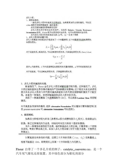
Fluent自带了一个多孔介质的例子,catalytic_converter.cas,是一个汽车尾气催化还原装置,其中绿色部分为催化剂部分其他设置就不说了,只说说与多孔介质有关的设置。
在建立模型时,必须将多孔介质单独划分为一个区域,然后才可以在设置边界条件时将这个区域设置为多孔介质。
1、在zone中选中该区域,在type中选中fluid,点set来到设置面板。
2、在Fluid面板中,选中Porous zone选项,如果忽略多孔区域对湍流的影响,选中Laminar zone。
3、首先是速度方向的设置,在2d中,在direction-1 vector中填入速度方向,在3d中,在direction-1 vector和direction-2 vector中填入速度方向,余下的未填方向,可以根据principal axis得到。
另外也可以用Update From Plane Tool来得到这两个量。
4、填入粘性阻力系数和惯性阻力系数,这两个系数可以通过经验公式得到。
在catalytic_converter.cas中可以看到x方向的阻力系数都比其他两个方向的阻力系数小1000倍,说明x方向是主要的压力降方向,其他两个方向不流通,压力降无限大。
(经验公式可以看帮助文件,其中有详细的介绍)。
随后的Power Law Model 中两个系数是另一种描述压力降的经验模型,一般不使用,可以保留缺省值0。
5、最后是Fluid Porosity,这个值只在模型选择了Physical Velocity 时才起作用,一般对计算没有影响,这个值要小于1。
补充:这个值在计算热传导时也起作用。
下面是改变一些参数后的比较。
1、速度方向的改变:原case:1、0、0 和0、1、0 y=0截面的速度矢量图修正case:-0.7366537、0.06852359、0.6727893 和0.6694272、-0.06727878、0.7398248 y=0速度矢量图2、修改Porosity值为0.5 原case,y=0截面修正case,y=0截面:修正case,且打开solver面板中的Physical Velocity选项:最后比较一下有多孔介质和无多孔介质对流场的影响。
fluent多孔介质简单操作
[转]fluent中多孔介质porous media设置问题
经过痛苦的一段经历,终于将局部问题真相大白,为了使保位同仁不再经过我之痛苦,现在将本人多孔介质经验公布如下,希望各位能加精:
1。
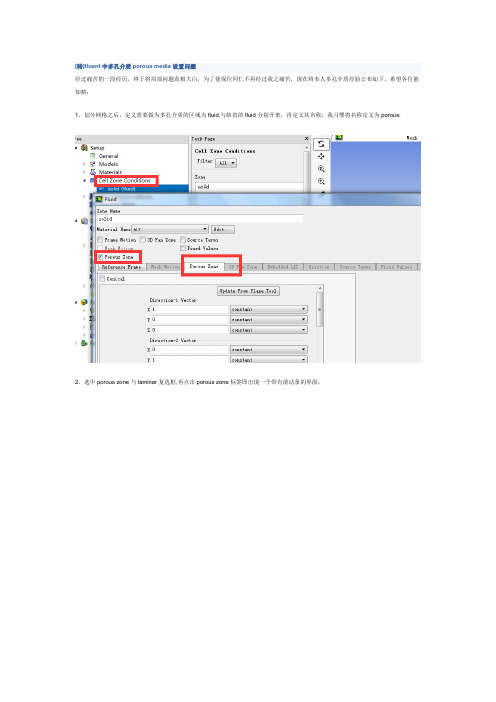
划分网格之后,定义需要做为多孔介质的区域为fluid,与缺省的fluid分别开来,再定义其名称,我习惯将名称定义为porous;
2。
选中porous zone与laminar复选框,再点击porous zone标签即出现一个带有滚动条的界面;
3。
porous zone设置方法:
1)定义矢量:二维定义一个矢量,第二个矢量方向不用定义,是与第一个矢量方向正交的;
三维定义二个矢量,第三个矢量方向不用定义,是与第一、二个矢量方向正交的;
(如何知道矢量的方向:打开grid图,看看X,Y,Z的方向,如果是X向,矢量为1,0,0,同理Y向为0,1,0,Z向为0,0,1,如果所需要的方向与坐标轴正向相反,则定义矢量为负)
圆锥坐标与球坐标请参考fluent帮助。
2)定义粘性阻力1/a与内部阻力C2:请参看本人上一篇博文“终于搞清fluent中多孔粘性阻力与内部阻力的计算方法”,此处不赘述;
3)如果了定义粘性阻力1/a与内部阻力C2,就不用定义C1与C0,因为这是两种不同的定义方法,C1与C0只在幂率模型中出现,该处保持默认就行了;
4)定义孔隙率porousity,默认值1表示全开放,此值按实验测值填写即可。
完了,其他设置与普通k-e或RSM相同。
总结一下,与君共享!。
多孔介质设置及建模实例

我做的多孔介质的简单例子(均为k-e RNG所做))模型仿真结果多孔介质定义的方法(2008-12-14 20:28:12)不知道怎的,这些日子都跟多孔介质干上了1. Define the porous zone.2. Define the porous velocity formulation. (optional)3. Identify the fluid material flowing through the porous medium.4. Enable reactions for the porous zone, if appropriate, and select the reaction mechanism.5. Set the viscous resistance coefficients and the inertial resistance coefficients , and define the direction vectors for which they apply. Alternatively, specify the coefficients for the power-law model.6. Specify the porosity of the porous medium.7. Select the material contained in the porous medium (required only for models that include heat transfer). Note that the specific heat capacity, , for the selected material in the porous zone can only be entered as a constant value.8. Set the volumetric heat generation rate in the solid portion of the porous medium (or any other sources, such as mass or momentum). (optional)9. Set any fixed values for solution variables in the fluid region (optional).10.Suppress the turbulent viscosity in the porous region, if appropriate.11. Specify the rotation axis and/or zone motion, if relevant.fluent中多孔介质porous media设置问题(2008-12-13 20:08:07)标签:杂谈分类:CFD计算流体力学经过痛苦的一段经历,终于将局部问题真相大白,为了使保位同仁不再经过我之痛苦,现在将本人多孔介质经验公布如下,希望各位能加精:1。
fluent多孔介质模型
计算结果
上图为在多孔区内,沿中心线的压强变化。可以看出, 穿过多孔区的压力降约为450Pa.
24
25
△Py, △Pz分别是x,y,z三个方向的压力降。△nx, 别是多孔介质在x,y,z三个方向的真实厚度。
△Px,
△
ny,
△
n z分
7
能量方程的处理
能量方程:
多孔介质对能量方程修正:
对于多孔介质流动,FLUENT仍然解标准能量输运方程,只是修改 了对流项和时间导数项。对对流项的计算采用了有效对流函数,时间 导数项则计入了固体区域对多孔介质的热惯性效应。 多孔区域的有效热传导率keff是由流体的热传导率和固体的热传 导率的体积平均值计算得到:
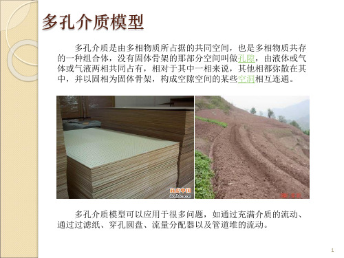
多孔介质模型多孔介质模型多孔介质是由多相物质所占据的共同空间也是多相物质共存的一种组合体没有固体骨架的那部分空间叫做孔隙由液体或气体或气液两相共同占有相对于其中一相来说其他相都弥散在其中并以固相为固体骨架构成空隙空间的某些空洞相互连通
多孔介质模型
多孔介质是由多相物质所占据的共同空间,也是多相物质共存 的一种组合体,没有固体骨架的那部分空间叫做孔隙,由液体或气 体或气液两相共同占有,相对于其中一相来说,其他相都弥散在其 中,并以固相为固体骨架,构成空隙空间的某些空洞相互连通。
14
Fluent中设置
在GAMBIT中将多孔区单独 设置,但其性质仍为fluid.在 fluent的边界条件设置多孔区 的参数,方向设置如下图。多 孔区porous two的粘性阻力设 为1e+10;其余多孔区粘性阻 力设为1e+13,如右边两图所 示。
15
多孔介质的后处理
在多孔介质区域,由于粘性阻力的存在,流体在多孔区内有 较大的压降如第一图所示;porous two的粘性阻力系数是其他多 孔区的千分之一,故流体几乎不会通过porous one和porous three,而全部由porous two通过,如第二图和第三图所示。
Fluent 必备 专业英语

gauge pressure (表压力)mach number (马赫数)X component (X分量)Turbulence Specification Method(湍流指定方法)Turbulence Intensity and Hydraulic Diameter(湍流强度和水利直径)Intensity and viscosity ratio 湍流强度和粘度比Mean Mixture Fraction(平均混合物分数):燃料混合物(包括惰性成分)与氧化剂(包括惰性成分)的质量比Turbulence Length Scale:湍流尺度;Volume Fraction:体积分数;Under-Relaxation Factors:松弛因子;vector:介质,矢量;optical thickness:光学厚度;Second Order Upwind:二阶精度;adiabatic:绝热;Coordinate:坐标Internal Emissivity:内部发射率;Mixture Parameters:混合参数;Slip Velocity:滑动速度;Interaction with Continuous Phase:相互作用的连续相;mean diameter:平均直径;Continuous Phase Iterations:连续相位迭代;Tracking Paramete:追踪主要技术参数;Particle Radiation Interaction:粒子辐射的相互作用;Spread Parameter:传播参数;Stochastic Model:随机模型;Stochastic tracking:随机跟踪;Binary Diffusivity:扩散系数discrete random walk model:离散随机游走模型;thermal conductivity:导热系数;Absorption Coefficient:吸收系数;Injection Properties:射入流属性;Vaporization Temperature:汽化温度;Particle Emissivity:粒子发射;Swelling Coefficient:膨胀系数;normal to boundary:垂直于边界;Granular 粒状FLUENT专业英语【全】Aabort 异常中断, 中途失败, 夭折, 流产, 发育不全,中止计划[任务] accidentally 偶然地, 意外地accretion 增长activation energy 活化能active center 活性中心addition 增加adjacent 相邻的aerosol浮质(气体中的悬浮微粒,如烟,雾等), [化]气溶胶, 气雾剂, 烟雾剂ambient 周围的, 周围环境amines 胺amplitude 广阔, 丰富, 振幅, 物理学名词annular 环流的algebraic stress model(ASM) 代数应力模型algorithm 算法align 排列,使结盟, 使成一行alternately 轮流地analogy 模拟,效仿analytical solution 解析解anisotropic 各向异性的anthracite 无烟煤apparent 显然的, 外观上的,近似的approximation 近似arsenic 砷酸盐assembly 装配associate 联合,联系assume 假设assumption 假设atomization 雾化axial 轴向的Bbattlement 城垛式biography 经历bituminous coal 烟煤blow-off water 排污水blowing devices 鼓风(吹风)装置body force 体积力boiler plant 锅炉装置(车间)Boltzmann 玻耳兹曼Brownian rotation 布朗转动bulk 庞大的bulk density 堆积密度burner assembly 燃烧器组件burnout 燃尽capability 性能,(实际)能力,容量,接受力carbon monoxide COcarbonate 碳酸盐carry-over loss 飞灰损失Cartesian 迪卡尔坐标的casing 箱,壳,套catalisis 催化channeled 有沟的,有缝的char 焦炭、炭circulation circuit 循环回路circumferential velocity 圆周速度clinkering 熔渣clipped 截尾的clipped Gaussian distribution 截尾高斯分布closure (模型的)封闭cloud of particles 颗粒云cluster 颗粒团coal off-gas 煤的挥发气体coarse 粗糙的coarse grid 疏网格,粗网格coaxial 同轴的coefficient of restitution 回弹系数;恢复系数coke 碳collision 碰撞competence 能力competing process 同时发生影响的competing-reactions submodel 平行反应子模型component 部分分量composition 成分cone shape 圆锥体形状configuration 布置,构造confined flames 有界燃烧confirmation 证实, 确认, 批准conservation 守恒不灭conservation equation 守恒方程conserved scalars 守恒标量considerably 相当地consume 消耗contact angle 接触角contamination 污染contingency 偶然, 可能性, 意外事故, 可能发生的附带事件continuum 连续体converged 收敛的conveyer 输运机convolve 卷cooling wall 水冷壁correlation 关联(式)correlation function 相关函数corrosion 腐蚀,锈coupling 联结, 接合, 耦合crack 裂缝,裂纹creep up (水)渗上来,蠕升critical 临界critically 精密地cross-correlation 互关联cumulative 累积的curtain wall 护墙,幕墙curve 曲线custom 习惯, 风俗, <动词单用>海关, (封建制度下)定期服劳役, 缴纳租税, 自定义, <偶用作>关税v.定制, 承接定做活的cyano 氰(基),深蓝,青色cyclone 旋风子,旋风,旋风筒cyclone separator 旋风分离器[除尘器]cylindrical 柱坐标的cylindrical coordinate 柱坐标dead zones 死区decompose 分解decouple 解藕的defy 使成为不可能demography 统计deposition 沉积derivative with respect to 对…的导数derivation 引出, 来历, 出处, (语言)语源, 词源design cycle 设计流程desposit 积灰,结垢deterministic approach 确定轨道模型deterministic 宿命的deviation 偏差devoid 缺乏devolatilization 析出挥发分,液化作用diffusion 扩散diffusivity 扩散系数digonal 二角(的), 对角的,二维的dilute 稀的diminish 减少direct numerical simulation 直接数值模拟discharge 释放discrete 离散的discrete phase 分散相, 不连续相discretization [数]离散化deselect 取消选定dispersion 弥散dissector 扩流锥dissociate thermally 热分解dissociation 分裂dissipation 消散, 分散, 挥霍, 浪费, 消遣, 放荡, 狂饮distribution of air 布风divide 除以dot line 虚线drag coefficient 牵引系数,阻力系数drag and drop 拖放drag force 曳力drift velocity 漂移速度driving force 驱[传, 主]动力droplet 液滴drum 锅筒dry-bottom-furnace 固态排渣炉dry-bottom 冷灰斗,固态排渣duct 管dump 渣坑dust-air mixture 一次风EBU---Eddy break up 漩涡破碎模型eddy 涡旋effluent 废气,流出物elastic 弹性的electro-staic precipitators 静电除尘器emanate 散发, 发出, 发源,[罕]发散, 放射embrasure 喷口,枪眼emissivity [物]发射率empirical 经验的endothermic reaction 吸热反应enhance 增,涨enlarge 扩大ensemble 组,群,全体enthalpy 焓entity 实体entrain 携带,夹带entrained-bed 携带床equilibrate 保持平衡equilibrium 化学平衡ESCIMO-----Engulfment(卷吞) Stretching(拉伸) Coherence(粘附) In terdiffusion-interaction(相互扩散和化学反应) Moving-observer(运动观察者)exhaust 用尽, 耗尽, 抽完, 使精疲力尽排气排气装置用不完的, 不会枯竭的exit 出口,排气管exothermic reaction 放热反应expenditure 支出,经费expertise 经验explicitly 明白地, 明确地extinction 熄灭的extract 抽出,提取evaluation 评价,估计,赋值evaporation 蒸发(作用)Eulerian approach 欧拉法facilitate 推动,促进factor 把…分解fast chemistry 快速化学反应fate 天数, 命运, 运气,注定, 送命,最终结果feasible 可行的,可能的feed pump 给水泵feedstock 填料fine grid 密网格,细网格finite difference approximation 有限差分法flamelet 小火焰单元flame stability 火焰稳定性flow pattern 流型fluctuating velocity 脉动速度fluctuation 脉动,波动flue 烟道(气)flue duck 烟道fluoride 氟化物fold 夹层块forced-and-induced draft fan 鼓引风机forestall 防止fouling 沾污fraction 碎片部分,百分比fragmentation 破碎fuel-lean flamefuel-rich regions 富燃料区,浓燃料区fuse 熔化,熔融gas duct 烟道gas-tight 烟气密封gasification 气化(作用)gasifier 气化器generalized model 通用模型Gibbs function Method 吉布斯函数法Gordon 戈登governing equation 控制方程gradient 梯度graphics 图gross efficiency 总效率hazard 危险header 联箱helically 螺旋形地heterogeneous 异相的heat flux 热流(密度)heat regeneration 再热器heat retention coeff 保热系数histogram 柱状图homogeneous 同相的、均相的hopper 漏斗horizontally 卧式的,水平的hydrodynamic drag 流体动力阻力hydrostatic pressure 静压hypothesis 假设humidity 湿气,湿度,水分含量identical 同一的,完全相同的ignition 着火illustrate 图解,插图in common with 和…一样in excess of 超过, 较...为多in recognition of 承认…而,按照in terms of 根据, 按照, 用...的话, 在...方面incandescent 白炽的,光亮的inception 起初induced-draft fan 强制引风机inert 无活动的, 惰性的, 迟钝的inert atmosphere 惰性气氛inertia 惯性, 惯量inflammability 可燃性injection 引入,吸引inleakage 漏风量inlet 入口inlet vent 入烟口instantaneous reaction rate 瞬时反应速率instantaneous velocity 瞬时速度instruction 指示, 用法说明(书), 教育, 指导, 指令intake fan 进气风扇integral time 积分时间integration 积分interface 接触面intermediate 中间的,介质intermediate species 中间组分intermittency model of turbulence 湍流间歇模型intermixing 混合intersect 横断,相交interval 间隔intrinsic 内在的inverse proportion 反比irreverse 不可逆的irreversible 不可逆的,单向的isothermal 等温的, 等温线的,等温线isotropic 各向同性的joint 连接justify 认为Kelvin 绝对温度,开氏温度kinematic viscosity 动粘滞率, 动粘度kinetics 动力学Lagrangian approach 拉格朗日法laminarization 层流化的Laminar 层流Laminar Flamelet Concept 层流小火焰概念large-eddy simulation (LES) 大涡模拟leak 泄漏length scale 湍流长度尺度liberate 释放lifetime 持续时间,(使用)寿命,使用期literature 文学(作品), 文艺, 著作, 文献lining 炉衬localized 狭小的logarithm [数] 对数Low Reynolds Number Modeling Method 低雷诺数模型macropore 大孔隙(直径大于1000埃的孔隙)manipulation 处理, 操作, 操纵, 被操纵mass action 质量作用mass flowrate 质量流率Mcbride 麦克布利德mean free paths 平均自由行程mean velocity 平均速度meaningful 意味深长的,有意义的medium 均匀介质mercury porosimetery 水银测孔计, 水银孔率计mill 磨碎,碾碎mineral matter 矿物质mixture fraction 混合分数modal 众数的,形式的, 样式的, 形态上的, 情态的, 语气的[计](对话框等)模式的modulus 系数, 模数moisture 水分,潮湿度molar 质量的, [化][物]摩尔的moment 力矩,矩,动差momentum 动量momentum transfer 动量传递monobloc 单元机组monobloc units 单组mortar 泥灰浆mount 安装,衬底Monte Carlo methods 蒙特卡罗法multiflux radiation model 多(4/6)通量模型multivariate [统][数]多变量的,多元的negative 负Newton-Rephson 牛顿—雷夫森nitric oxide NO2node 节点non-linear 非线性的numerical control 数字控制numerical simulation 数值模拟table look-up scheme 查表法tabulate 列表tangential 切向的tangentially 切线tilting 摆动the heat power of furnace 热负荷the state-of-the-art 现状thermal effect 反应热thermodynamic 热力学thermophoresis 热迁移,热泳threshold 开始, 开端, 极限tortuosity 扭转, 曲折, 弯曲toxic 有毒的,毒的trajectory 轨迹,弹道tracer 追踪者, 描图者, (铁笔等)绘图工具translatory 平移的transport coefficients 输运系数transverse 横向,横线triatomic 三原子的turbulence intensity 湍流强度turbulent 湍流turbulent burner 旋流燃烧器turbulization 涡流turnaround 完成two-scroll burner 双涡流燃烧器unimodal [统](频率曲线或分布)单峰的,(现象或性质) 用单峰分布描述的validate 使…证实validation 验证vaporization 汽化Variable 变量variance 方差variant 不同的,变量variation 变更, 变化, 变异, 变种, [音]变奏, 变调vertical 垂直的virtual mass 虚质量viscosity 粘度visualization 可视化volatile 易挥发性的volume fraction 体积分数, 体积分率, 容积率volume heat 容积热vortex burner 旋流式燃烧器vorticity 旋量wall-function method 壁面函数法water equivalent 水当量weighting factor 权重因数unity (数学)一uniform 不均匀unrealistic 不切实际的, 不现实的Zeldovich 氮的氧化成一氧化氮的过程zero mean 零平均值zone method 区域法。
Fluent计算多孔介质模型资料
广东省深圳市宝安区沙井辛养社区西部工业园 TEL:+86-755-3366-8888 FAX:+86-755-3366-0612Fluent计算多孔介质模型资料这是一个多孔介质例子,进口速度为0.01m/s,组份为液态水和氧气,其中氧气从多孔介质porous jump 渗透过去,如何看氧气在tissue中扩散的。
porous jump的face permeability1 a=e-8 m_2thickness 设为0.0001pressure jump coefficient为默认porous zone设置如下:direction vector 1, 1,viscous resistance 100 eachinertial resistance 100 eachporosity 0.1边界条件设置如下:Ab – wall - defaultBc – wall – defaultBe – porous jump – face permeability 1e-8, porous medium thickness0.0001Cd – outflow rating – 0.5De – wall – defaultDefault interior – interiorDefault interior001 – interiorDefault interior019 – interiorEf – wall - defaultFg – outflow rating – 1Fluid - porous zone - direction vector 1, 1, viscous resistance 100 each,inertial resistance 100 each, porosity 0.1Gh- wall - defaultHi – wall - defaultHk - porous jump same conditions as otherIj – outflow – 0.5Jk – wall – defaultKl – wall – defaultLa – velocity inlet – 0.01 m/s, temperature 300K, 0.5 mass fraction O2 Lfluid – porous zone - direction vector 1, 1, viscous resistance 100 each,inertial resistance 100 each, porosity 0.1Pipefluid – fluid – default (no porous zone)Models – species transport – water and oxygen mixtureVariations – different boundary conditions at top and bottom (outflow, wall ect)注意,其中porous zone在gambit中设置为fluid,在fluent中设置为porous zone边界条件设置如下:Ab – wall - defaultBc – wall – defaultBe – porous jump – face permeability 1e-8, porous medium thickness0.0001Cd – outflow rating – 0.5De – wall – defaultDefault interior – interiorDefault interior001 – interiorDefault interior019 – interiorEf – wall - defaultFg – outflow rating – 1Fluid - porous zone - direction vector 1, 1, viscous resistance 100 each,inertial resistance 100 each, porosity 0.1Gh- wall - defaultHi – wall - defaultHk - porous jump same conditions as otherIj – outflow – 0.5Jk – wall – defaultKl – wall – defaultLa – velocity inlet – 0.01 m/s, temperature 300K, 0.5 mass fraction O2 Lfluid – porous zone - direction vector 1, 1, viscous resistance 100 each,inertial resistance 100 each, porosity 0.1Pipefluid – fluid – default (no porous zone)Models – species transport – water and oxygen mixtureVariations – different boundary conditions at top and bottom (outflow, wall ect) 注意,其中porous zone在gambit中设置为fluid,在fluent中设置为porous zone。
- 1、下载文档前请自行甄别文档内容的完整性,平台不提供额外的编辑、内容补充、找答案等附加服务。
- 2、"仅部分预览"的文档,不可在线预览部分如存在完整性等问题,可反馈申请退款(可完整预览的文档不适用该条件!)。
- 3、如文档侵犯您的权益,请联系客服反馈,我们会尽快为您处理(人工客服工作时间:9:00-18:30)。
7.19 Porous Media ConditionsThe porous media model can be used for a wide variety of problems, including flows through packed beds, filter papers, perforated plates, flow distributors, and tube banks. When you use this model, you define a cell zone in which the porous media model is applied and the pressure loss in the flow is determined via your inputs as described in Section 7.19.2. Heat transfer through the medium can also be represented, subject to the assumption of thermal equilibrium between the medium and the fluid flow, as described in Section 7.19.3.A 1D simplification of the porous media model, termed the "porous jump,'' can be used to model a thin membrane with known velocity/pressure-drop characteristics. The porous jump model is applied to a face zone, not to a cell zone, and should be used (instead of the full porous media model) whenever possible because it is more robust and yields better convergence. See Section 7.22 for details.7.19.1 Limitations and Assumptions of the Porous Media ModelThe porous media model incorporates an empirically determined flow resistance in a region of your model defined as "porous''. In essence, the porous media model is nothing more than an added momentum sink in the governing momentum equations. As such, the following modeling assumptions and limitations should be readily recognized:•Since the volume blockage that is physically present is not represented in the model, by default FLUENT uses and reports asuperficial velocity inside the porous medium, based on thevolumetric flow rate, to ensure continuity of the velocity vectorsacross the porous medium interface. As a more accurate alternative,you can instruct FLUENT to use the true (physical) velocity inside the porous medium. See Section 7.19.7 for details.•The effect of the porous medium on the turbulence field is only approximated. See Section 7.19.4 for details.•When applying the porous media model in a moving reference frame, FLUENT will either apply the relative reference frame or the absolute reference frame when you enable the Relative VelocityResistance Formulation. This allows for the correct prediction of the source terms. For more information about porous media, seeSections 7.19.6 and 7.19.6.•When specifying the specific heat capacity,P C, for the selected material in the porous zone,C must be entered as a constant value.P•7.19.2 Momentum Equations for Porous Media •Porous media are modeled by the addition of a momentum source term to the standard fluid flow equations. The source term iscomposed of two parts: a viscous loss term (Darcy, the first term on the right-hand side of Equation 7.19-1 ) , and an inertial loss term(the second term on the right-hand side of Equation 7.19-1)(7.19-1)•where is the source term for the th ( , , or ) momentum equation, is the magnitude of the velocity and and areprescribed matrices. This momentum sink contributes to the pressure gradient in the porous cell, creating a pressure drop that isproportional to the fluid velocity (or velocity squared) in the cell. •To recover the case of simple homogeneous porous media(7.19-2)where is the permeability and is the inertial resistance factor, simply specify and as diagonal matrices with and , respectively, on the diagonals (and zero for the other elements).•FLUENT also allows the source term to be modeled as a power law of the velocity magnitude:(7.19-3)•where and are user-defined empirical coefficients.In the power-law model, the pressure drop is isotropic and theunits for are SI.Darcy's Law in Porous Media••In laminar flows through porous media, the pressure drop is typically proportional to velocity and the constant can be considered to bezero. Ignoring convective acceleration and diffusion, the porousmedia model then reduces to Darcy's Law:•(7.19-4)••The pressure drop that FLUENT computes in each of the three ( , , ) coordinate directions within the porous region is then ••••(7.19-5)•••••where are the entries in the matrix inEquation 7.19-1, are the velocity components in the , ,and directions, and , , and are the thicknesses of the medium in the , , and directions.•Here, the thickness of the medium ( , , or ) is the actual thickness of the porous region in your model. Thus if the thicknesses used in your model differ from the actual thicknesses, you must make the adjustments in your inputs for .•Inertial Losses in Porous Media••At high flow velocities, the constant in Equation 7.19-1 providesa correction for inertial losses in the porous medium. This constantcan be viewed as a loss coefficient per unit length along the flowdirection, thereby allowing the pressure drop to be specified as afunction of dynamic head.•If you are modeling a perforated plate or tube bank, you can sometimes eliminate the permeability term and use the inertial loss term alone, yielding the following simplified form of the porousmedia equation:•(7.19-6)••or when written in terms of the pressure drop inthe , , directions:•(7.19-7) ••Again, the thickness of the medium ( , , or ) is the thickness you have defined in your model.•7.19.3 Treatment of the Energy Equation in Porous Media•FLUENT solves the standard energy transport equation (Equation 13.2-1) in porous media regions with modifications to the conduction flux and the transient terms only. In the porous medium, the conduction flux uses an effective conductivity and the transient term includes the thermal inertia of the solid region on the medium:•(7.19-8)••where•= total fluid energy= total solid medium energy= porosity of the medium= effective thermal conductivity of the medium= fluid enthalpy source term••Effective Conductivity in the Porous Medium••The effective thermal conductivity in the porous medium, , is computed by FLUENT as the volume average of the fluidconductivity and the solid conductivity:•(7.19-9)••where•= porosity of the medium= fluid phase thermal conductivity (including the turbulent contribution, )= solid medium thermal conductivity••The fluid thermal conductivity and the solid thermalconductivity can be computed via user-defined functions.•The anisotropic effective thermal conductivity can also be specified via user-defined functions. In this case, the isotropic contributionsfrom the fluid, , are added to the diagonal elements of the solidanisotropic thermal conductivity matrix.7.19.4 Treatment of Turbulence in Porous MediaFLUENT will, by default, solve the standard conservation equations for turbulence quantities in the porous medium. In this default approach, turbulence in the medium is treated as though the solid medium has no effect on the turbulence generation or dissipation rates. This assumption may be reasonable if the medium's permeability is quite large and the geometric scale of the medium does not interact with the scale of the turbulent eddies. In other instances, however, you may want to suppress the effect of turbulence in the medium.If you are using one of the turbulence models (with the exception of the Large Eddy Simulation (LES) model), you can suppress the effect of turbulence in a porous region by setting the turbulent contribution to viscosity, , equal to zero. When you choose this option, FLUENT will transport the inlet turbulence quantities through the medium, but their effect on the fluid mixing and momentum will be ignored. In addition, the generation of turbulence will be set to zero in the medium. This modeling strategy is enabled by turning on the Laminar Zone option inthe Fluid panel. Enabling this option implies that is zero and that generation of turbulence will be zero in this porous zone. Disabling the option (the default) implies that turbulence will be computed in the porous region just as in the bulk fluid flow. Refer to Section 7.17.1 for details about using the Laminar Zone option.7.19.5 Effect of Porosity on Transient Scalar EquationsFor transient porous media calculations, the effect of porosity on thetime-derivative terms is accounted for in all scalar transport equations andthe continuity equation. When the effect of porosity is taken into account, the time-derivative term becomes , where is the scalar quantity ( , , etc.) and is the porosity.The effect of porosity is enabled automatically for transient calculations, and the porosity is set to 1 by default.7.19.6 User Inputs for Porous MediaWhen you are modeling a porous region, the only additional inputs for the problem setup are as follows. Optional inputs are indicated as such.1. Define the porous zone.2. Define the porous velocity formulation. (optional)3. Identify the fluid material flowing through the porous medium.4. Enable reactions for the porous zone, if appropriate, and select the reaction mechanism.5. Enable the Relative Velocity Resistance Formulation. By default, this option is already enabled and takes the moving porous media into consideration (as described in Section 7.19.6).6. Set the viscous resistance coefficients ( in Equation7.19-1,or in Equation 7.19-2) and the inertial resistance coefficients ( in Equation 7.19-1, or in Equation 7.19-2), and define the direction vectors for which they apply. Alternatively, specify the coefficients for the power-law model.7. Specify the porosity of the porous medium.8. Select the material contained in the porous medium (required only for models that include heat transfer). Note that the specific heat capacity, , for the selected material in the porous zone can only be entered as a constant value.9. Set the volumetric heat generation rate in the solid portion of the porous medium (or any other sources, such as mass or momentum). (optional) 10. Set any fixed values for solution variables in the fluid region (optional).11. Suppress the turbulent viscosity in the porous region, if appropriate.12. Specify the rotation axis and/or zone motion, if relevant.Methods for determining the resistance coefficients and/or permeability are presented below. If you choose to use the power-law approximation of the porous-media momentum source term, you will enter thecoefficients and in Equation 7.19-3 instead of the resistance coefficients and flow direction.You will set all parameters for the porous medium inFigure 7.19.1:The Fluid Panel for a Porous Zone Defining the Porous ZoneAs mentioned in Section 7.1, a porous zone is modeled as a special type of fluid zone. To indicate that the fluid zone is a porous region, enablethe Porous Zone option in the Fluid panel. The panel will expand to show the porous media inputs (as shown in Figure 7.19.1).Defining the Porous Velocity FormulationThe Solver panel contains a Porous Formulation region where you can instruct FLUENT to use either a superficial or physical velocity in the porous medium simulation. By default, the velocity is set to Superficial Velocity. For details about using the Physical Velocity formulation, see Section 7.19.7.Defining the Fluid Passing Through the Porous MediumTo define the fluid that passes through the porous medium, select the appropriate fluid in the Material Name drop-down list in the Fluid panel. If you want to check or modify the properties of the selected material, you can click Edit... to open the Material panel; this panel contains just the properties of the selected material, not the full contents of thestandard Materials panel.If you are modeling species transport or multiphase flow,the Material Name list will not appear in the Fluid panel.For species calculations, the mixture material for allfluid/porous zones will be the material you specified inthe Species Model panel. For multiphase flows, the materialsare specified when you define the phases, as described inSection 23.10.3.Enabling Reactions in a Porous ZoneIf you are modeling species transport with reactions, you can enable reactions in a porous zone by turning on the Reaction option inthe Fluid panel and selecting a mechanism in the ReactionMechanism drop-down list.If your mechanism contains wall surface reactions, you will also need to specify a value for the Surface-to-Volume Ratio. This value is the surfacearea of the pore walls per unit volume ( ), and can be thought of as a measure of catalyst loading. With this value, FLUENT can calculate the total surface area on which the reaction takes place in each cell bymultiplying by the volume of the cell. See Section 14.1.4 for details about defining reaction mechanisms. See Section 14.2for details about wall surface reactions.Including the Relative Velocity Resistance FormulationPrior to FLUENT 6.3, cases with moving reference frames used the absolute velocities in the source calculations for inertial and viscous resistance. This approach has been enhanced so that relative velocities are used for the porous source calculations (Section 7.19.2). Using the Relative Velocity Resistance Formulation option (turned on by default) allows you to better predict the source terms for cases involving moving meshes or moving reference frames (MRF). This option works well in cases withnon-moving and moving porous media. Note that FLUENT will use the appropriate velocities (relative or absolute), depending on your case setup. Defining the Viscous and Inertial Resistance CoefficientsThe viscous and inertial resistance coefficients are both defined in the same manner. The basic approach for defining the coefficients using a Cartesian coordinate system is to define one direction vector in 2D or two direction vectors in 3D, and then specify the viscous and/or inertial resistance coefficients in each direction. In 2D, the second direction, which is not explicitly defined, is normal to the plane defined by the specified direction vector and the direction vector. In 3D, the third direction is normal to the plane defined by the two specified direction vectors. For a 3D problem, the second direction must be normal to the first. If you fail to specify two normal directions, the solver will ensure that they are normal by ignoringany component of the second direction that is in the first direction. You should therefore be certain that the first direction is correctly specified.You can also define the viscous and/or inertial resistance coefficients in each direction using a user-defined function (UDF). The user-defined options become available in the corresponding drop-down list when the UDF has been created and loaded into FLUENT. Note that the coefficients defined in the UDF must utilize the DEFINE_PROFILE macro. For more information on creating and using user-defined function, see the separate UDF Manual.If you are modeling axisymmetric swirling flows, you can specify an additional direction component for the viscous and/or inertial resistance coefficients. This direction component is always tangential to the other two specified directions. This option is available for both density-based and pressure-based solvers.In 3D, it is also possible to define the coefficients using a conical (or cylindrical) coordinate system, as described below.Note that the viscous and inertial resistance coefficients aregenerally based on the superficial velocity of the fluid in theporous media.The procedure for defining resistance coefficients is as follows:1. Define the direction vectors.•To use a Cartesian coordinate system, simply specify the Direction-1 Vector and, for 3D, the Direction-2 Vector. The unspecifieddirection will be determined as described above. These directionvectors correspond to the principle axes of the porous media.For some problems in which the principal axes of the porous mediumare not aligned with the coordinate axes of the domain, you may notknow a priori the direction vectors of the porous medium. In suchcases, the plane tool in 3D (or the line tool in 2D) can help you todetermine these direction vectors.(a) "Snap'' the plane tool (or the line tool) onto the boundary of theporous region. (Follow the instructions inSection 27.6.1 or 27.5.1 for initializing the tool to a position on anexisting surface.)(b) Rotate the axes of the tool appropriately until they are alignedwith the porous medium.(c) Once the axes are aligned, click on the Update From PlaneTool or Update From Line Tool button inthe Fluid panel. FLUENT will automatically set the Direction-1Vector to the direction of the red arrow of the tool, and (in 3D)the Direction-2 Vector to the direction of the green arrow.•To use a conical coordinate system (e.g., for an annular, conical filter element), follow the steps below. This option is available only in 3D cases.(a) Turn on the Conical option.(b) Specify the Cone Axis Vector and Point on Cone Axis. Thecone axis is specified as being in the direction of the Cone AxisVector (unit vector), and passing through the Point on Cone Axis.The cone axis may or may not pass through the origin of thecoordinate system.(c) Set the Cone Half Angle (the angle between the cone's axis andits surface, shown in Figure 7.19.2). To use a cylindrical coordinate system, set the Cone Half Angle to 0.Figure 7.19.2:Cone Half AngleFor some problems in which the axis of the conical filter element is not aligned with the coordinate axes of the domain, you may notknow a priori the direction vector of the cone axis and coordinates ofa point on the cone axis. In such cases, the plane tool can help you todetermine the cone axis vector and point coordinates. One method is as follows:(a) Select a boundary zone of the conical filter element that isnormal to the cone axis vector in the drop-down list next to the Snap to Zone button.(b) Click on the Snap to Zone button. FLUENT will automatically"snap'' the plane tool onto the boundary. It will also set the Cone Axis Vector and the Point on Cone Axis. (Note that you will still have to set the Cone Half Angle yourself.)An alternate method is as follows:(a) "Snap'' the plane tool onto the boundary of the porous region.(Follow the instructions in Section 27.6.1 for initializing the tool to aposition on an existing surface.)(b) Rotate and translate the axes of the tool appropriately until thered arrow of the tool is pointing in the direction of the cone axisvector and the origin of the tool is on the cone axis.(c) Once the axes and origin of the tool are aligned, click onthe Update From Plane Tool button inthe Fluid panel. FLUENT will automatically set the Cone AxisVector and the Point on Cone Axis. (Note that you will still have toset the Cone Half Angle yourself.)2. Under Viscous Resistance, specify the viscous resistancecoefficient in each direction.Under Inertial Resistance, specify the inertial resistance coefficient in each direction. (You will need to scroll down with the scroll bar to view these inputs.)For porous media cases containing highly anisotropic inertial resistances, enable Alternative Formulation under Inertial Resistance.The Alternative Formulation option provides better stability to the calculation when your porous medium is anisotropic. The pressure loss through the medium depends on the magnitude of the velocity vector ofthe i th component in the medium. Using the formulation ofEquation 7.19-6 yields the expression below:(7.19-10) Whether or not you use the Alternative Formulation option depends on how well you can fit your experimentally determined pressure drop data to the FLUENT model. For example, if the flow through the medium is aligned with the grid in your FLUENT model, then it will not make a difference whether or not you use the formulation.For more infomation about simulations involving highly anisotropic porous media, see Section 7.19.8.Note that the alternative formulation is compatible only withthe pressure-based solver.If you are using the Conical specification method, Direction-1 is the cone axis direction, Direction-2 is the normal to the cone surface (radial ( ) direction for a cylinder), and Direction-3 is the circumferential ( ) direction.In 3D there are three possible categories of coefficients, and in 2D there are two:•In the isotropic case, the resistance coefficients in all directions are the same (e.g., a sponge). For an isotropic case, you must explicitlyset the resistance coefficients in each direction to the same value.•When (in 3D) the coefficients in two directions are the same and those in the third direction are different or (in 2D) the coefficients inthe two directions are different, you must be careful to specify thecoefficients properly for each direction. For example, if you had aporous region consisting of cylindrical straws with small holes inthem positioned parallel to the flow direction, the flow would passeasily through the straws, but the flow in the other two directions(through the small holes) would be very little. If you had a plane offlat plates perpendicular to the flow direction, the flow would notpass through them at all; it would instead move in the other twodirections.•In 3D the third possible case is one in which all three coefficients are different. For example, if the porous region consisted of a plane ofirregularly-spaced objects (e.g., pins), the movement of flow betweenthe blockages would be different in each direction. You wouldtherefore need to specify different coefficients in each direction. Methods for deriving viscous and inertial loss coefficients are described in the sections that follow.Deriving Porous Media Inputs Based on Superficial Velocity, Using a Known Pressure LossWhen you use the porous media model, you must keep in mind that the porous cells in FLUENT are 100% open, and that the values that you specify for and/or must be based on this assumption. Suppose,however, that you know how the pressure drop varies with the velocity through the actual device, which is only partially open to flow. The following exercise is designed to show you how to compute a valuefor which is appropriate for the FLUENT model.Consider a perforated plate which has 25% area open to flow. The pressure drop through the plate is known to be 0.5 times the dynamic head in the plate. The loss factor, , defined as(7.19-11)is therefore 0.5, based on the actual fluid velocity in the plate, i.e., the velocity through the 25% open area. To compute an appropriate valuefor , note that in the FLUENT model:1. The velocity through the perforated plate assumes that the plate is 100% open.2. The loss coefficient must be converted into dynamic head loss per unit length of the porous region.Noting item 1, the first step is to compute an adjusted loss factor, , which would be based on the velocity of a 100% open area:(7.19-12) or, noting that for the same flow rate, ,(7.19-13) The adjusted loss factor has a value of 8. Noting item 2, you must nowconvert this into a loss coefficient per unit thickness of the perforated plate. Assume that the plate has a thickness of 1.0 mm (10 m). The inertial loss factor would then be(7.19-14)Note that, for anisotropic media, this information must be computed for each of the 2 (or 3) coordinate directions.Using the Ergun Equation to Derive Porous Media Inputs for a Packed BedAs a second example, consider the modeling of a packed bed. In turbulent flows, packed beds are modeled using both a permeability and an inertial loss coefficient. One technique for deriving the appropriate constants involves the use of the Ergun equation [ 98], a semi-empirical correlation applicable over a wide range of Reynolds numbers and for many types of packing:(7.19-15) When modeling laminar flow through a packed bed, the second term in the above equation may be dropped, resulting in the Blake-Kozenyequation [ 98]:(7.19-16) In these equations, is the viscosity, is the mean particlediameter, is the bed depth, and is the void fraction, defined as the volume of voids divided by the volume of the packed bed region. Comparing Equations 7.19-4 and 7.19-6 with 7.19-15, the permeability and inertial loss coefficient in each component direction may be identified as(7.19-17) and(7.19-18)Using an Empirical Equation to Derive Porous Media Inputs for Turbulent Flow Through a Perforated PlateAs a third example we will take the equation of Van Winkle et al. [ 279, 339] and show how porous media inputs can be calculated for pressure loss through a perforated plate with square-edged holes.The expression, which is claimed by the authors to apply for turbulent flow through square-edged holes on an equilateral triangular spacing, is(7.19-19) where= mass flow rate through the plate= the free area or total area of the holes= the area of the plate (solid and holes)= a coefficient that has been tabulated for variousReynolds-number rangesand for various= the ratio of hole diameter to plate thicknessfor and for the coefficient takes a value of approximately 0.98, where the Reynolds number is based on hole diameter and velocity in the holes.Rearranging Equation 7.19-19, making use of the relationship(7.19-20)and dividing by the plate thickness, , we obtain(7.19-21)where is the superficial velocity (not the velocity in the holes). Comparing with Equation 7.19-6 it is seen that, for the direction normal to the plate, the constant can be calculated from(7.19-22)Using Tabulated Data to Derive Porous Media Inputs for Laminar Flow Through a Fibrous MatConsider the problem of laminar flow through a mat or filter pad which is made up of randomly-oriented fibers of glass wool. As an alternative to the Blake-Kozeny equation (Equation 7.19-16) we might choose to employ tabulated experimental data. Such data is available for many types offiber [ 158].dimensionlesspermeabilityof glass woolwhere and is the fiber diameter. , for use inEquation 7.19-4, is easily computed for a given fiber diameter and volume fraction.Deriving the Porous Coefficients Based on Experimental Pressure and Velocity DataExperimental data that is available in the form of pressure drop against velocity through the porous component, can be extrapolated to determine the coefficients for the porous media. To effect a pressure drop across a porous medium of thickness, , the coefficients of the porous media are determined in the manner described below.If the experimental data is:then an curve can be plotted to create a trendline through these points yielding the following equationwhere is the pressure drop and is the velocity.Note that a simplified version of the momentum equation, relating the pressure drop to the source term, can be expressed as(7.19-24) or(7.19-25) Hence, comparing Equation 7.19-23 to Equation 7.19-2, yields the following curve coefficients:(7.19-26)with kg/m , and a porous media thickness, , assumed to be 1m in this example, the inertial resistance factor, .Likewise,with , the viscous inertial resistancefactor, . Note that this same technique can be applied to the porous jump boundary condition. Similar to the case of the porous media, you have to take into account the thickness of the medium . Yourexperimental data can be plotted in ancurve, yielding an equation that is equivalent to Equation 7.22-1. From there, you can determine the permeability and the pressure jump coefficient .Using the Power-Law ModelIf you choose to use the power-law approximation of the porous-media momentum source term (Equation 7.19-3), the only inputs required are the coefficients and . Under Power Law Model in the Fluid panel, enter the values for C0 and C1. Note that the power-law model can be used in conjunction with the Darcy and inertia models.C0 must be in SI units, consistent with the value of C1.Defining PorosityTo define the porosity, scroll down below the resistance inputs inthe Fluid panel, and set the Porosity under Fluid Porosity .。