
最优化方法之修正牛顿法matlab源码(含黄金分割法寻找步长)
revisenewton.m
syms x1 x2 x3 xx;
% f = x1*x1 +x2*x2 -x1*x2 -10*x1 -4*x2 + 60 ; % f = x1^2 + 2*x2^2 - 2*x1 *x2 -4*x1 ;
f = 100 * (x1^2 - x2^2) + (x1 -1 )^2 ;
hessen = jacobian(jacobian(f , [x1,x2]),[x1,x2]) ; gradd = jacobian(f , [x1,x2]) ;
X0 = [0,0]' ;
B = gradd' ;
x1 = X0(1);
x2 = X0(2);
A = eval(gradd) ;
% while sqrt( A(1)^2 + A(2)^2) >0.1
i=0;
while norm(A) >0.1
i = i+1 ;
fprintf('the number of iterations is: %d\n', i)
if i>10
break;
end
B1 = inv(hessen)* B ;
B2= eval(B1);
% X1 = X0 - B2
% X0 = X1 ;
f1= x1 + xx * B2(1);
f2= x2 + xx* B2(2);
% ff = norm(BB) ?
syms x1 x2 ;
fT=[subs(gradd(1),x1,f1),subs(gradd(2),x2,f2)];
ff = sqrt((fT(1))^2+(fT(2))^2);
MinData = GoldData(ff,0,1,0.01);
x1 = X0(1);
x2 = X0(2);
x1 = x1 + MinData * B2(1)
x2 = x2 + MinData * B2(2)
A = eval(gradd)
End
GoldData.m
function MiniData = GoldData( f,x0,h0,eps) syms xx;
if nargin==3
eps=1.0e-6;
end
[minx,maxx]=minJT(f,x0,h0,eps);
MiniData = Gold(f,minx,maxx,0.001 ) ;
minJT.m
function [minx,maxx]=minJT(f,x0,h0,eps)
%目标函数:f;
%初始点:x0;
%初始步长:h0;
%精度:eps;
%目标函数取包含极值的区间左端点:minx; %目标函数取包含极值的区间又端点:maxx; syms xx;
format long;
if nargin==3
eps=1.0e-6;
end
x1=x0;
k=0;
h=h0;
while 1
x4=x1+h; %试探步
k=k+1;
% f4=subs(f,findsym(f),x4);
% f1=subs(f,findsym(f),x1);
xx =x4;
f4 = eval(f);
xx=x1;
f1 = eval(f);
if f4<f1
x2=x1;
x1=x4;
f2=f1;
f1=f4;
h=2*h; %加大步长
else
if k==1
h=-h; %反向搜索
x2=x4;
f2=f4;
else
x3=x2;
x2=x1;
x1=x4;
break;
end
end
end
minx=min(x1,x3);
maxx=x1+x3-minx;
format short;
Gold.m
function Mini=Gold(f,a0,b0,eps) syms x;format long;
syms xx;
u=a0+0.382*(b0-a0);
v=a0+0.618*(b0-a0);
k=0;
a=a0;b=b0;
array(k+1,1)=a;array(k+1,2)=b; while((b-a)/(b0-a0)>=eps)
Fu=subs(f,xx,u);
Fv=subs(f,xx,v);
if(Fu<=Fv)
b=v;
v=u;
u=a+0.382*(b-a);
k=k+1;
elseif(Fu>Fv)
a=u;
u=v;
v=a+0.618*(b-a);
k=k+1;
end
array(k+1,1)=a;array(k+1,2)=b; end
xx
Mini=(a+b)/2;。
最优化方法的Matlab实现
最优化方法的Matlab实现Matlab中使用最优化方法可以使用优化工具箱。
在优化工具箱中,有多种最优化算法可供选择,包括线性规划、非线性规划、约束优化等。
下面将详细介绍如何在Matlab中实现最优化方法。
首先,需要建立一个目标函数。
目标函数是最优化问题的核心,它描述了要优化的变量之间的关系。
例如,我们可以定义一个简单的目标函数:```matlabfunction f = objFun(x)f=(x-2)^2+3;end```以上代码定义了一个目标函数`objFun`,它使用了一个变量`x`,并返回了`f`的值。
在这个例子中,目标函数是`(x-2)^2 + 3`。
接下来,需要选择一个最优化算法。
在Matlab中,有多种最优化算法可供选择,如黄金分割法、割线法、牛顿法等。
以下是一个使用黄金分割法的示例:```matlabx0=0;%初始点options = optimset('fminsearch'); % 设定优化选项```除了黄金分割法,还有其他最优化算法可供选择。
例如,可以使用`fminunc`函数调用一个无约束优化算法,或者使用`fmincon`函数调用带约束的优化算法。
对于非线性约束优化问题,想要求解最优解,可以使用`fmincon`函数。
以下是一个使用`fmincon`函数的示例:```matlabx0=[0,0];%初始点A = []; b = []; Aeq = []; beq = []; % 约束条件lb = [-10, -10]; ub = [10, 10]; % 取值范围options = optimoptions('fmincon'); % 设定优化选项```除了优化选项,Matlab中还有多个参数可供调整,例如算法迭代次数、容差等。
可以根据具体问题的复杂性来调整这些参数。
总而言之,Matlab提供了丰富的最优化工具箱,可以灵活地实现不同类型的最优化方法。
matlab编程实现二分法牛顿法黄金分割法最速下降matlab程序代码
matlab编程实现二分法牛顿法黄金分割法最速下降matlab程序代码二分法(Bisection Method)是一种寻找函数零点的数值计算方法。
该方法的基本思想是:首先确定一个区间[a, b],使得函数在这个区间的两个端点处的函数值异号,然后将区间逐步缩小,直到找到一个区间[a', b'],使得函数在这个区间的中点处的函数值接近于零。
以下是使用MATLAB实现二分法的示例代码:```matlabfunction [x, iter] = bisection(f, a, b, tol)fa = f(a);fb = f(b);if sign(fa) == sign(fb)error('The function has the same sign at the endpoints of the interval');enditer = 0;while (b - a) / 2 > tolc=(a+b)/2;fc = f(c);if fc == 0break;endif sign(fc) == sign(fa)a=c;fa = fc;elseb=c;fb = fc;enditer = iter + 1;endx=(a+b)/2;end```牛顿法(Newton's Method)是一种用于寻找函数零点的数值计算方法。
该方法的基本思想是:通过迭代来逼近函数的零点,每次迭代通过函数的切线来确定下一个近似值,直到满足收敛条件。
以下是使用MATLAB实现牛顿法的示例代码:```matlabfunction [x, iter] = newton(f, df, x0, tol)iter = 0;while abs(f(x0)) > tolx0 = x0 - f(x0) / df(x0);iter = iter + 1;endx=x0;end```黄金分割法(Golden Section Method)是一种用于寻找函数极值点的数值计算方法。
牛顿法Matlab程序
1
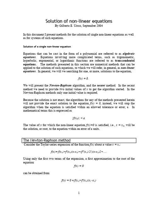
Such approximation is given by, x1 = xo - f(xo)/f'(xo). The Newton-Raphson method consists in obtaining improved values of the approximate root through the recurrent application of equation above. For example, the second and third approximations to that root will be given by and respectively. This iterative procedure can be generalized by writing the following equation, where i represents the iteration number: xi+1 = xi - f(xi)/f'(xi). After each iteration the program should check to see if the convergence condition, namely, |f(x i+1)|<ε, is satisfied. The figure below illustrates the way in which the solution is found by using the NewtonRaphson method. Notice that the equation f(x) = 0 ≈ f(xo)+f'(xo)(x1 -xo) represents a straight line tangent to the curve y = f(x) at x = xo. This line intersects the x-axis (i.e., y = f(x) = 0) at the point x1 as given by x1 = xo - f(xo)/f'(xo). At that point we can construct another straight line tangent to y = f(x) whose intersection with the x-axis is the new approximation to the root of f(x) = 0, namely, x = x2. Proceeding with the iteration we can see that the intersection of consecutive tangent lines with the x-axis approaches the actual root relatively fast. x2 = x1 - f(x1)/f'(x1), x3= x2 - f(x2)/f'(x2),
[matlab二分法程序代码]matlab牛顿迭代法程序代码
![[matlab二分法程序代码]matlab牛顿迭代法程序代码](https://360docs-1393072327.cos.ap-beijing.myqcloud.com/5cd37268a0116c175f0e48ea.webp)
[matlab二分法程序代码]matlab牛顿迭代法程序代码篇一: matlab牛顿迭代法程序代码牛顿迭代法主程序:function?[k,x,wuca,yx]?=?newtonk=1;yx1=fun;yx2=fun1;x1=x0-yx1/yx2;while?abs>tolx0=x1;yx1=fun;yx2=fun1;k=k+1;x1=x1-yx1/yx2;endk;x=x1;wuca=abs/2;yx=fun;end分程序1:function?y1=funy1=sqrt-tan;end分程序2:function????y2=fun1%函数fun的导数y2=x/)-1/) );end结果:[k,x,wuca,yx]?=?newtonk?=8x?=0.9415wuca?=4.5712e-08yx?=-3.1530e-14[k,x,wuca,yx]?=?newtonk?=243x?=NaNwuca?=NaNyx?=NaN篇二: 二十个JA V A程序代码1百分制分数到等级分数package pm;public class SwitchTest {//编写程序,实现从百分制分数到等级分数的转换////>=90 A// 80~89 B// 70~79 C// 60~69 D// public static void main {int s=87;switch{case 10 :System.out.println;break; case 9 :System.out.println;break; case 8 :System.out.println;break;case 7 :System.out.println;break;case 6 :System.out.println;break; default :System.out.println;break; }}}2成法口诀阵形package pm;public class SwitchTest{public static void main{for{for{System.out.print+”\t”); }System.out.println;}}}3华氏和摄氏的转换法package pm;import java.util.Scanner;public class SwitchTest {public static void main {Scanner sc=new Scanner;while {System.out.println;String s = sc.next.trim;if ) {//做摄氏向华摄的转换System.out.println;double db = sc.nextDouble; double db2 = + 32;System.out.println;} else if ) {//做华摄向摄氏的转换System.out.println;double db = sc.nextDouble; double db2 = * 5 / 9;System.out.println + “C”); }else if){ break;}}}}package pm;import java.util.Scanner;public class SwitchTest{public static void main {Scanner sc=new Scanner;boolean flag=true;while {System.out.println; String str = sc.nextLine.trim; if || str.endsWith) {//做摄氏向华摄的转换30cString st = str.substring - 1);double db = Double.parseDouble;//[0,2)//2 double db=Double.valueOf.doubleValue; double db2 = + 32;System.out.println;} else if || str.endsWith) {//做华摄向摄氏的转换String st = str.substring - 1);double db = Double.parseDouble;//[0,2)//2 double db=Double.valueOf.doubleValue; double db2 = * 5 / 9;System.out.println + “C”); }else if){flag=false;}}}}4三个数的最大数package pm;public class SwitchTest {public static void main {int a=1,b=2,c=3,d=0;d=a>b?a:b;d=a>b?:;System.out.println;}}5简单计算器的小程序package one;import java.awt.BorderLayout;import java.awt.GridLayout;import java.awt.event.ActionEvent; import java.awt.event.ActionListener;import javax.swing.JButton;import javax.swing.JFrame;import javax.swing.JPanel;import javax.swing.JTextField;public class Jsq implements ActionListener {private JFrame frame;private JButton[] bus;private JTextField jtx;private JButton bu;private char[] strs;private String d_one = ““;private String operator;public static void main { new Jsq;}/* 利用构造进行实例化*/ public Jsq { frame = new JFrame; jtx = new JTextField; bus = new JButton[16]; strs = “789/456*123-0.+=“.toCharArray; for { bus[i] = new JButton; bus[i].addActionListener; } bu = new JButton; bu.addActionListener; init; } /* GUI 初始化*/ public void init { JPanel jp1 = new JPanel; jp1.add; jp1.add; frame.add; } /* 事件的处理*/ public void actionPerformed { /*获取输入字符*/ String conn = arg0.getActionCommand; /*清除计算器内容*/ if ) { JPanel jp2 = new JPanel; jp2.setLayout); for { jp2.add; } frame.add; frame.pack; frame.setLocation; frame.setVisible; frame.setDefaultCloseOperation;d_one = ““; operator = ““; jtx.setText; return; } /*暂未实现该功能*/if){ return; } /*记录运算符,保存运算数字*/ if ) != -1) { if && ““.equals)) return; d_one = jtx.getText; operator = conn; jtx.setText; return; } /*计算结果*/ if ) { if && ““.equals)) return; double db = 0; if ) { db = Double.parseDouble + Double.parseDouble); jtx.setText; } if ) { db = Double.parseDouble - Double.parseDouble); jtx.setText; } if ) { db = Double.parseDouble * Double.parseDouble); jtx.setText; } if ) { db = Double.parseDouble / Double.parseDouble); jtx.setText; } d_one = db + ““; return; }//界面显示jtx.setText + conn);}}6三角形图案package pm;public class SwitchTest{public static void main{int n=5;for{for{System.out.print;}for{System.out.print;}System.out.println;}}}7输出输入的姓名package pm;import java.util.Scanner;public class SwitchTest{public static void main{String name=null;Scanner sca=new Scanner ; char firstChar; do{System.out.println; name=sca.nextLine; firstChar=name.charAt;}while);System.out.println;}}8一小时倒计时小程序package pm;import javax.swing.JFrame;import javax.swing.JLabel;import javax.swing.JPanel;public class SwitchTest {private JFrame frame;private JLabel jl1;private JLabel jl2;private JLabel jl3;/*主方法*/public static void main {new SwitchTest.getTime;}/*倒计时的主要代码块*/private void getTime{long time=1*3600;long hour =0 ;long minute =0 ;long seconds=0;while{hour=time/3600;minute=/60;seconds=time-hour*3600-minute*60; jl1.setText;jl2.setText;jl3.setText;try {Thread.sleep;} catch {e.printStackTrace;}time--;}}/*构造实现界面的开发GUI */ public SwitchTest{frame = new JFrame;jl1 = new JLabel;jl2 = new JLabel;jl3 = new JLabel;init;}/*组件的装配*/private void init{JPanel jp=new JPanel;jp.add;jp.add;jp.add;frame.add;frame.setVisible;frame.setLocation;frame.setSize;frame.setDefaultCloseOperation; } }9棋盘图案public class Sjx{public static void main{int SIZE=19;for{if{System.out.print;//两个空格}else{System.out.print);//两个空格}}System.out.println;// System.out.print:);for{System.out.print;//一个空格}else{System.out.print+” “);//一个空格}for{System.out.print;//两个空格}System.out.println;}}}10数组输出唐诗package day04;public class ArrayTest {public static void main{char[][] arr=new char[4][7];String s=“朝辞白帝彩云间千里江陵一日还两岸猿声啼不住轻舟已过万重山”; for{for{arr[i][j]=s.charAt;}for{for{System.out.print;}System.out.println;}}}11找出满足条件的最小数package day02;public class Fangk{public static void main{// for{// int q=i/1000;// int b=i/100%10;// int s=i/10%10;// int g=i%10;// if{ // System.out.println; // break; // }// }loop1: for{loop2: for{if{continue loop2;}for{for{if{ System.out.println); break loop1;}}}}}}} Min Number12判断一个数是否是素数package day02;public class Fangk{ public static void main{ int num=14;boolean flag=true;for{flag=false;break;}}if{System.out.println; }else{System.out.println; }}}////////////////////////////////////////////////////////////////////// package day04;import java.util.Scanner;public class A1{public static void main{int n;Scanner sca=new Scanner;System.out.println; n=sca.nextInt;if){System.out.println; }else{System.out.println;}public static boolean isPrimeNumber{ for{if{return false;}}return true;}}13一个数倒序排列package day02;public class Daoxu{public static void main{ int olddata=3758;int newdata=0;while{for{newdata=newdata*10+olddata%10; olddata=olddata/10; }System.out.println;}}}14将一个整数以二进制输出package day04;import java.util.Scanner; public class ArrayTest { public static void main{ int n; Scanner s=new Scanner; System.out.println; n=s.nextInt; for{if)!=0){System.out.print;}else{System.out.print;}if%8==0){System.out.print;}}}}15矩形图案package day02;public class Fangk {public static void main{ int m=5,n=6; for{System.out.print;}System.out.println;for{System.out.print;for{System.out.print; }System.out.print;System.out.println;}for{System.out.print;}}}16猜数字package day02;import java.util.Scanner;public class Csz {public static void main {Scanner s = new Scanner; int num = * 1000); int m=0; for{System.out.println; m=s.nextInt;if{System.out.println;}else if{System.out.println;}else{System.out.println; break;}if{System.out.println; }}if{System.out.println; }}}17.HotelManagerpackage hotel;import java.util.Scanner;public class HotelManager {private static String[][] rooms;// 表示房间public static void main {rooms = new String[10][12];String comm;// 表示用户输入的命令for {for {rooms[i][j] = “EMPTY”;}}//while {System.out.println;Scanner sca = new Scanner; System.gc;comm = sca.next;if ) {search;} else if ) {int roomNo = sca.nextInt;String name = sca.next;in;} else if ) {int roomNo = sca.nextInt;out;} else if ) {System.out.println;break;} else {System.out.println; }}}private static void out {if-1][-1])){ System.out.println;} return; } rooms[-1][-1]=“EMPTY”; System.out.println; private static void in { if-1][-1])){ System.out.println;return;}rooms[-1][-1]=name;System.out.println;}private static void search {for {//打印房间号for {if {System.out.print + “ “); } else {System.out.print + “ “); }}//打印房间状态System.out.println;for {System.out.print;}System.out.println;}}}18.StudentManagerpackage day05.student_manager;import java.util.Scanner;public class StudentManager {static int[][] scores=new int[6][5];static String[] students={“zhangsan”,”lisi”,”wangwu”,”zhaoliu”,”qianqi”,”liuba”}; static String[] courses={“corejava”,”jdbc”,”servlet”,”jsp”,”ejb”};public static void main {for{for{scores[i][j]=*100);}}Scanner s=new Scanner; String comm;while{System.out.println; comm=s.next;if){String para=s.next; avg;}else if){String course=s.next; sort;}else if){String student=s.next; String course=s.next; get;}else if){break;}else{System.out.println; }}}//main end!public static void avg{int sIndex=-1;//int cIndex=-1; for{ if){ sIndex=i; } } if{ for{ if){ cIndex=i; } } } if{ System.out.println; return; } double avg=0.0; if{ for{ avg+=scores[sIndex][i]; } avg/=scores[sIndex].length; System.out.println; }else{ for{ avg+=scores[i][cIndex]; } avg/=scores.length; System.out.println; } } public static void sort{ int[] courseScore=new int[scores.length]; if){//如果求总分的排名//求出每个学生的总分,将成绩存放在courseScore数组中for{ int studentSum=0; for{ studentSum+=scores[i][j]; }courseScore[i]=studentSum; } }else{//如果不是求总分排名int cIndex=-1; for{//找到这门课程的下标if){ cIndex=i; } } if{//如果是一门有效的课程//把scores数组中这一列的值放到courseScore数组中!for{ courseScore[i]=scores[i][cIndex]; } }else{//如果不是一门有效的课程System.out.println; return; } } String[] studentCopy=new String[students.length]; System.arraycopy; for{ for{ if{ int temp=courseScore[i]; courseScore[i]=courseScore[j]; courseScore[j]=temp; String stemp=studentCopy[i];studentCopy[i]=studentCopy[j]; studentCopy[j]=stemp; } } } int order=1; System.out.println; for{ if{ order--; }else{ order=i+1;} System.out.print;System.out.print;System.out.println;order++;}}public static void get{int sIndex=-1;int cIndex=-1;for{if){sIndex=i;}}if{System.out.println;return;}if){//如果求总分int studentSum=0;for{studentSum+=scores[sIndex][j];}System.out.println; return;}for{if){cIndex=i;}}if{System.out.println;return;}System.out.println;}}19.Fivepackage hotel;import java.util.Scanner;/*** 首先在程序第一次运行的时候,构建出棋盘,切以后* 不能再从新构建,知道结束,所以将其放到静态代码块中。
最优化方法三分法+黄金分割法+牛顿法
最优化⽅法三分法+黄⾦分割法+⽜顿法最优化_三等分法+黄⾦分割法+⽜顿法⼀、实验⽬的1. 掌握⼀维优化⽅法的集中算法;2. 编写三分法算法3. 编写黄⾦分割法算法4. 编写⽜顿法算法⼆、系统设计三分法1.编程思路:三分法⽤于求解单峰函数的最值。
对于单峰函数,在区间内⽤两个mid将区间分成三份,这样的查找算法称为三分查找,也就是三分法。
在区间[a,b]内部取n=2个内等分点,区间被分为n+1=3等分,区间长度缩短率=1 3 .各分点的坐标为x k=a+b−an+1⋅k (k=1,2) ,然后计算出x1,x2,⋯;y1,y2,⋯;找出y min=min{y k,k=1,2} ,新区间(a,b)⇐(x m−1,x m+1) .coding中,建⽴left,mid1,mid2,right四个变量⽤于计算,⽤新的结果赋值给旧区间即可。
2.算法描述function [left]=gridpoint(left,right,f)epsilon=1e-5; %给定误差范围while((left+epsilon)<right) %检查left,right区间精度margin=(right-left)/3; %将区间三等分,每⼩段长度=marginm1=left+margin; %left-m1-m2-right,三等分需要两个点m2=m1+margin; %m2=left+margin+marginif(f(m1)<=f(m2))right=m2; %离极值点越近,函数值越⼩(也有可能越⼤,视函数⽽定)。
else %当f(m1)>f(m2),m2离极值点更近。
缩⼩区间范围,逼近极值点left=m1; %所以令left=m1.endend %这是matlab的.m⽂件,不⽤写return.黄⾦分割法1.编程思路三分法进化版,区间长度缩短率≈0.618.在区间[a,b]上取两个内试探点,p i,q i要求满⾜下⾯两个条件:1.[a i,q i]与[p i,b i]的长度相同,即b i−p i=q i−a i;2.区间长度的缩短率相同,即b i+1−a i+1=t(b i−a i)]2.算法描述⾃⼰编写的:function [s,func_s,E]=my_golds(func,left,right,delta)tic%输⼊: func:⽬标函数,left,right:初始区间两个端点% delta:⾃变量的容许误差%输出: s,func_s:近似极⼩点和函数极⼩值% E=[ds,dfunc] ds,dfunc分别为s和dfunc的误差限%0.618法的改进形式:每次缩⼩区间时,同时⽐较两内点和两端点处的函数值。
MATLAB牛顿法源代码
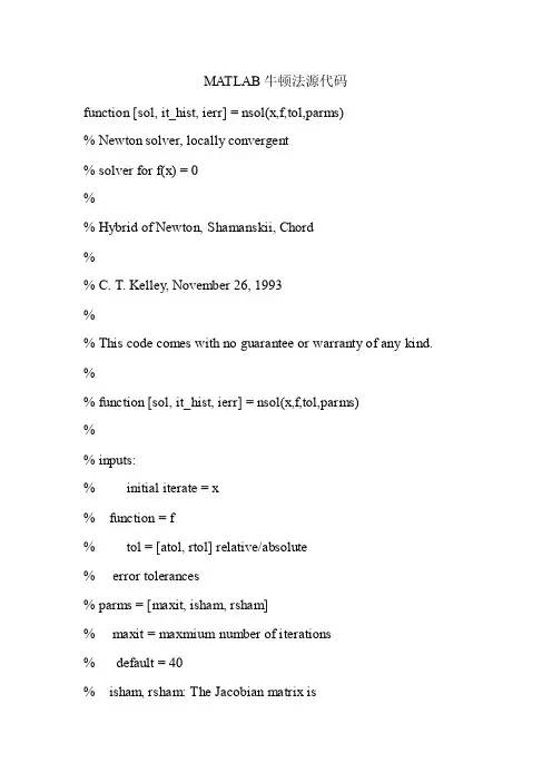
MA TLAB牛顿法源代码function [sol, it_hist, ierr] = nsol(x,f,tol,parms)% Newton solver, locally convergent% solver for f(x) = 0%% Hybrid of Newton, Shamanskii, Chord%% C. T. Kelley, November 26, 1993%% This code comes with no guarantee or warranty of any kind. %% function [sol, it_hist, ierr] = nsol(x,f,tol,parms)%% inputs:% initial iterate = x% function = f% tol = [atol, rtol] relative/absolute% error tolerances% parms = [maxit, isham, rsham]% maxit = maxmium number of iterations% default = 40% isham, rsham: The Jacobian matrix is% computed and factored after isham% updates of x or whenever the ratio% of successive infinity norms of the% nonlinear residual exceeds rsham.% isham = 1, rsham = 0 is Newton's method,% isham = -1, rsham = 1 is the chord method,% isham = m, rsham = 1 is the Shamanskii method % defaults = [40, 1000, .5]%% output:% sol = solution% it_hist = infinity norms of nonlinear residuals% for the iteration% ierr = 0 upon successful termination% ierr = 1 if either after maxit iterations% the termination criterion is not satsified% or the ratio of successive nonlinear residuals % exceeds 1. In this latter case, the iteration% is terminted.%%% internal parameter:% debug = turns on/off iteration statistics display as% the iteration progresses%% Requires: diffjac.m, dirder.m%% Here is an example. The example computes pi as a root of sin(x) % with Newton's method and plots the iteration history.%%% x=3; tol=[1.d-6, 1.d-6]; params=[40, 1, 0];% [result, errs, it_hist] = nsol(x, 'sin', tol, params);% result% semilogy(errs)%%% set the debug parameter, 1 turns display on, otherwise off%debug=0;%% initialize it_hist, ierr, and set the iteration parameters%ierr = 0;maxit=40;isham=1000;rsham=.5;if nargin == 4maxit=parms(1); isham=parms(2); rsham=parms(3); endrtol=tol(2); atol=tol(1);it_hist=[];n = length(x);fnrm=1;itc=0;%% evaluate f at the initial iterate% compute the stop tolerance%f0= feval(f,x);fnrm=norm(f0,inf);it_hist=[it_hist,fnrm];fnrmo=1;itsham=isham;stop_tol=atol+rtol*fnrm;%% main iteration loop%while(fnrm > stop_tol & itc < maxit)%% keep track of the ratio (rat = fnrm/frnmo)% of successive residual norms and% the iteration counter (itc)%rat=fnrm/fnrmo;outstat(itc+1, :) = [itc fnrm rat];fnrmo=fnrm;itc=itc+1;%% evaluate and factor the Jacobian% on the first iteration, every isham iterates, or% if the ratio of successive residual norm is too large %if(itc == 1 | rat > rsham | itsham == 0)itsham=isham;[l, u] = diffjac(x,f,f0);enditsham=itsham-1;%% compute the step%tmp = -l\f0;step = u\tmp;xold=x;x = x + step;f0= feval(f,x);fnrm=norm(f0,inf);it_hist=[it_hist,fnrm];rat=fnrm/fnrmo;if debug==1disp([itc fnrm rat])endoutstat(itc+1, :)=[itc fnrm rat];%% if residual norms increase, terminate, set error flag %if rat >= 1ierr=1;sol=xold;disp('increase in residual')disp(outstat)return;end% end whileendsol=x;if debug==1disp(outstat)end%% on failure, set the error flag%if fnrm > stop_tolierr = 1;enddisp(['iterration number: ',num2str(itc)]);function [l, u] =diffjac(x, f, f0)% compute a forward difference Jacobian f'(x), return lu factors %% uses dirder.m to compute the columns%% C. T. Kelley, November 25, 1993%% This code comes with no guarantee or warranty of any kind. %%% inputs:% x, f = point and function% f0 = f(x), preevaluated%n=length(x);for j=1:nzz=zeros(n,1);zz(j)=1;jac(:,j)=dirder(x,zz,f,f0);end[l, u] = lu(jac);function z = dirder(x,w,f,f0)% Finite difference directional derivative% Approximate f'(x) w%% C. T. Kelley, November 25, 1993%% This code comes with no guarantee or warranty of any kind. %% function z = dirder(x,w,f,f0)%% inputs:% x, w = point and direction% f = function% f0 = f(x), in nonlinear iterations% f(x) has usually been computed% before the call to dirder%% Hardwired difference increment.epsnew=1.d-7;%n=length(x);%% scale the step%if norm(w) == 0z=zeros(n,1);returnendepsnew = epsnew/norm(w);if norm(x) > 0epsnew=epsnew*norm(x);end%% del and f1 could share the same space if storage % is more important than clarity%del=x+epsnew*w;f1=feval(f,del);z = (f1 - f0)/epsnew;。
使用黄金分割法确定步长的牛顿法
//a0为初始步长,b0为初始步长增量;a1,b1为进退法确定的最终区间;
a[0]=a0;
a[1]=a0+b0;
for(i=0;i<2;i++)
for(j=0;j<2;j++)
y[i][j]=x1[j]+a[i]*s1[j];
三、指导教师评语及成绩:
评 语
评语等级
优
良
中
及格
不及格
1.实验报告按时完成,字迹清楚,文字叙述流畅,逻辑性强
2.实验方案设计合理
3.实验过程(实验步骤详细,记录完整,数据合理,分析透彻)
4实验结论正确.
成 绩:
指导教师签名:
批阅日期:
附录1:源 程 序
#include <stdlib.h>
#include <stdio.h>
}while(fabs(c)>eps);
ak2=(m+n)/2;
return ak2;
}
//共轭梯度法
void main()
{
double x[2],s[2],g[4],bita,arph;
//x数组为函数解的转置矩阵;s数组为搜索方向的转置矩阵;g数组为梯度转置矩阵;arph为最优步长;
int k=1;
}
附录2:实验报告填写说明
1.实验项目名称:要求与实验教学大纲一致。
2.实验目的:目的要明确,要抓住重点,符合实验教学大纲要求。
3.实验原理:简要说明本实验项目所涉及的理论知识。
4.实验环境:实验用的软、硬件环境。
matlab实验牛顿法
实验报告实验名称:牛顿法院(系):机电学院专业班级:机械制造及其自动化姓名:学号:2013年5 月13 日实验一:牛顿法实验日期:2013年5 月13 日一、实验目的了解MATLAB的基本运用了解MATLB在优化中的使用二、实验原理牛顿法是梯度法的发展,不仅使用目标函数的一阶导数,而且考虑变化趋势,利用目标函数的二阶偏导,对于一元函数,将其极小点x*附近的一个给定点x0进行泰勒展开,得到二次函数,按照极值条件可得极小值点x1,用其作为x*的下一个近似点,并在x1处进行泰勒展开,得到第二个近似点x2。
直到求的F(x)的极小值点,对于多元函数f(x),同样用上述方法求极小值三、实验内容牛顿法程序:x0=[3;3];%初始点xk=x0;k=0;%迭代变量初始化MLN=100;%最大迭代次数ie=10^(-7);%收敛精度ae=1;%实际收敛精度grad=zeros(2,1);%迭代循环求解while (ae>ie&&k<MLN)syms x1syms x2%调用目标函数,求梯度fun1=fun(x1,x2);fx1=diff(fun1,'x1');fx2=diff(fun1,'x2');fx1=inline(fx1);fx2=inline(fx2);%计算梯度值grad(1)=feval(fx1,xk(1));grad(2)=feval(fx2,xk(2));%计算海赛矩阵及其逆阵G=jacobian(jacobian(fun1),[x1,x2]);b=zeros(2,2);b(1,1)=G(1,1);b(1,2)=G(1,2);b(2,1)=G(2,1);b(2,2)=G(2,2);b=inv(b);xk1=xk-b*grad;ae=norm(xk1-xk);xk=xk1;k=k+1;endx=xk函数程序:function f=fun(x1,x2)f=(x1-1)^4+(x1+2*x2)^2执行结果:x =四、实验小结通过本实验了解了了matlab的基本操作方法,了解牛顿法的原理与基本运用。
最优化方法的Matlab实现(公式完整版)
第九章最优化方法的Matlab实现在生活和工作中,人们对于同一个问题往往会提出多个解决方案,并通过各方面的论证从中提取最佳方案。
最优化方法就是专门研究如何从多个方案中科学合理地提取出最佳方案的科学。
由于优化问题无所不在,目前最优化方法的应用和研究已经深入到了生产和科研的各个领域,如土木工程、机械工程、化学工程、运输调度、生产控制、经济规划、经济管理等,并取得了显著的经济效益和社会效益。
用最优化方法解决最优化问题的技术称为最优化技术,它包含两个方面的内容:1)建立数学模型即用数学语言来描述最优化问题。
模型中的数学关系式反映了最优化问题所要达到的目标和各种约束条件。
2)数学求解数学模型建好以后,选择合理的最优化方法进行求解。
最优化方法的发展很快,现在已经包含有多个分支,如线性规划、整数规划、非线性规划、动态规划、多目标规划等。
9.1 概述利用Matlab的优化工具箱,可以求解线性规划、非线性规划和多目标规划问题。
具体而言,包括线性、非线性最小化,最大最小化,二次规划,半无限问题,线性、非线性方程(组)的求解,线性、非线性的最小二乘问题。
另外,该工具箱还提供了线性、非线性最小化,方程求解,曲线拟合,二次规划等问题中大型课题的求解方法,为优化方法在工程中的实际应用提供了更方便快捷的途径。
优化工具箱中的函数优化工具箱中的函数包括下面几类:1.最小化函数表9-1 最小化函数表2.方程求解函数表9-2 方程求解函数表3.最小二乘(曲线拟合)函数表9-3 最小二乘函数表4.实用函数表9-4 实用函数表5.大型方法的演示函数表9-5 大型方法的演示函数表6.中型方法的演示函数表9-6 中型方法的演示函数表参数设置利用optimset函数,可以创建和编辑参数结构;利用optimget函数,可以获得o ptions优化参数。
● optimget函数功能:获得options优化参数。
语法:val = optimget(options,'param')val = optimget(options,'param',default)描述:val = optimget(options,'param') 返回优化参数options中指定的参数的值。
黄金分割法二次插值法牛顿法matlab程序一维搜索方法比较
牛顿法求解 n 的平方根求解 n 的平方根,其实是求方程 x2−n=0 的解利用上 面的公式可以得到:xi+1=xi−x2i−n2xi=(xi+nxi)/2 编程的时候核心的代码是:x = (x + n/x)/2 三、二次插值法
二次插值法亦是用于一元函数 在确定的初始区间内搜索极小点的一种 方法。它属于曲线拟合方法的范畴。
t=
0.0283
公元前 4 世纪,古希腊数学家欧多克索斯第一个系统研究了这一问题,并建 立起比例理论。
公元前 300 年前后欧几里得撰写《几何原本》时吸收了欧多克索斯的研究成 果,进一步系统论述了黄金分割,成为最早的有关黄金分割的论著。
中世纪后,黄金分割被披上神秘的外衣,意大利数家帕乔利称中末比为神圣 比例,并专门为此著书立说。德国天文学家开普勒称黄金分割为神圣分割。
左边的区间距离 0.0402
黄金分割法所得最小极值点为:-0.993642 黄金分割法所得最小极值为:-0.999960 迭代次数为:9.000000 右边的区间距离 0.0249
左边的区间距离 0.0249
黄金分割法所得最小极值点为:-1.013756 黄金分割法所得最小极值为:-0.999811 迭代次数为:10.000000 右边的区间距边的区间距离 0.7214
左边的区间距离 0.7212
黄金分割法所得最小极值点为:-0.888304 黄金分割法所得最小极值为:-0.987524 迭代次数为:3.000000 右边的区间距离 0.4459
左边的区间距离 0.4459
黄金分割法所得最小极值点为:-1.249028 黄金分割法所得最小极值为:-0.937985 迭代次数为:4.000000 右边的区间距离 0.2755