数理经济学讲义
2010数理经济学讲义(林致远)参考答案
(3)证明
x=y
x= x ( )x x- x =0 给定 x 0, 则有 ( )x 0x 即有 0,从而
(4) 证明
1
数
理
经
济
学
2 0 0 9
秋
季
学
期
( )x ( ( ))x ( )x = x = x x
SFF
因为 F 是闭集,所以 S 是任意包含 S 的闭集的子集。 2.12 证明:集合 S 的内部等于集合 S 减去它的边界,即 int S S \ S 。 证明:任意的 x S 或者是内点或者是边界点。因此,S 的内部是集合 S 中所有的不是 边界点的点 x S
int S S \ b( S )
2.13 证明:集合是有界的,当且仅当它被某些开球所包含。 证 明 : 首 先 , 假 设 S 是 有 界 的 , 令 d d (S ) , 任 选 x S , 对 所 有 的 y S ,
(x, y ) d d 1 。因此 y B(x, d 1) 。S 包含于开球 B(x, d 1) 。
4
数
理
经
济
学
2 0 0 9
秋
季
学
期
一个内点,因此 B int S 。 x 0 是 int S 的一个内点,因此 int S 是开的。 令 G 是 S 的任意一个开的子集, x 是 G 中的一点。G 是 x 的邻域,从而 S G 也是
x 的邻域,因此 x 是 S 的一个内点。从而 int S 包含任意的开的子集 G S ,从而得证 int S
( x1 , x2 ) ( x1 , x2 )
证明: X 是线性空间 证: X1 , X 2 是线性空间 x1 y1 X1 , x2 y2 X 2 ( x1 y1 , x2 y2 ) X1 X 2 类似地,对 ( x1 , x2 ) X1 X 2 , ( x1 , x2 ) X1 X 2 ,因此, X X1 X 2 在加法和 标量乘法下是闭的。 此外,
数理经济学精要
约束为资本的储蓄方程式:
K = I − δ K
§3 变分法
14
例3.1.2 最优资本存量问题
由此问题的 Euler 方程可推导出:
FK
=
⎛ ⎜
r
⎝
+δ
−
p p
⎞ ⎟ ⎠
p
该方程左边表示资本的边际收益,右边表示资本的
实际成本,它等于用投资品价格衡量的利息和折旧
与因资本价格变动带来的收益(购入后资本价格升
§3 变分法
22
可变端点变分问题的Euler方程
【定理 3.2.3】(可变端点变分问题的 Euler 方程和横 截性条件)
设 f ,ψ 为二阶连续可微函数, x∗,t1*为变分法 问题(CVP-4)的最优解,则 Euler 方程(3.1.2)成立,且 满足下述边界条件
⎡⎣ f (t, x∗, x∗ ) + (ψ − x∗ ) fx (t, x∗, x∗ )⎤⎦t=t1* = 0 (3.1.7)
(3.1.4)
L(t, x(t), x(t)) = f (t, x(t), x(t)) + μT g(t, x(t), x(t))。
§3 变分法
17
例3.2.1:等周问题
如下图,考虑连接两点 A、B 的长度为一定的, 与线段 AB 围成的面积最大的曲线。
y
A
B
x0 图 3.2.1 等周问题 x1 x
厦门大学经济系 邵宜航
数理经济学精要
——经济学中的最优化数学分析
变分法原理与应用 (讲义要点)
第三章 变分法
§3.1 最简变分问题 §3.2 条件变分和可 动边界变分
3.1.1. 最简泛函的第一 变分与第二变分
数理经济学 课件

ccer05研究生数理经济学讲义2
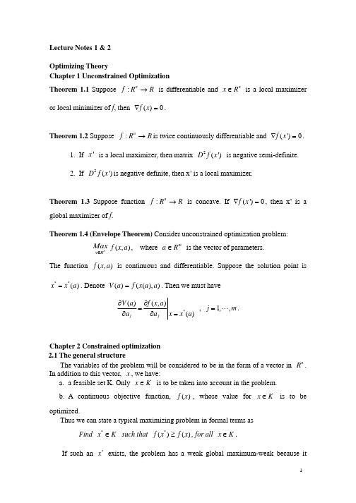
Lecture Notes 1 & 2Optimizing TheoryChapter 1 Unconstrained OptimizationTheorem 1.1 Suppose :n f R R → is differentiable and n x R ∈ is a local maximizer or local minimizer of f , then ()0f x ∇=.Theorem 1.2 Suppose :n f R R →is twice continuously differentiable and (')0f x ∇=.1. If 'x is a local maximizer, then matrix 2(')D f x is negative semi-definite.2. If 2(')D f x is negative definite, then x’ is a local maximizer.Theorem 1.3 Suppose function :n f R R → is concave. If (')0f x ∇=, then x’ is a global maximizer of f .Theorem 1.4 (Envelope Theorem) Consider unconstrained optimization problem:n x RMax ∈(,)f x a , where m a R ∈ is the vector of parameters. The function (,)f x a is continuous and differentiable. Suppose the solution point is **()x x a =. Denote ()((),)V a f x a a =. Then we must have*()(,)()j j V a f x a x x a a a ∂∂==∂∂ , 1,,j m =".Chapter 2 Constrained optimization2.1 The general structureThe variables of the problem will be considered to be in the form of a vector in n R . In addition to this vector, x , we have:a. a feasible set K. Only x K ∈ is to be taken into account in the problem.b. A continuous objective function, ()f x , whose value for x K ∈ is to be optimized.Thus we can state a typical maximizing problem in formal terms asFind *x K ∈ such that *()()f x f x ≥, for all x K ∈.If such an *x exists, the problem has a weak global maximum-weak because itsatisfies the weak inequality, global because the inequality is satisfied for all x K ∈. A global optimum should not be confused with an unconstrained optimum. The latter implies that n K R =. We would have a strong maximum if we could find *x such that *()()f x f x >, for all x K ∈.A weak optimum is equivalent to a non-unique optimum point since any x satisfying *()()f x f x = is also an optimum point. A strong global optimum implies a unique optimum.If we reverse the inequalities we obtain a minimum, weak or strong as the case may be. A minimum for ()f x implies a maximum for [-()f x ]. The value *x is often called simply the solution of the optimum problem. To avoid confusion with other claimants for the same name in many economic models, we shall usually call it the optimal solution or optimum point.Most calculus techniques cannot solve the problem as set out above, but can only solve a problem of the following kind:Find *x K ∈ such that *()()f x f x ≥, for all ()x N K ∈∩,where N is a neighborhood of *x .Such a point is a weak local maximum. We can have a weak or strong local maximum, and weak, or strong local minimum.It is obvious that a global optimum must also be a local optimum. Nevertheless, a local optimum is not necessarily global. Our interest is primarily in the global optimum. Thus, we are interested in conditions on the structure of the problem that will guarantee that a local optimum is also global. If such conditions are not satisfied, we need to adopt ad hoc procedures to locate the global optimum.2.2 Constraints and the Feasible SetThe feasible set, over which the variables are permitted to range, may be defined in any suitable way. In the case of discrete variables, the feasible set may even be described by enumeration. Typically, however, the feasible set will be defined by equalities or inequalities involving relationships between the variables.The boundaries of the feasible set are crucial in optimizing problems. In all our discussions of optimizing, it will be assumed that the constraints are such that as to give a closed feasible set. Otherwise the problem is usually without a solution. This is normally guaranteed by ensuring that there are no strict inequalities in any of the constrains and that the constraints are continuous.When there are several constraints, given a feasible point x ’, we say that a particular constraint is effective at x ’ if x ’ gives an equality in the constraint, ineffective at x ’ if it gives an inequality. Note that a constraint may be “effective” in a common sense meaning without being effective this technical sense.2.3 The General Optimizing ProblemThe Standard format:Max ()f x , n x R ∈, s.t. (1) ()0,i g x ≤ 1,...,i m =; (2) 0k x ≥, {1,...,}k S n ∈⊂. Function ()f x is the objective function; x is the variable vector of the problem. The constraints (1) are the functional constraints, the constraints (2) are the direct constraints. The functions are assumed to be continuous.It is convenient to have all the inequalities in the same direction in the same direction in a standard form. Obviously 00f f ≥⇔−≤.The functional constraints can always be put in inequality form by noting that 00&0f f f =⇔≤−≤. For a very important case of the general problem, all the constraints are equalities and it is then easier to drop the inequality form.The direct constraints will always be written in the nonnegative form. The inequalities in both the functional and direct constraints are assumed always to be weak inequalities to ensure that the feasible set is closed.An optimum problem need not have a solution in general. However, we do have a guarantee that the problem is worth pursuing in a large class of cases:Theorem 2.1 (Weierstrass): A continuous function defined over a nonempty closed bounded set attains a maximum and a minimum at least once over the set.Since we usually take the objective function to be continuous and the feasible set to be closed, the boundedness of the feasible set is the only condition that is not ensured. Nevertheless, Weierstrass theorem gives sufficient but not necessary conditions to the existence of a solution of an optimum problem.2.4 The General Solution PrincipleAn optimal point must be in the feasible set but may be either an interior point or a boundary point. If it is an interior point, it has a neighborhood of feasible points and must be an optimum relative to those neighborhood points. Such a point must satisfy the ordinary calculus conditions for an unconstrained optimum. A boundary point has a neighborhood that includes infeasible points as well as feasible ones, and it is not possible to say that such a point must be optimal relative to its neighborhood. A boundary optimal point need not be critical point of f .f x are Proposition 2.2 The solution to the general optimum problem, where ()f x for x over some closed feasible set K will, if it exists, be some differentiable, Max()f x, or (b) a boundary point of K (or both). point x’ which is: (a) a critical point of ()In principle, an optimum problem can be solved by finding the critical points of ()f x along the boundary, finally choosing the f x, then computing the values of ()f x is not differentiablef x. If ()point giving the maximum or minimum of ()everywhere, the points at which it is not differentiable will need to be examined in addition to the critical and boundary points.2.5 Conditions for a Global optimumSince we are usually interested in a global optimum and since many techniques discover only local optima, conditions which guarantee that a local optimum is also a global optimum are of great value. The particular conditions set out below are of special importance because they are satisfied by most typical optimum problems in economicsf x Proposition 2.3 For problem concerned with optimizing a continuous function ()f x over a closed feasible set K, every local optimum is also a global optimum if: (a) () is a concave function for a maximum, or convex function for a minimum; and (b) K is a convex set.f x is strictly concave over a convex feasible set the global Proposition 2.4 If ()optimum is unique.Chapter 3 Classical Calculus Methods3.1 IntroductionClassical calculus methods deal with problem with the following properties:a). The objective and indirect constraint functions possess suitable continuityproperties. Usually they will be taken to be of class 2C.b). The functional constraints are equalities.c). There are no direct (non-negativity) constraints on the variablesThe standard form of the problem will be written asMax ()f x , s.t. ()0,i g x = i =1,…,m (m<n )Since the constraints are all effective at all times, the feasible set K contains only boundary points, so interior optima are ruled out. Unless the constraints are all linear, K will not necessarily be a convex set.If the appropriate Jacobean is nonsingular, we can express n-m of the variables in terms of the remaining m (from the implicit function theorem). Hence, we can reduce the problem to one of the unconstrained optimization of a function of only n-m variables. However, explicit solution of the constraint equations is possible only in a few cases, if these are nonlinear.3.2 The Lagrangean FunctionLet us examine the properties of a function 1(,)()()mi i i L x f x g x λλ==−∑, wherethe λ’s are arbitrary variables. The function (,)L x λ is called the Lagrangean function, and the λ’s are Lagrange multipliers.If we take the derivatives of (,)L x λ with respect to the λ’s, we have (,)/()0i i L x g x λλ∂∂=−= for x K ∈. Hence if (,)L x λhas a critical point at ','x λ, then 'x K ∈. Also for x K ∈, (,)L x λ=()f x . It can be shown that if x ’ maximizes f(x) over K, there is some 'λ such that (','x λ) is a critical point of (',')L x λ. The results hold for a minimum as well as a maximum.To use the Lagrange technique, we set up the Lagrangean and then find its critical point(s). The partial derivatives of (,)L x λ with respect to λ’s are simply the constraint functions and equating them to zero merely ensures that x K ∈. It is the partial derivatives with respect to the x ’s that play the major solution role. If these are equated to zero, we obtain n equations of:1mi j i j i f g λ==∑, (1,...,)j n = We can write it as f G λ∇=, where []ij G g = and []i λλ=3.3 Interpretation of the Lagrange MultipliersConsider a standard classical optimizing problem, solved by the Lagrangean technique to give solution values ','x λ. Let the i th constraint be of the form ()i i g x b =. Initially suppose 0i b =. We wish to examine the result of a small relaxation of thisconstraint.Denote the optimal value of the objective function by V’. Now a small relaxation in the i th constraint will permit small changes in the optimal values of the variables, but we assume the optimum conditions remain satisfied so that the new position reached as a result of this relaxation is also optimal. The effect on the optimal value of the objective function will be given by '(')j j i j i x V f x b x b ∂∂∂=∂∂∂∑ (1)From the constraints we have 0(')1k j j j i x k i g x k i x b ∂≠⎧∂=⎨=∂∂⎩∑ (2)If we multiple the k th equation in (2) by 'k λ, and sum over k , we obtain''(')k j ki k j j i x g x x b λλ∂∂=∂∂∑∑ With (1), we have''(')[i j i j V f x b x λ∂∂=+−∂∂∑(')]k j k kj i x g x x b λ∂∂∂∂∑='i λ Thus 'k λ corresponds to the marginal rate of change of the optimal value of the objective function with respect to a small relaxation of the i th constraint, other constraints being unchanged. In typical economic applications, the constraints might be resource limitations and the objective function is index of some social welfare. The optimal Lagrange multipliers would then correspond to the marginal social valuation of the resources.Proposition 3.1 (Envelope theorem) Let (,)f x r and (,)i g x r for i =1,…,m be continuously differentiable functions of the n+k variables. Consider the following optimizing problem:x Max (,)f x r , s.t. (,)0,i g x r = i =1,…,m (n x R ∈, m<n, k r R ∈)Denote the solution of the problem as *()x r , and **()((),)f r f x r r =. Suppose *()x r and the associated Lagrange multipliers 1,...,m λλ are continuously differentiablefunctions of r and the rank of the *[()]ij g x is m . Then**()(,)h hf r L x r r r ∂∂=∂∂ for h=1,…,k ,where 1(,)(,)(,)mi i i L x r f x r g x r λ==−∑.Example : Consider a utility maximization problem: xMax ()u x , s.t. p x w ⋅= Denote the solution of the problem by *(,)x p w , and *(,)((,))v p w u x p w ≡. Function (,)v p w is known as the indirect utility function . By the envelope theorem, we have**(,)(,)(,)i i v p w p w x p w p λ∂=−⋅∂, and *(,)(,)v p w p w wλ∂=∂. Hence we have*/(,)/i v p x p w v w∂∂=−∂∂. This result is known as Roy’s Identity .Chapter 4 Advanced Optimizing Theory4.1 IntroductionThe classical method, assumes both equality in the functional constraints and the absence of direct constraints on the variables. Although this method is widely employed in economic analysis, the fact is that most economic problems have implicit, if not explicit, properties that do not entirely fit the classical case. Nonnegative constraints on at least some variables are usually implicit, and the functional constraints may be more accurately described by inequalities than equalities. Consider the following problem of a consumer.Max 12(1)(1)u x x =++, s.t. 1241x x +=If we solve the problem, using traditional methods, we obtain the optimal values for x as *(1/4,2)x =−, with the optimal level of utility, *9/4u =. Direct calculation shows, however, that (0,1) is optimal, given the nonnegative condition.4.2 Nonnegative VariablesThe most straightforward extension of the classical calculus method is to the case in which some or all of the variables are subject to direct constraints. Consider thisMax f(x) s.t. ()0i g x =, (1,...,i m =), 0x ≥. (3)We can define the function (,)L x λ in the usual way. Three situations are possible. a). (,)L x λ has a regular local maximum at a critical point **(,)x λ, with *0x >, andthe problem satisfies the strong global optimum conditions.b). (,)L x λ has a regular local maximum at a critical point, with *0x >, but the strong global optimal conditions are not satisfied.c). (,)L x λ does not have a critical point with *0x >, which is also a local maximum.The first case is presumed to occur in traditional economic analysis. In the third case, the global optimum must be at a point at which some non-negativity constraint is operative. In the second case it might be at such a point, and will usually need to check.Still with problem (3), consider the properties of (,)L x λ and ()f x at a point x K ∈ at which 0k x = for at least one k . Since the functional constraints 0i g = are still equalities, the maxima of (,)L x λ and ()f x , x K ∈ still occur at the same point *x . Also we still have /0i L λ∂∂=, but what about the first order conditions /0j L x ∂∂=? In general, they might not all be satisfied.Define (){{1,...,}|0}i S x i n x =∈=. If ()j S x ∉, small variations in j x are possible in both positive and negative directions, so that x cannot be optimal unless /0j L x ∂∂=. If ()j S x ∈, small variations in j x are possible in the positive directiononly, so that x cannot be optimal if /0j L x ∂∂>. But small variations are not possible inthe negative direction, so we cannot rule out /0j L x ∂∂< asnon-optimal.Proposition 4.1 The optimal point *x of the problem (1) satisfies the following conditions: 1) ***1(,)0m i j i j i j L x f g x λλ=∂=−≤∂∑, and ****(,)0j j L x x x λ∂⋅=∂, 1,...,j n =. 2) ***(,)()0i iL x g x λλ∂=−=∂Example Let us return to the earlier example, which shall be stated asMax 12(1)(1)u x x =++, s.t. 1241x x +=; 12,0x x ≥The first order derivatives are 12/14L x x λ∂∂=+−, 21/1L x x λ∂∂=+−, and12/41L x x λ∂∂=+−. We already know that there is no critical point of L with 12,0x x >. Now we try putting 1x , then 2x to zero, given the budget constraints. At (0,1), we have21/110L x x λλ∂∂=+−=−=, whichgives 1λ=. 12/14L x x λ∂∂=+−= -2. U =2At (1/4,0), we have12/14140L x x λλ∂∂=+−=−=, which gives 1/4λ=. 21/11L x x λ∂∂=+−=>0, So (1/4, 0) is not an optimal point.There is no universal rule for determining which variables, when put to zero, are likely to lead to an optimal solution. In principle, we may have to try putting one variable at a time to zero, then two at a time, three at a time, and so on, and then compare the results of all cases that satisfy the optimal conditions.In economic analysis, however, we are usually interested in what happens to the optimal conditions when we do have a solution on the nonnegative boundary, and to this we have the answer. Furthermore, boundary problems of this kind in economic frequently occur as the result of a movement to the boundary from an interior point as some parameter is changed, so that the zero variables are specified for us.4.3 Inequality ConstraintsWe now consider the general optimum problem, with the two restrictions of the classical calculus method removed:Max ()f x s.t. ()0i g x ≤, (1,...,i m =), 0x ≥. (4)The problem can be converted into the case discussed in the preceding section by adding slack variables i z to give the i th constraint as ()0i i g x z +=, 0i z ≥.There are now n+m variables in the problem, an n -vector of x variables and an m -vector of z variables, with non-negativity constraints on all. We form the Lagrangean1(,,)()(())m i i i i L x z f x g x z λλ==−+∑=11()()m mii i i i i f x g x z λλ==−−∑∑ The optimal conditions with respect to j x are as before. The optimal conditionswith respect to i z are ***(,)0i i L x z λλ∂=−≤∂, and 0i i z λ=. These conditions impose no direct constraints on x , Their content is entirely represented by the equivalent statement()0i g x ≤, (1,...,i m =), 0λ≥, and 1()0miii g x λ==∑. Thus if we form the Lagrangean, ignoring the inequalities in the functional constraints, as 1(,)()()mi i i L x f x g x λλ==−∑, adding the non-negativity constraint 0λ≥,all points which are optimal for z in (,,)L x z λ satisfy (,,)L x z λ(,)L x λ=. Consider (,)()i iL x g x λλ∂=−∂. From the constraints we have ()0i g x ≤, and from the optimal conditions with respect to z in (,,)L x z λ, we have 0λ≥ and ()0i i g x λ⋅=. These together imply (,)0iL x λλ∂≥∂ and (,)0i i L x λλλ∂⋅=∂. The above conditions can be recognized as the conditions for a minimum of (,)L x λ with respect to λ, given the non-negativity constraint 0λ≥.How does it come about that, although we are seeking a maximum for ()f x subject to the constraints, and although we were able to treat (,)L x λ as having a maximum with respect to x in the strict classical case, we now seek a minimum with respect to λ of the expression that is analogous to the strict classical Lagrangean?First, we note that, in the strict classical case, if (,)L x λ is neutral with respect to changes in λ over the feasible set, we would have regarded (,)L x λ as having a minimum with respect to λ just as well as having a maximum.Second, we note that at any optimal point of (,)L x λ, whatever a maximum or a minimum with respect to λ, we have (,)L x λ()f x =. Whether a maximum or a minimum is involved, with respect to λ, is related to the constraints but not to the objective function.Third, consider an effect of a small variation in λ from its optimal value *λ. If*λ>0, then **(,)L x λ isunchanged. If *λ=0, we may have *()0i g x <. Because of the nonnegative constraint on λ, the only permissible variation is to some small positive value. In this case, the term ()i i g x λ− in the expression of **(,)L x λ will take on apositive value and we will have *(,')L x λ>**(,)L x λ. Thus, the optimal point gives a minimum of (,)L x λ. The minimum property will only be apparent when at least one constraint is ineffective.Proposition 4.2 (Kuhn-Tucker Conditions) The optimal point *x of the problem (4) satisfies the following conditions: (1) ***1(,)0m i j i j i j L x f g x λλ=∂=−≤∂∑; ****(,)0j jL x x x λ∂⋅=∂, 1,...,j n =. (2) *()0i g x ≤, and *0λ≥; **()0i i g x λ⋅=.If the problem is one of minimizing, the direction of the inequalities in (1) is reversed. If we are not trying to discover whether a certain point is optimal or not, but are merely interested in the properties of a point already known to be optimal, conditions (2) state that we can ignore ineffective constraints at the optimum.We have noted that (,)L x λ, a function of two sets of variables, has a maximum with respect to x and minimum with respect to λ at the optimum. A point which gives a maximum of a function with respect to some variables, and minimum with respect to others, is called a saddle point, a term descriptive of the shape of the function in three dimensions.4.5 Existence of Optimal SolutionsConsider the Lagrangean written in the form 1(,)()()mi i i L x f x g x λλ==−∑, with theconstraints 0,0,x λ≥≥()0i g x ≤. We see that (,)L x λ is a concave function of x if ()f x is concave and each ()i g x is convex. Considering the sets over which ,x λ are confined, since λ is defined on a convex set and the set {|()0}i x g x ≤ is convex when ()i g x is convex, the feasible set is the intersection of convex sets and is convex.We still need the sets to be compact. The nature of the constraint inequalities ensures that they are closed, so it remains to consider boundedness. Since we seek a minimum for λ, and it is bounded below by the non-negativity constraint, we can impose an arbitrary upper bound so large it does not affect the optimal solution. The feasible set for x presents the difficulties. We cannot avoid adding the special assumption that thefeasible set is bounded.Thus if ()f x is concave, every ()i g x is convex and the feasible sets is bounded, the Lagrangean satisfies the conditions of Theorem 4.4, so that is possesses a saddle point and the general optimizing problem possesses a solution. Furthermore, the conditions for a global optimum are satisfied by the same convexity-concavity conditions. Thus we haveTheorem 4.5 The general maximum problem ()Maxf x s.t. ()0i g x ≤, (1,...,i m =), 0x ≥. Always possesses a solution if:a). ()f x is concave and every ()i g x is convex;b). the feasible set {|()0,1,...,;0}i K x g x i n x =≤=≥ is bounded and nonempty.Under these conditions the Lagrangean 1(,)()()mi i i L x f x g x λλ==−∑ possesses asaddle point **,x λ, where *x is optimal in the maximum problem and *0λ≥. Furthermore, the values **,x λ satisfy the Kuhn-Tucker conditions, which are then sufficient for a global optimum. If ()f x is strictly concave, the point *x is unique.Homework:1. If 221122()2f x x bx x x =++, what values of b give: a). a local maximum of f(x), s.t. 121x x += ?b). a local minimum for f(x), s.t. 121x x += ?2. The welfare function for a two-good, two-person economy is 112a a W u u −=. Theindividual utility functions are 111121b b u x x −=, 121222c c u x x −=, where ij x is the amount of thei th good consumed by the j th individual.If the total amounts of the two goods are fixed, what is the optimum allocation between the two individuals? (Assume ,,]0,1[a b c ∈)3. Discuss the nature of the optimum solution for different values of a in the problem:Max 221210(2)(2)x x −−−− s.t. 22121x x +≤, 12x x a +≤, 120,0x x ≥≥.。
数理经济学讲义
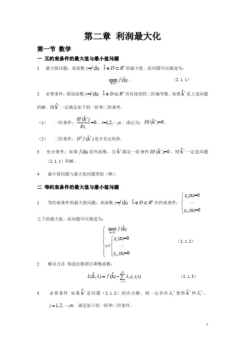
第二章 利润最大化第一节 数学一 无约束条件的最大值与最小值问题1 最大值问题:求函数=(x)y f nx D R ∈⊂的最大值。
此问题可以描述为:x max (x)Df ∈。
(2.1.1)2 必要条件:假设函数=(x)y f n x D R ∈⊂具有连续的二阶偏导数。
如果x *是上述问题的解,则x *一定满足如下的一阶和二阶条件。
(1) 一阶条件:(x )=0if x *∂∂,=1,2,,i n ⋅⋅⋅。
或记为:(x )=0Df *。
(2) 二阶条件:2(x )D f *是半负定矩阵。
3 充分条件:如果(x)f 是凹函数,且x *满足一阶条件(x )=0Df *,则x *一定是问题(2.1.1)的解。
4 最小值问题与最大值问题类似(略)。
二 等约束条件的最大值与最小值问题1 等约束条件的最大值问题:求函数=(x)y f nx D R ∈⊂在约束条件:1(x)=0(x)=0mg g ⎧⎪⋅⋅⋅⎨⎪⎩之下的最大值。
此问题可以描述为:x 1.max (x)(x)=0(x)=0Dmf g s t g ∈⋅⎧⎪⎪⎧⎨⎪⎨⎪⎪⋅⎩⋅⎪⎩ (2.1.2)2 解决方法 构造拉格朗日乘数函数: 1(x,)(x)()mjjj L f g x λλ==-∑ (2.1.3)3 必要条件 如果x *是问题(2.1.2)的内点解,则一定存在j λ*使得x *和j λ*,1,2,,j m =⋅⋅⋅,满足如下的一阶和二阶条件。
(1) 一阶条件:1(x ,)()()0m j j j j ii i L g x f x x x x λλ****=∂∂∂=-=∂∂∂∑, 1,2,,i n =⋅⋅⋅(x ,)()0j j jL g x λλ**∂=-=∂, 1,2,,j m =⋅⋅⋅一阶条件共n m +个。
(2) 二阶条件:二阶条件比较复杂。
这里只给出一个约束条件下的二阶条件。
当只有一个约束条件()0g x =时,二阶条件为:对任何满足线性约束的()Dg x h 的向量h ,都有:2()0h D g x h τ≤ 4 最小值问题与最大值问题类似(略)。
《数理经济学》课件

数学符号在数理经济学中具有特定的意义,它们代表了经济变量、参数和函数等。理解这些符号的意义 是理解数理经济学理论的关键。
数学模型与方程
01
模型构建
数理经济学家使用数学模型来描述经济系统。这些模型通常由一组方程
式构成,用来表示不同经济变量之间的关系。
02
方程类型
在数理经济学中,常见的方程类型包括线性方程、非线性方程、微分方
数理经济学的发展历程
总结词
数理经济学的发展历程可以追溯到19世纪,其发展经 历了多个阶段,包括古典数理经济学、新古典数理经 济学和现代数理经济学等。
详细描述
数理经济学的发展历程可以追溯到19世纪,当时一些 经济学家开始尝试运用数学方法来描述和预测经济现 象。古典数理经济学阶段主要关注生产、分配和交换 等经济活动的均衡问题。新古典数理经济学阶段则强 调个体行为和市场均衡的研究,并引入了边际分析和 效用函数等概念。现代数理经济学则更加注重数学模 型的复杂性和精确性,并广泛应用于宏观和微观经济 学等领域。
在数理经济学中,证明方法多种多样 ,包括直接证明、反证法、归纳法和 演绎法等。这些方法用于证明经济定 理和推导经济关系,确保经济理论的 严谨性和准确性。
在数理经济学中,必须遵循一定的推 理原则,如公理化原则、一致性原则 和完备性原则等。这些原则确保了经 济理论的逻辑严密性和科学性。
03
数理经济学的应用
宏观经济学中的应用
经济增长与经济发展
数理经济学在研究经济增长、经济发展等方面发挥了重要作用,通 过建立数学模型来解释国家或地区的经济增长和发展趋势。
财政政策与货币政策
利用数理经济学方法分析财政政策和货币政策的效果,为政府制定 经济政策提供科学依据。
数理经济学-数理经济学本083jok-PPT精品文档

A
1
21
练习4:利润率=1时,求供给函数及要素需求函数。
L bp Y w
p r w 要素 需求函数 L/Y
1 1
1 A
22
练习4:利润率=1时,求供给函数及要素需求函数。
1 1 1 1 1 1 1 p a r b w A
练习:请写出生产函数表达式
27
N1原材料面粉消耗 N2原材料调料消耗 K固定资本 生 产 函 数 Q产出数量
生 产 L 函 数
V增加值
28
N1原材料面粉消耗 N2原材料调料消耗 K固定资本 生 产 函 数 Q产出数量
生 产 L 函 数
V增加值
N 1 N 2 Q min , ,V 1 b 2 b
数理经济学丶课间休息
1
第3 讲
第2章:生产函数与供给函数 及要素需求函数
2
了解生产函数与供给 函数及要素需求函 数在实际中的应用
3
r
利润最大决策
K
生 产 函 数 Y
w
Max Y s.t rK+wL=C
L
C
4
练习1:
写出生产函数的数学表 达式并画出等产量线。
5
练习1:写出生产函数的数学表达式
Max S.t
Y Y (K, L) r K w L C
Y 1 Y 1 K r L w
13
练习3:边际利润率=利润率?
Max Y Y(K, L) S.t r K wL C Y p Y p pY ? K r L w C
1 1
A A
1
1 1
数理经济学讲义

1.0.3 经济分析中使用数理方法的好处ice between literary logic and mathematical logic, again, is a matter of little import, but mathematics has the advantage of forcing analysts to make their assumptions explicit at every stage of reasoning. This is because mathematical theorems are usually stated in the “if-then” form, so that in order to tap the “then” (result) part of the theorem for their use, they must first make sure that the “if” (condition) part does conform to the explicit assumptions adopted.
• P.Samuelson提出了新古典综合体系。 • 20世纪70年代以来,经济动态分析逐渐兴起
和快速发展。
数理经济学讲义
1.0.3 经济分析中使用数理方法的好处
• 数理经济学与非数理经济学 • Since mathematical economics is merely an approach to economic
数理经济学讲义
1.0.2 数理经济学的历史发展
• 数理经济学的先驱是法国学者A.A.Cournot,他于 1838年发表了《以数学原理研究财富的理论》,提 出了需求函数理论,把人们熟视无睹的商品需求量 与价格之间的关系写成了函数形式。
- 1、下载文档前请自行甄别文档内容的完整性,平台不提供额外的编辑、内容补充、找答案等附加服务。
- 2、"仅部分预览"的文档,不可在线预览部分如存在完整性等问题,可反馈申请退款(可完整预览的文档不适用该条件!)。
- 3、如文档侵犯您的权益,请联系客服反馈,我们会尽快为您处理(人工客服工作时间:9:00-18:30)。
第一章生产技术第一节微观经济学简介一什么是微观经济学?微观经济学以单个经济单位(单个生产者,单个消费者,单个市场的经济活动)作为研究对象,分析个体生产者如何将有限的资源分配在各种商品的生产上以取得最大的利润;单个消费者如何将有限的收入分配在各种商品的消费上以获得最大的满足。
同时微观经济学还分析单个生产者的产量、成本、投入要素的数量、利润等如何确定;生产要素的供给者的收入如何确定;单个消费品的效用、供给量、需求量和价格等如何确定。
简单地说,微观经济学是研究经济社会中单个经单位的经济行为,以及相应的经济变量的单项数值如何决定的经济学说。
二微观经济学的发展和形成简介微观经济学的发展迄今为止大体上经历了四个阶段。
第一个阶段十七世纪中期到十九世纪中期是最早期微观经济学阶段,或者说是微观经济学的萌芽阶段。
代表人物主要有斯密和李嘉图。
第二个阶段十九世纪晚期到二十世纪初叶是新古典经济学阶段,也就是微观经济学的奠基阶段。
在这个期间,杰文斯在英国,门格尔在奥地利,瓦格拉斯在瑞士顺次建立了英国学派,奥地利学派和洛桑学派。
这三个学派的学说并不完全一致,但它们具有一个重要的共同点,那就是放弃了斯密和李嘉图的劳动价值论,并提出了边际效用价值论。
在此之后,英国经济学家马歇尔以三个学派的边际效用价值论和当时其它的一些论述(如供求论,节欲论,生产费用论)为基础构建了微观经济学的理论框架,再加上庇古,克拉克和威克斯迪等人提出的新观点形成了以马歇尔和瓦尔拉斯为代表的新古典经济学。
第三个阶段二十世纪三十年代到六十年代是微观经济学的完成阶段。
在这个阶段,凯恩斯的传人萨缪尔森建立了新古典综合学派的理论体系。
他把以希克斯(代表作《价格与资本》)为代表的经济学家对马歇尔的理论框架进行的修改和补充成为研究个量的微观经济学,把经过修改和补充之后的凯恩斯理论称之为宏观经济学。
至此完成了微观经济学的理论体系。
第四个阶段二十世纪六十年代至今是微观经济学进一步发展,补充和演变阶段。
四高级微观经济学的特点初级微观经济学主要介绍一个或两个生产要素和一种产品的情况,数学工具也用的较少。
高级微观经济学介绍的则是多种生产要素和多种产品的情况,运用的数学工具也很多。
第二节 数学一 导数和偏导数1 导数:定义及其意义。
2 偏导数和海塞矩阵二 函数的性质1 单调性2 齐次函数和位似函数(a ) 齐次函数的定义:设12()(,,)n y f x f x x x ==⋅⋅⋅是一个n 元函数,其中12(,,)n n x x x x D R =⋅⋅⋅∈⊂,如果0t ∀>,有()()k f tx t f x =,则称()f x 是一个k 次齐次函数。
注: 当1k ≥时,k 次齐次函数的一阶偏导数是1k -次齐次函数。
欧拉定理:若()f x 是一个k 次齐次函数,则1()()ni ii f x xkf x ==∑(b )位似函数由一个正的单调函数()g 和一次齐次函数()f x 构成的复合函数(())g f x 称为一个位似函数。
三 集合的凸性,函数的凸性及拟凸性1 集合的凸性(定义)2 凸函数与凹函数四 上轮廓集(uper contour set )和拟凹函数(quasiconcave function )1 上轮廓集 设()f x ,nx D R ∈⊂是一个函数,对给定的实数a 称集合 {,()}A x x D f x a =∈≥ 为函数()f x 的一个上轮廓集。
集合{,()}B x x D f x a =∈= 为函数()f x 的一个水平集2 拟凹函数与拟凸函数如果a R ∀∈,()f x 的上轮廓集都是凸集,则称()f x 是一个拟凹函数;如果()f x -是一个拟凹函数,则称()f x 是一个拟凸函数。
3 结论:函数()f x 是拟凹函数的充分必要条件是:12,x x D ∀∈及[0,1]t ∈,有 1212((1))min{(),()}f tx t x f x f x +-≥第三节 生产函数一 生产可能集如果一个厂商投入n 种生产要素12(,,)n x x x x =⋅⋅⋅,生产出k 种产品12(,,)m y y y y =⋅⋅⋅,这里0,0;1,2,,;1,2,,i j x y i n j m ≥≥=⋅⋅⋅=⋅⋅⋅。
则称1212(,)(,,,,,,,)m n Z y x y y y x x x =-=⋅⋅⋅--⋅⋅⋅-为净产出向量,它描述了该厂商的一个可行的生产方案。
所以可行的生产方案构成的集合称为生产可能集。
在这里我们主要讨论n 种生产要素,一种产品的情况。
此时生产可能集是由所有可行的生产方案12(,)(,,,,)n y x y x x x -=--⋅⋅⋅- 构成的集合。
二 生产函数1 定义:假设厂商在生产时满足两个条件,第一,生产是有效率的;第二,满足无成本处置条件,即可以无成本地不要的资源。
在这样的条件下,对厂商的每组n 种生产要素的投入12(,,)n x x x x =⋅⋅⋅总是能得到最大的产量,即对每个12(,,)n x x x x =⋅⋅⋅总能找到唯一的y 与之对应。
因此产量y 就是12(,,)n x x x x =⋅⋅⋅的函数,记为()y f x =。
称其为生产函数。
生产函数也可以描述为:()max{(,)}f x y y x Z =∈话句话说,对给定点x ,在所有的可行方案中,总能找到一种方案,使得这种方案中y 的值最大,即最优方案最优的方案。
2 等产量集(a )必要投入集 称集合00(){()}V y x f x y =≥为必要投入集; (b )等产量集 00(){()}Q y x f x y ==为等产量集。
3 常见的生产函数(生产函数可以用解析式子表示) (a )柯布-道格拉斯生产函数1212()(,);0,0,0.f x f x x Ax x A αβαβ==>>>(b )里昂锡夫函数121122()(,)min{/,/}.f x f x x x x ββ== (c )常代替弹性函数1121122()(,)().f x f x x A x x αααδδ==+二 边际产出,技术替代率和技术替代弹性1 边际产出(a )定义(b )经济意义: i MP 描述了在x 处,第i 个生产要素每增加一个单位时,对产量的贡献量。
2 技术替代率(a )定义,设()y f x =是一个生产函数,在维持产量y 在0y 处不变时,增加或减少一个单位的生产要素i x 需要减少或增加生产要素j x 的数量,称为要素j x 对要素i x 的技术替代率,记为ij TRS ,即limi j j ij y y y y x iix x TRS x x ==∆→∂∆==∂∆(b )公式:/j i ij ii j jx MP f fTRS x x x MP ∂∂∂==-=-∂∂∂ 证明:(c )两个生产要素情况的几何解释3 技术替代弹性 (a )弹性的定义(b )技术替代弹性定义:技术替代弹性是投入要素j x 与i x 之比j ix x 的相对变化率与技术替代率ij TRS 的相对变化率商的极限。
即00(/)(/)(/)ln(/)lim/lim ///ln i i j i ij j i ij j i ij j i ij x x j i ij ij j i ij j i ijx x TRS x x TRS d x x TRS d x x x x TRS TRS x x dTRS x x d TRS σ∆→∆→∆∆∆====∆(c )技术替代弹性的含义:技术替代弹性表示要素比j ix x 增加一个百分点时,技术替代率增加的百分点数。
如果ij σ较大时,说明技术替代率增加的幅度较大,前面指出两个生产要素的情况下,技术替代率表示等产量线的斜率,斜率增加较大说明曲线的弯曲程度就较大。
第四节 单调技术和凸技术(生产函数的性质)一 单调技术1 定义:如果生产函数()y f x =是每个变量i x 的单增函数,即 1212()()x x f x f x ≤⇒≤ 则称该技术为单调技术(严格单调技术)2 意义二 凸技术1 定义:如果厂商的每一个必要投入集(){()},0V y x f x y y =≥≥都是凸集,则称该技术是凸技术。
2 注:由拟凹函数的定义知,凸技术意味着生产函数是拟凹函数。
因此也称凸技术为拟凹技术。
3 经济含义三 规模收益1 全局规模经济(全域规模经济)(a )定义:设()y f x =设生产函数。
如果0,0x t ∀≥∀>有()()f tx tf x =则称该技术为规模收益不变的(或规模报酬不变的)。
显然,此时生产函数是一次齐次函数。
如果0,0x t ∀≥∀>有()()f t xt f x > 则称该技术为规模收益递增的。
如果0,0x t ∀≥∀>有()()f tx tf x <则称该技术为规模收益递减的。
(b )经济含义:如果所有生产要素的投入按相同的比例增加或减少时,产量也按相同的比例增加或减少,则称技术为规模收益不变的。
(c )规模报酬递减举例2 局部规模经济(a )问题:上述定义的规模经济概念要求各定义式在所有生产规模和各种要素组合下都成立,因此这是一个全局性的概念。
其限制条件也非常严格,很多生产函数都不满足上述三个条件中的任何一个。
但它们可能在某个产量范围内,或者说对某些要素组合满足上述三个式子中的某一个。
也就是说生产技术的规模收益特性常常与厂商的生产规模或要素组合有关。
因此我们需要用(局部)收益弹性来刻画这种局部性的规模收益特性。
(b )规模收益弹性定义:设()y f x =设生产函数, 0t >,记()()y t f tx =。
显然(1)()y f x =。
称11()()1()()()t t dy t tdf tx e x dt y t dt f x ===⋅=为生产技术在要素组合x 处的规模收益弹性。
(c )注:()e x 表示在1t =,即在原有规模的基础上,各投入要素按相同比例增加或减少一个百分点时,产量增加的百分点数。
显然当()(,)1e x >=<时,表明技术在x 处是规模递增(不变,递减)的。
显然,全域规模收益递增(不变,递减)是局部规模收益递增(不变,递减)的特例。
以规模收益不变为例。
四齐次和位似的生产函数的性质1 齐次生产函数的性质k>=<时,技术是规模收益递增(不性质(1):如果生产函数是k次齐次函数,那么当(,)1变,递减)的。
e x就可以了。
证明:只需求()性质(2):k次齐次技术的边际产出是k-1次齐次技术。
性质(3):对k次齐次技术而言,任何两种要素之间的技术替代率只与要素投入比例有关,与投入规模无关。