CST中定义激励信号的vba编程方法
CST中定义激励信号的vba编程方法
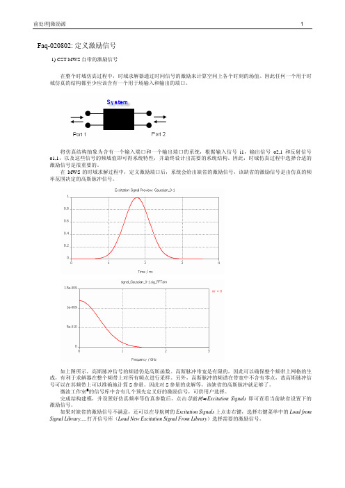
Faq-020802: 定义激励信号1) CST MWS自带的激励信号在整个时域仿真过程中,时域求解器通过时间信号的激励来计算空间上各个时刻的场值。
因此任何一个用于时域仿真的结构都至少应该含有一个用于场输入和输出的端口。
将仿真结构抽象为含有一个输入端口和一个输出端口的系统,根据输入信号i1,输出信号o2,1和反射信号o1,1,以及这些信号的频域值即可得系统特性,并最终设计出需要的系统结构。
因此,时域仿真过程中选择合适的激励信号是很重要的。
在MWS的时域求解过程中,定义激励端口后,系统会给出缺省的激励信号,该缺省的激励信号是由仿真的频率范围决定的高斯脉冲信号。
如上图所示,高斯脉冲信号的频谱仍是高斯函数。
高斯脉冲带宽是有限的,因此可以确保整个频带上网格的生成,有利于求解器在整个频带上对所有频点进行采样。
另外,高斯脉冲的频谱在带宽中不含有零点,故高斯脉冲信号可以在其频带上可以准确地计算S参量。
因此对S参量的求解等,该缺省的高斯脉冲就足够了。
微波工作室®的信号库中含有几个预先定义好的激励信号,可供用户选择。
完成结构建模,并设置好仿真频率等仿真参数后,点击导航树ÖExcitation Signals即可查看当前缺省设置下的激励信号。
如果对缺省的激励信号不满意,还可以在导航树的Excitation Signals上点击右键,选择右键菜单中的Load from Signal Library.....打开信号库(Load New Excitation Signal From Library)选择需要的激励信号。
在下图的信号库对话框中选择需要的激励信号后,点击Apply按钮即可完成信号的加载,在以后的仿真中,可以从求解器对话框中加载该信号对结构进行激励。
2) 自定义激励信号如果信号库中的信号都不能符合仿真要求,您还可以自己定义需要的激励信号。
完成结构建模,并设置好仿真频率等仿真参数后,在导航树的Excitation Signals上点击右键选择右键菜单中的New Excitation Signal......在打开的Excitation Signal对话框中选择Gaussian选项即可通过设定频率范围Fmin和Fmx来定义高斯脉冲信号,选择Rectangular选项即可通过指定信号的上升(Trise)、下降(Tfall)、保持(Thold)以及总激励时间(Ttotal)来定义矩形脉冲信号,并可以在Name栏中为定义的激励信号指定一个您喜欢的名字,这里我们定义一个矩形脉冲,并将名字命名为rectangular。
CST激励源之波导端口

CST激励源之波导端口波导端口是一种特殊种类的解算域边界条件,它可以刺激能量的吸收,这一切都是是通过2D频域解算器求解二维端口面内可能本征模实现的,且端口处每种可能的电磁场解析解都可以通过无数模式的叠加求得,然而,实际上,少量的模式就可以进行场仿真了,求解计算中需要考虑的模式数可以在Waveguide Port对话框中设定。
这里要注意:激励波导端口的输入信号是规一化到峰值功率为1 sqrt(Watt)使用波导端口要根据不同需求、不同特点的端口类型的数量定义。
因而,我们首先必须精确的判定激励问题的类型,然后在选择并定义合适的波导端口。
在具有不均匀性、可获得broadband ports(宽带端口)或者具有inhomogeneous port accuracy enhancement(非均匀端口精度加密)特色的情况下,我们可以选择使用normal waveguide ports(标准波导端口),与此同时,multipin ports可以计算凋落的TEM模。
标准波导端口标准波导端口即我们经常使用的矩形或圆形波导结构,通过PEC边界条件屏蔽,因而端口模式就被限制在端口区域内均匀波导端口右图是一个均匀、矩形标准波导端口,通过normalwaveguide operator解算。
下图中是一个具有三个模式的波导端口,这里按各自的截止频率来分类。
传播模式数的多少取决于选取的频率范围。
在瞬态仿真时,建议考虑所有的传播模式,因为未考虑的模式将在端口处引起反射。
对于凋落模式也采用同样的考虑,如果必要的话,求解器将检查这些情况并给出警告信息。
非均匀波导端口如果波导由两种或两种以上材料的介质填充如右图所示,那么模式就呈现频率依赖性,如下图所示就是三个不同频点的TE模,频率越高(从左到右频率逐渐增加),那么场就更加集中在具有高介电常数值的材料中(图中浅褐色部分所示)。
因为标准的波导解算器只计算指定频点处的场模式,对于宽带内计算场模式将会报错。
CST-VBA程序化建模(附实例解析)

3 VBA基础实例(零基础入门)
零基础入门:宏命令一键生成圆柱体周期阵列 VBA一键生成圆柱体周期阵列(将以上三段程序分别顺序粘贴
到空白程序的main函数内部即可,如下)
可用上述的两种方法重建物体: VBA命令框中点击Run Run Macro 中点击Cylinder_array
12
4 VBA进阶实例(参数化)
参数化建模:长方体周期阵列
参数定义
创建空白宏命令 写入宏命令代码
高 宽 长 间距 数量
运行宏命令,得到模型
13
4 VBA进阶实例(参数化)
参数化建模:长方体周期阵列(宏命令解析)
注释:’Box_Array 定义变量: Dim x As double 给物体命名: BrickName=“box1_”+Str(n) 【这样物体的名称为box1_ n,
消除空格的命令为: BrickName=“box1_”+LTrim(Str(n))】 关键:长方体的位置BrickX1等需用参数和n表征 合并物体: Solid.Add "component1:"+BrickName(1), "component1:"+BrickName(n)
14
5 VBA进阶实例(函数调用)
6
2 开启VBA之路
VBA宏进阶:创建空白宏命令
创建空白VBA命令,so easy!
7
2 开启VBA之路
VBA宏进阶:操作宏命令
点击它,直接生成物体 像CST自带宏命令一样运行 运行VBA宏命令的第二种方法
修改,Edit 其他CST程序也能
打开该宏命令,To Global 不想要了,delete
CST宏讲解

Examples OverviewThe usage of the VBA macro language is described in detail in the printed documentation "Advanced topics".Here are some typical examples to get in touch with the CST MICROWAVESTUDIO® VBA language:General• How to use the VBA Objects in general.Modelling:• Create analytical 2D curve.• Create analytical 3D curve.Solver and Post processing• Accessing S-Parameter Phase.• Calculating the real part of S11 at a certain frequency.• Define an excitation function.• Adding user defined entries to the result tree.• Creating 3D scalar and vector plots:• Create a farfield array.How to use the VBA ObjectsExample 1: Call CST MICROWAVE STUDIO™ from within an external application Creates a CST MICROWAVE STUDIO™ Application Object, opens a project and creates a brick:dim app as Object‘Starts the CST MICROWAVE STUDIO™set app = CreateObject(”MWStudio.Application”)app.OpenFile(”c:Exampleswg.mod”)dim br as Objectset br = CreateObject(”MWStudio.Brick”)With br.Reset.Name "BrickOne".Layer "default".Xrange "0", "1".Yrange "0", "2".Zrange "0", "4".CreateEnd WithExample2: Open a file within the build-in VBA interpreterOpens a project from the VBA-Interpreter of the CST MICROWAVE STUDIO™: OpenFile(”c:Exampleswg.mod”)With br.Reset.Name "BrickOne".Layer "default".Xrange "0", "1".Yrange "0", "2".Zrange "0", "4".CreateEnd WithCreate an anayltical 2D curve'--------------------------------------------------' arbitrary xy-function is converted into a curve'--------------------------------------------------Sub Main ()On Error GoTo Curve_ExistsCurve.NewCurve "2D-Analytical"Curve_Exists:On Error GoTo 0Dim sCurveName As StringBeginHideDim iii As Integeriii = 1While SelectTreeItem("Curves2D-Analyticalspline_"+CStr(iii))iii = iii+1WendsCurveName = "spline_"+CStr(iii)assign "sCurveName"EndHideWith Spline.Reset.Name sCurveName.Curve "2D-Analytical"' ======================================' !!! Do not change ABOVE this line !!!' ======================================' -----------------------------------------------------------' adjust x-range as for-loop parameters (xmin,max,stepsize)' enter y-Function-statement within for-loop' fixed parameters a,b,c have to be declared via Dim-Statement' -----------------------------------------------------------' NOTE: available MWS-Parameters can be used without' declaration at any place (loop-dimensions, ...)' (for parametric curves during parameter-sweeps and optimisation !) ' -------------------------------------------Dim xxx As Double, yyy As DoubleDim aaa As Double ' not necessary if aaa is model parameteraaa = 1.23456/Atn(0.5)For xxx = 1.5 To 10 STEP 0.5yyy = 3*aaa/xxx + Sin(xxx^2).LineTo xxx , yyyNext xxx' ======================================' !!! Do not change BELOW this line !!!' ======================================.CreateEnd WithSelectTreeItem("Curves2D-Analytical"+sCurveName)End SubCreate an analytical 3D curve'--------------------------------------------------' arbitrary analytical xyz-function is converted into a curve'--------------------------------------------------Sub Main ()On Error GoTo Curve_ExistsCurve.NewCurve "3D-Analytical"Curve_Exists:On Error GoTo 0Dim sCurveName As StringBeginHideDim iii As Integeriii = 1While SelectTreeItem("Curves3D-Analytical3dpolygon_"+CStr(iii))iii = iii+1WendsCurveName = "3dpolygon_"+CStr(iii)assign "sCurveName"EndHideWith Polygon3D.Reset.Name sCurveName.Curve "3D-Analytical"' ======================================' !!! Do not change ABOVE this line !!!' ======================================' -----------------------------------------------------------' adjust x-range as for-loop parameters (xmin,max,step)' enter y/z-Function-statement within for-loop' fixed parameters a,b,c have to be declared via Dim-Statement' -----------------------------------------------------------' NOTE: available MWS-Parameters can be used without' declaration at any place (loop-dimensions, ...)' (for parametric curves during parameter-sweeps and optimisation !)' -------------------------------------------Dim xxx As Double, yyy As Double, zzz As DoubleDim aaa As Double ' not necessary if aaa is model parameteraaa = 0.3For xxx = Pi/2 To 10*2*Pi STEP 0.2yyy = Sqr(2*Abs(Cos(xxx))) + 3*aaa/xxx + 2*Sin(xxx)zzz = Abs(yyy) - Sqr(2*Abs(Cos(xxx))) + 3*aaa/xxx + 2*Sin(xxx).Point Sin(xxx) , Cos(xxx) , aaa*xxxNext xxx' ======================================' !!! Do not change BELOW this line !!!' ======================================.CreateEnd WithSelectTreeItem("Curves3D-Analytical"+sCurveName)End SubAccessing S-Parameter PhaseExample 1: Accessing all values of S-Parameter phase, stored in file ^p1(1)1(1).sig With Result1D ("p1(1)1(1)") ‘ Connect to phase of S11nn = .GetN ‘ Get number of frq-pointsFor ii = 0 To nn-1' Read all points; index of first point is zero.v x = .GetX(ii) ‘ here: frequencyvy = .GetY(ii) ‘ here: according phaseNext iiEnd WithCalculating the real part of S11 at a certain frequencyCalculating the real part of S11 at a certain frequency (here 0.65 GHz)Dim a11 As ObjectDim p11 As ObjectSet a11 = Result1D ("a1(1)1(1)")Set p11 = Result1D ("p1(1)1(1)")Dim n As IntegerDim frq As Doublefrq=0.65n=a11.GetClosestIndexFromX(frq)phase = Pi/180.0 * p11.GetY(n)ampli = a11.GetY(n)real = ampli * cos(phase)ResultTree ExamplesThe ResultTree VBA Object offers very interesting possibilities to configure the Navigation Tree. It is possible to insert different simulation results as well as VBA macros. The following examples will show its functionality.Examples to add Signal Views into the treeAll following examples add items into the folder ”My S-Parameters”. If this folder does not exist it will be created.For inserting signals into the tree it is possible to import results from other projects. Therefore the complete result file name must be specified with the File method. If the results of the current project shall be inserted, the project name in the result file name may be omitted.Signal into Tree 1: Adds a linear view of the amplitude of an extern S11 S-Parameter into the folder.Signal into Tree 2: Adds a linear view of the phase of an extern S11 S-Parameter into the folder.Signal into Tree 3: Adds a Smith Chart view of a S11 S-Parameter into the folder.Signal into Tree 4: Adds a Polar Plot of the S11 S-Parameter into the folder.Examples to add Field Plot Views into the treeFor results others than Signals only those of the current project can be inserted into the tree!Field Plot into Tree: Adds a 3D-Vector plot into the tree.Farfield into Tree: Adds a Farfield into the tree.Examples to add a macro into the treeEvery time a macro is executed from the tree, a VBA command interpreter is started and evaluates the string that has been set by the Macro method. Therefore no variables that are defined within the script that creates the folder entry can be accessed by the macro. Macro into Tree 1: Adds a command to start the time domain solver into the tree.Macro into Tree 2: Adds a macro into the tree.Macro into Tree 3: Adds an external VBA script into the tree.Signal into Tree 1Adds a linear view of the amplitude of the S11 S-Parameter from the project봂xtProj?into the folder. ExtProj is supposed to be located in the directory of the current project.With ResultTree.Reset.Name "My S-ParametersS11 (lin)" ' The entry name and its destination folder.Title "S11 (linear)" ' Title of the plot.File "ExtProj^a1(1)1(1).sig" ' The name of the signal file.Type "XYSignal" ' Plot Type.XLabel "f/Hz" ' Label for the x-axis.Subtype "Linear" ' Sub Plot Type.AddEnd WithSee also: Result TreeSignal into Tree 2Adds a linear view of the phase of the S11 S-Parameter from the project 봂xtProj?into the folder. ExtProj is supposed to be located in the directory of the current project.With ResultTree.Reset' The entry name and its destination folder.Name "My S-ParametersS11 (phase)".Title "S11 (phase)" ' Title of the plot.File "ExtProj^p1(1)1(1).sig" ' The name of the signal file.Type "XYSignal" ' Plot Type.XLabel "f/Hz" ' Label for the x-axis.Subtype "Phase" ' Sub Plot Type.AddEnd WithSee also: Result TreeSignal into Tree 3Adds a Smith Chart view of the S11 S-Parameter from the current project into the folder.A value has to be given to which the values in the plot are normalized.With ResultTree.Reset' The entry name and its destination folder.Name "My S-ParametersS11 (Smith Chart)".Title "S11" ' Title of the plot.ReferenceImpedance "50" ' Impedance to which the Values' will be normalized' Result files with the amplitude and phase values.File "^a1(1)1(1).sig".File2 "^p1(1)1(1).sig".Type "SmithSignal" ' Type of the plot.AddEnd WithSee also: Result TreeSignal into Tree 4Adds a Polar Plot view of the S11 S-Parameter from the current project into the folder. With ResultTree.Reset' The entry name and its destination folder.Name "My S-ParametersS11 (polar)"' Result files with the amplitude and phase values.File "^a1(1)1(1).sig".File2 "^p1(1)1(1).sig".Type "PolarSignal" ' Type of the plot.AddEnd WithField Plot into TreeAdds a Field Plot view of the electric field from the current project into the folder ”MyFieldView”.With ResultTree' The entry name and its destination folder.Name "My FieldViewE_Field".File "^e1_1.m3d" ' Result file name.Type "Efield3D" ' Entry type.AddEnd WithFarfield into TreeAdds a Farfield Plot view from the current project into the folder 봎y FieldView?With ResultTree' The entry name and its destination folder.Name "My FieldViewFarfield".File "^ff1_1.ffm" ' Result file name.Type "Farfield" ' Entry type.AddEnd WithMacro into Tree 1Adds a command into the 봘serdefined?folder that starts the time domain solver.With ResultTree' The entry name and its destination folder.Name "UserdefinedMacro1"' String to be evaluated by the VBA Interpreter.Macro "Solver.Start".Type "Macro" ' Entry type.AddEnd WithMacro into Tree 2Adds the pr eviously defined control macro ”AutoTest” into the tree.At first a string will be defined that contains a VBA command that executes the control macro. The command is ”RunMacro” that takes a string (the name of the control macro) as its argument. However, strings have to be specified within quotes. Unfortunately quotes are special characters which are not recognized as normal characters. They mark the start and the end of a string. Therefore the variable a is defined with a single quote as its only content. With this quote the entire command string can be constructed.Dim a As Stringa = """a = "RunMacro " & a & "AutoTest" & a' a contains the string: RunMacro "AutoTest"With ResultTree' The entry name and its destination folder.Name "UserdefinedMacro2"' String to be evaluated by the VBA Interpreter.Macro a.Type "Macro" ' Entry type.AddEnd WithMacro into Tree 3Adds an external VBA script into the tree. Let the name of the external macrobe ”Macro1.bas” that will be located in the directory of t he current project.At first a string will be defined that contains a VBA command that executes an external VBA script file. The command is ”MacroRun” that takes a string (the name of t he script) as its argument. However, strings have to be specified within quotes. Unfortunately quotes are special characters which are not recognized as normal characters. They mark the start and the end of a string. Therefore the variable a is defined with a single quote as its only content. With this quote the entire command string can be constructed.Dim a As Stringa = """a = "MacroRun " & a & "Macro1.bas" & a' a contains the string: MacroRun "Macro1.bas"With ResultTree' The entry name and its destination folder.Name "UserdefinedMacro3"' String to be evaluated by the VBA Interpreter.Macro a.Type "Macro" ' Entry type.AddEnd WithScalarPlot3D ExampleThe following script plots surfaces of equal amplitude of the vector field component Y of the electric field ”e1”.‘ Plot only a wire frame of the structure to be able to look insidePlot.wireframe True‘ Select the Y-Component of the electric field e1 in the treeSelectTreeItem ("2D/3D ResultsE-Fielde1Y")‘ Plot the scalar field of the selecte d monitorWith ScalarPlot3D.Type "isosurfaces".PlotAmplitude False.Scaling 50.LogScale False.ContourLines False.ScaleToVectorMaximum True.Quality 60.PlotEnd WithSee Also: SelectTreeItem, PlotVectorPlot3D ExampleThe following script plots the electric field ”e1” (if available) in a linear scale by using 400 colored arrows.‘ Plot only a wire frame of the structure to be able to look insidePlot.wireframe True‘ Select the desired monitor in the tree.SelectTreeItem ("2D/3D ResultsE-Fielde1")‘ Plot the field of the selected monitorWith VectorPlot3D.Type "arrowscolor".Objects 400.Scaling 50.LogScale False.PlotEnd WithSee Also: SelectTreeItem, PlotFarfieldArray ObjectGroup: PostprocessingDescription: Defines the antenna array pattern for a farfieldplot based on a single antenna element.Methods: Reset , UseArray , Arraytype , XSet , YSet , Zset , SetList , DeleteList , AntennaFunctions: noneExample:With FarfieldArray.Reset.UseArray "True".Arraytype "Rectangular".ZSet "2", "2,5", "90".SetList.Arraytype "Edit".Antenna "0", "0", "0", "1.0", "0"End With。
CST VBA的使用方法
4
| Oct-07
Integration Into Workflow
MS Windows Scripting Host COM DCOM Excel, Word, Matlab, AutoCad, etc...
e.g. ppt-Reports
reports
e.g. bidirectional Excel link
Returns a value
21
| Oct-07
Outline
Why macro programming? Existing macros Different types of macros Creating and testing new macros Getting more information
CST STUDIO SUITE‘s macro language: Compatible to the widely used VBA (Visual Basic for Applications) COM based CST STUDIO SUITE can be controlled by other applications CST STUDIO SUITE can control other applications
Execute command in Matlab
CST MWS is called Path of the VBA script within the CST DESIGN Sub Main ENVIRONMENT Opens an existing CST MWS file OpenFile("D:\MBK\test1\test1.mod") Solver.Start Start of Transient Solver Save End Sub Saves results and gives control back to Matlab
CST使用教程(14)设置平面波激励2024新版

平面波是理想化的模型,在实际情况中,由于各种因素的影响,如衍射、 散射等,完美的平面波并不存在。
平面波激励原理介绍
1
平面波激励是一种在电磁仿真中常用的激励方式 ,用于模拟电磁波在自由空间或特定媒质中的传 播。
2
在CST中,平面波激励通过设置波的传播方向、 极化方式、频率等参数,可以模拟不同条件下的 电磁波传播情况。
01
建模步骤
02
定义材料属性和几何尺寸;
03 设置边界条件和载荷,包括平面波激励的幅值、 频率和方向;
案例一:简单结构平面波激励分析
查看结构的位移、应力和 应变分布;
结果分析
划分网格并进行求解。
01
03 02
案例一:简单结构平面波激励分析
分析不同频率下结构的响应特性;
评估结构的动态性能。
案例二:复杂结构平面波激励分析
部分。
菜单栏提供了软件的所有功能选项, 如文件操作、编辑、视图、仿真、结
果等。
工具栏提供了常用功能的快捷按钮, 方便用户快速访问。
项目树展示了当前仿真的所有相关文 件和设置,用户可以通过项目树进行 快速导航和编辑。
属性窗口用于显示和编辑当前选中对 象的属性,如材料、边界条件、激励 等。
仿真窗口用于显示仿真结果和进行后 处理操作,如数据可视化、动画演示 等。
02
在CST中,设置平面波激励可以模拟天线、滤波器、耦合器等电
磁器件的性能。
提升仿真效率
03
通过合理设置平面波激励,可以提高仿真的准确性和效率。
教程范围
基本概念介绍
简要介绍平面波激励的定义、特点及其在电磁仿 真中的应用。
CST MS2010 L3 有关激励、线缆和电路元件
电路端口
• 共面波导端口 Co-Planar;
– 点选共面波导各 金属结构的端面 (如果有厚度) 或者端线(如果 是二维面) – 端口的参考面 (垂直于共面波 导,图中红色框 所示)扩展到整 个求解域
用户定义端口
• 激励信号入射方向 Ingoing Direction • 例:内嵌微带端口的设 定
27
CST MS培训教程 L3 有关激励、线缆和电路元件
CST China Ltd | | info@
用户定义端口
• 某些情况下,需要将馈电点嵌入到结构中 去
CST China Ltd | | info@
内容提要
• 模型是如何被激励的 • 激励的类型:
– 端口激励
• 可能是最常用的激励方式
– 使用线缆和电路器件 – 平面波激励
3
CST MS培训教程 L3 有关激励、线缆和电路元件
CST China Ltd | | info@
可以灵活指定波导的激励模式,同时 软件会自动计算出该模式下的截止频 率
15 CST MS培训教程 L3 有关激励、线缆和电路元件 CST China Ltd | | info@
波导端口
• 非标准波导端口:
– 应用于脊波导、双脊波导、介质加载等。 – MICROSTRIPES 不会自动的判断出该端口 为非标准的波导端口。 – 求解器通过在前处理中设定的截止频率来 判断并求解非标准波导端口。
• 两种主要类型:
– 波导端口 – 电路端口
• ‘一击’设定:
– 激励源 – 输出参量 – 终端端接
CST_VBA界面的创建
第二章 VBA创建界面VBA采用VB的编程语言和语法,是一种可视化的、面向对象的、采用事件驱动的结构化高级程序设计语言,不过VBA的部分函数与VB的不一样,这一点需要注意。
一个完整的VBA程序通常包含以下几个部分:①界面。
界面也就是人机对话框,用户可以通过输入相关数据、点击操作按钮,让VBA进行各种数据计算、模型创建、数据输出等功能。
②主程序。
主程序也就是Sub Main和End Sub之间的程序,主程序可以实现宏文件的特定功能,是一个完整的程序体。
③子程序。
子程序可以完成某个具体的小功能,是为主程序服务的。
有时候主程序需要反复执行同一操作,若每次都编写同样的程序,则显得过于冗杂。
因此编写功能很小、但很具体的子程序,可以随时调用。
④数据输出。
有的时候,经过计算的数据需要输出到txt文件、打印成报表格式等,因此程序中还应该具备数据输出的功能。
当然,该功能是附属功能,可以不存在。
如果一个宏程序中包含了上述四个部分,那么该宏程序就是一个非常完整、功能齐全的程序了。
接下来首先讲解如何利用VBA创建界面。
在CST主窗口的菜单栏中打开Open VBA Macro Editor,单击图1-9左侧的图标,那么就打开了窗口编辑对话框,如图2-1所示。
图2-1 窗口编辑对话框之前使用过VB软件的可能会发现,VBA此时的操作界面竟然和VB的操作界面一模一样,都具备可视化的效果。
图2-1左侧部分是窗体中可以使用的控件,包括text文本框、单选按钮等等,中部是放置控件的载体,它的大小可以任意调整,而调整后的大小就是实际的窗体大小。
需要注意的是:创建的窗体中必须至少包含OKButton和CancelButton 中的一个,否则系统会提示存在错误。
2.1 控件① Text静态文本静态文本text通常用来显示数据输出,或者提示用户的标签等。
在窗体中添加一个静态文本,双击便可打开并查看text1静态文本的部分属性,如图2-2所示。
VBA简介
第一章 VBA简介Visual Basic for Applications(VBA)是一种Visual Basic的一种宏语言,提供了面向对象的程序设计方法,相当完整的程序设计过程,是一种可视化的、面向对象的、采用事件驱动的结构化高级程序设计语言。
它具有高效率、简单易学及功能强大的特点。
此处要介绍的VBA是在CST仿真软件中编写宏语言的,编写的宏可以完成某一指定的具体任务,如人机对话框、数据处理、联合建模并仿真等等。
1.1 VBA运行环境首先打开CST仿真软件,单击菜单栏的Macros选项,将会弹出如图1-1所示的界面。
图1-1 CST界面下的Macros菜单界面图1-1的界面中红色圆圈圈出的部分有五个选项,分别是Open VBA MacroEditor、Make VBA Macro...、Import VBA Macro...、Edit/Move/Delete VBA Macro…、Set Global Macro Path,这五个选项具备不同的功能。
① Open VBA Macro Editor当用户打开VBA宏编辑器,就可以在该界面中编辑新的VBA宏。
该界面不存在任何的模板程序,完全需要用户自己往里面书写程序,该界面示意图如图1-2所示。
通常情况下,该种方法使用较多。
注意:Sub Main和End Sub分别是宏的开始和结束,因此用户编写的宏程序必须在Sub Main和End Sub之间。
图1-2 打开VBA宏编辑器的界面② Make VBA Macro...当打开Make VBA Macro...选项的时候,会弹出图1-3所示的对话框。
在Macro 中输入新创建宏的名字。
接下来选择创建宏的性质——Control Macro 和Structure Macro,他们都是工程宏,也就是他们是只属于此CST工程,在其他CST 工程中将不能使用,如果选择了Make globally available复选框,那么创建的宏则是属于全局宏,可以在任意的CST工程中使用。
CST中的激励源
微波技术网、微波家园共同打造微波社区门户网站
http://i微m波w.技m术w网
带有接地平面的两个导体微带线 下图给出带有接地平面的两个导体微带线的奇模、偶模分布,由于端口区域的不连续性,其 奇偶模都是非退化的 QTEM(准 TEM 波),描绘了这种结构的两种静态模式。
参数结果,请注意:端口编号是和离散端口 discrete port 的定义共享的(一致的)
Normal:选择端口面的法向。端口必须平行于计算域的边界以便你可以在 x、y、z 之间选择。 Orientation:定义端口的方向,如辐射方向。Lower 端
口辐射方向为正方向,upper 端口辐射方向为负方向,
微波技术网、微波家园共同打造微波社区门户网站
http://i微m波w.技m术w网
均匀同轴波导或同轴连接器端口 右图中的均匀同轴波导由一个外导体和四个内导体构成,
因此存在三个不同 TEM 模式,如下图所示。这些模式是凋落模 (具有相同的传播常数),且可以叠加产生新的模式,这是因为 他们彼此是正交的。因此,下图所示的模式解仅仅是一种可 能解,因而我们建议你使用 multipin operator 功能指定你 期望激励的模式。
波导端口 波导端口是根据入射波功率和反射波功率来进行求解计算的,对每个波导端口而言,在计算 求解过程中,都将记录其 S 参数(时域信号用于时域仿真)。实际上,端口可以被连接到结构 中的纵向均匀波导代替。在仿真求解前,你至少需要一个激励源(或波导端口、或离散端口 或平面波)对结构进行馈电。 注:激励的波导端口的输入信号是规一化到 1 sqrt(watt)的。
- 1、下载文档前请自行甄别文档内容的完整性,平台不提供额外的编辑、内容补充、找答案等附加服务。
- 2、"仅部分预览"的文档,不可在线预览部分如存在完整性等问题,可反馈申请退款(可完整预览的文档不适用该条件!)。
- 3、如文档侵犯您的权益,请联系客服反馈,我们会尽快为您处理(人工客服工作时间:9:00-18:30)。
Faq-020802: 定义激励信号
1) CST MWS自带的激励信号
在整个时域仿真过程中,时域求解器通过时间信号的激励来计算空间上各个时刻的场值。
因此任何一个用于时域仿真的结构都至少应该含有一个用于场输入和输出的端口。
将仿真结构抽象为含有一个输入端口和一个输出端口的系统,根据输入信号i1,输出信号o2,1和反射信号o1,1,以及这些信号的频域值即可得系统特性,并最终设计出需要的系统结构。
因此,时域仿真过程中选择合适的激励信号是很重要的。
在MWS的时域求解过程中,定义激励端口后,系统会给出缺省的激励信号,该缺省的激励信号是由仿真的频率范围决定的高斯脉冲信号。
如上图所示,高斯脉冲信号的频谱仍是高斯函数。
高斯脉冲带宽是有限的,因此可以确保整个频带上网格的生成,有利于求解器在整个频带上对所有频点进行采样。
另外,高斯脉冲的频谱在带宽中不含有零点,故高斯脉冲信号可以在其频带上可以准确地计算S参量。
因此对S参量的求解等,该缺省的高斯脉冲就足够了。
微波工作室®的信号库中含有几个预先定义好的激励信号,可供用户选择。
完成结构建模,并设置好仿真频率等仿真参数后,点击导航树ÖExcitation Signals即可查看当前缺省设置下的激励信号。
如果对缺省的激励信号不满意,还可以在导航树的Excitation Signals上点击右键,选择右键菜单中的Load from Signal Library.....打开信号库(Load New Excitation Signal From Library)选择需要的激励信号。
在下图的信号库对话框中选择需要的激励信号后,点击Apply按钮即可完成信号的加载,在以后的仿真中,可以从求解器对话框中加载该信号对结构进行激励。
2) 自定义激励信号
如果信号库中的信号都不能符合仿真要求,您还可以自己定义需要的激励信号。
完成结构建模,并设置好仿真频率等仿真参数后,在导航树的Excitation Signals上点击右键选择右键菜单中的New Excitation Signal......
在打开的Excitation Signal对话框中选择Gaussian选项即可通过设定频率范围Fmin和Fmx来定义高斯脉冲信号,选择Rectangular选项即可通过指定信号的上升(Trise)、下降(Tfall)、保持(Thold)以及总激励时间(Ttotal)来定义矩形脉冲信号,并可以在Name栏中为定义的激励信号指定一个您喜欢的名字,这里我们定义一个矩形脉冲,并将名字命名为rectangular。
完成激励信号的设置后,点击OK按钮关闭对话框,即可在导航树中打开Excitation Signals文件夹,选择rectangular选项查看添加的激励信号。
选择User defined选项,将激活Edit.....。
点击该按钮即进入VBA编辑器。
在打开的VBA编辑器中您可以利用相应的VBA命令来定义需要的激励信号。
系统已经帮您定义好激励函数Function ExcitationFunction(dtime As Double) As Double您可以在该激励函数中利
2π的正弦函数。
用VBA命令定义需要的激励信号。
例如,我们在这里定义一个0到
在激励函数ExcitationFunction中输入正弦函数语句,如下图所示:
回到主视图中界面将Excitation Signal对话框中的Ttotal变为2*pi,并为该信号指定一个您喜欢的名字(这里我们定义为sin_func),点击OK按钮即完成激励信号的定义。
此时,导航树会自动指向新定义的激励信号sin_func。
至此,您已经成功地完成了激励信号的定义和加载,可以在随后的仿真中指定该信号对端口进行激励。
另外:为了方便您对编写的VBA激励信号进行调试查看,系统还预先定义好主函数Sub Main2。
例如,我们需要对VBA命令编写正弦激励信号进行调试查看,将其变为sin(x)*cos(x)则需要进行以下操作:(1)回到VBA编辑器界面,将主函数中的Sub Main2变为Sub Main,把最长激励时间tmax由缺省的10.0变为2*pi。
并且让激励信号函数Function ExcitationFunction=sin(x)*cos(x)
(2)点击Run Macro按钮,运行该程序。
(3)程序运行后,回到主视图中。
此时,导航树自动指向Excitation Signals->Userdefined Functions->sin_func_plot,此函数即是新定义的激励信号。
(4)激励信号符合要求后,请一定回到VBA编辑器界面,将主函数Sub Main更名为Sub Main2等其他的名字,并保存程序。
(5)、最后回到主视图中,点击Excitation Signal对话框中的OK按钮,关闭对话框,即成功完成信号的定义和加载,在以后的仿真中可以选择sin_func、rectangular或是default作为激励信号。
注意:主函数Sub Main只做调试用,故完成信号定义前一定要将其更名为Sub Main2等其他的名字。
如果您保持主程序Sub Main的名字不变,则激励信号sin_func将仍是调试以前定义的信号。
恭喜您!您现在已经可以在微波工作室®中随意定义需要的激励信号了!。