Functional time series 函数时间序列
专业英文词汇表

专业英文词汇表以下是一些常见的专业英文词汇表,按字母顺序排列:AAbstract 摘要Analysis 分析Assessment 评估Algorithm 算法Architecture 架构Academic 学术的Application 应用Algorithmic 算法的Artificial intelligence 人工智能Automation 自动化BBenchmark 基准Backward compatibility 向后兼容性Big data 大数据Biotechnology 生物技术Business intelligence 商业智能CComputing 计算机科学Cryptography 密码学Component 组件Computer graphics 计算机图形学Control system 控制系统Cybersecurity 网络安全DData 数据Database 数据库Design 设计Development 开发Digital 数字化Distributed system 分布式系统EEncryption 加密Ethics 伦理学Engineering 工程学Experiment 实验Expert system 专家系统FFramework 框架Functional programming 函数式编程Genetic algorithm 遗传算法Grid computing 网格计算HHardware 硬件Hypothesis 假设Human-computer interaction 人机交互Hierarchical clustering 分层聚类IInformation technology 信息技术Interface 接口Internet of Things 物联网Image processing 图像处理JJava programming language Java编程语言KKnowledge 知识Knowledge management 知识管理LLogic logicLinguistics 语言学Linear programming 线性规划MMachine learning 机器学习Modeling 建模Machine vision 机器视觉Microprocessor 微处理器Multimedia 多媒体NNetwork 网络Neural network 神经网络OObject-oriented programming 面向对象编程Operating system 操作系统Optimization 优化Open-source 开源PProgramming programmingParallel computing 并行计算Quality assurance 质量保证Protocol 协议QQuery 查询RRobotic 嵌入式Robotics 机器人技术Random access memory (RAM) 随机存取存储器SSimulation 模拟Software 软件Systematic system 系统化System 系统Statistical analysis 统计分析Security 安全Storage 存储TTesting 测试Technology 技术Telecommunication 通信Theory 理论Transaction 事务Time series 时间序列Turing machine 图灵机UUser interface 用户界面Undo 撤销VVirtual reality 虚拟现实Validation 验证Visualization 可视化WWeb development 网络开发Wireless 无线XXML (Extensible Markup Language) 可扩展标记语言YYield rate 产率ZZero-day vulnerability 零日漏洞。
时间序列 (Time series)
时间序列①shapelets: 这种新技术允许准确、快速识别和分类①时间序列是指将某种现象某一个统计指标在不同时间上的各个数值,按时间先后顺序排列而形成的序列。
摘要:在过去几十年中,分类时间序列被吸引了的极大的兴趣。
虽然提出了几十个技术,但是最近的实证证据强烈的显示简单的最近邻算法②是非常困难的对于大多数时间序列击败问题,特别是大规模数据集。
然而这种方式会被认为是好消息,因为简单的实施最近的邻近算法,有一些负面影响。
第一,最近邻算法需要存储和检索整个数据集,导致在一个高度的时间和空间上这就限制了它的适用复杂度,特别是在资源有限的传感器上。
第二,超越分类精度,我们常常希望获得的洞察力数据,使分类结果更易理解,总体的最临近算法特点不能提供的。
在这篇论文中,我们介绍一种新的时间序列模型(元素)、时间序列shapelets系列,处理这些限制。
一般来说,shapelets是时间序列结果,在某种意义上,最大限度地代表性的类。
我们可以用shapeslet的距离,而不是距离到最近的邻居分类的对象。
我们将展示广泛的实证评价在不同的领域,分类算法通过时间序列shapelet元素可以被更易识别的,更准确,速度快得多的分类。
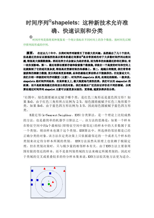
②右图中,绿色圆要被决定赋予哪个类,是红色三角形还是蓝色四方形?如果K=3,由于红色三角形所占比例为2/3,绿色圆将被赋予红色三角形那个类,如果K=5,由于蓝色四方形比例为3/5,因此绿色圆被赋予蓝色四方形类。
K最近邻(k-Nearest Neighbor,KNN)分类算法,是一个理论上比较成熟的方法,也是最简单的机器学习算法之一。
该方法的思路是:如果一个样本在特征空间中的k个最相似(即特征空间中最邻近)的样本中的大多数属于某一个类别,则该样本也属于这个类别。
KNN算法中,所选择的邻居都是已经正确分类的对象。
该方法在定类决策上只依据最邻近的一个或者几个样本的类别来决定待分样本所属的类别。
KNN方法虽然从原理上也依赖于极限定理,但在类别决策时,只与极少量的相邻样本有关。
matlab时间序列的多时间尺度小波分析
小波分析—时间序列的多时间尺度分析一、问题引入1.时间序列(Time Series )时间序列是指将某种现象某一个统计指标在不同时间上的各个数值,按时间先后顺序排列而形成的序列。
在时间序列研究中,时域和频域是常用的两种基本形式。
其中:时域分析具有时间定位能力,但无法得到关于时间序列变化的更多信息;频域分析(如Fourier 变换)虽具有准确的频率定位功能,但仅适合平稳时间序列分析。
然而,许多现象(如河川径流、地震波、暴雨、洪水等)随时间的变化往往受到多种因素的综合影响,大都属于非平稳序列,它们不但具有趋势性、周期性等特征,还存在随机性、突变性以及“多时间尺度”结构,具有多层次演变规律。
对于这类非平稳时间序列的研究,通常需要某一频段对应的时间信息,或某一时段的频域信息。
显然,时域分析和频域分析对此均无能为力。
2.多时间尺度河流因受季节气候和流域地下地质因素的综合作用的影响,就会呈现出时间尺度从日、月到年,甚至到千万年的多时间尺度径流变化特征。
推而广之,这个尺度分析,可以运用到对人文历史的认识,以及我们个人生活及人生的思考。
3.小波分析产生:基于以往对于时间序列分析的各种缺点,融合多时间尺度的理念,小波分析在上世纪80年代应运而生,为更好的研究时间序列问题提供了可能,它能清晰的揭示出隐藏在时间序列中的多种变化周期,充分反映系统在不同时间尺度中的变化趋势,并能对系统未来发展趋势进行定性估计。
优点:相对于Fourier 分析:Fourier 分析只考虑时域和频域之间的一对一的映射,它以单个变量(时间或频率)的函数标示信号;小波分析则利用联合时间-尺度函数分析非平稳信号。
相对于时域分析:时域分析在时域平面上标示非平稳信号,小波分析描述非平稳信号虽然也在二维平面上,但不是在时域平面上,而是在所谓的时间尺度平面上,在小波分析中,人们可以在不同尺度上来观测信号这种对信号分析的多尺度观点是小波分析的基本特征。
应用范围:目前,小波分析理论已在信号处理、图像压缩、模式识别、数值分析和大气科学等众多的非线性科学领域内得到了广泛的应用。
数学专业词汇
数学专业词汇Aabsolute value 绝对值 accept 接受 acceptable region 接受域additivity 可加性adjusted 调整的alternative hypothesis 对立假设analysis 分析 analysis of covariance 协方差分析 analysis of variance 方差分析 arithmetic mean 算术平均值association 相关性assumption 假设assumption checking 假设检验 availability 有效度average 均值Bbalanced 平衡的band 带宽bar chart 条形图beta-distribution 贝塔分布 between groups 组间的 bias 偏倚 binomial distribution 二项分布 binomial test 二项检验Ccalculate 计算 case 个案 category 类别 center of gravity 重心 central tendency 中心趋势 chi-square distribution 卡方分布 chi-square test 卡方检验 classify 分类 cluster analysis 聚类分析coefficient 系数coefficient of correlation 相关系数collinearity 共线性column 列compare 比较comparison 对照components 构成,分量compound 复合的confidence interval 置信区间consistency 一致性 constant 常数continuous variable 连续变量control charts 控制图correlation 相关covariance 协方差 covariance matrix 协方差矩阵 critical point 临界点critical value 临界值 crosstab 列联表cubic 三次的,立方的 cubic term 三次项 cumulative distribution function 累加分布函数 curve estimation 曲线估计Ddata 数据default 默认的definition 定义deleted residual 剔除残差density function 密度函数 dependent variable 因变量 description 描述 design of experiment 试验设计deviations 差异df.(degree of freedom) 自由度diagnostic 诊断 dimension 维 discrete variable 离散变量discriminant function 判别函数 discriminatory analysis 判别分析distance 距离distribution 分布D-optimal design D-优化设计Eeaqual 相等 effects of interaction 交互效应 efficiency 有效性eigenvalue 特征值 equal size 等含量 equation 方程error 误差 estimate 估计 estimation of parameters 参数估计 estimations 估计量 evaluate 衡量 exact value 精确值expectation 期望 expected value 期望值 exponential 指数的 exponential distributon 指数分布 extreme value 极值F factor 因素,因子 factor analysis 因子分析 factor score 因子得分factorial designs 析因设计factorial experiment 析因试验 fit 拟合fitted line 拟合线 fitted value 拟合值 fixed model 固定模型 fixed variable 固定变量 fractional factorial design 部分析因设计 frequency 频数F-test F检验full factorial design 完全析因设计function 函数Ggamma distribution 伽玛分布geometric mean 几何均值group 组Hharmomic mean 调和均值 heterogeneity 不齐性histogram 直方图 homogeneity 齐性 homogeneity of variance 方差齐性hypothesis 假设 hypothesis test 假设检验Iindependence 独立independent variable 自变量independent-samples 独立样本index 指数index of correlation 相关指数interaction 交互作用interclass correlation 组内相关interval estimate 区间估计intraclass correlation 组间相关 inverse 倒数的iterate 迭代Kkernal 核 Kolmogorov-Smirnov test柯尔莫哥洛夫-斯米诺夫检验 kurtosis 峰度Llarge sample problem 大样本问题layer 层least-significant difference 最小显著差数 least-square estimation 最小二乘估计 least-square method 最小二乘法level 水平level of significance 显著性水平leverage value 中心化杠杆值life 寿命life test 寿命试验likelihood function 似然函数 likelihood ratio test 似然比检验 linear 线性的 linear estimator 线性估计linear model 线性模型linear regression 线性回归linear relation 线性关系 linear term 线性项 logarithmic 对数的logarithms 对数 logistic 逻辑的 lost function 损失函数Mmain effect 主效应 matrix 矩阵 maximum 最大值 maximum likelihood estimation 极大似然估计mean squared deviation(MSD) 均方差 mean sum of square 均方和 measure 衡量media 中位数M-estimator M估计minimum 最小值missing values 缺失值 mixed model 混合模型 mode 众数model 模型Monte Carle method 蒙特卡罗法 moving average 移动平均值multicollinearity 多元共线性multiplecomparison 多重比较multiple correlation 多重相关multiple correlation coefficient 复相关系数multiple correlation coefficient 多元相关系数 multiple regression analysis 多元回归分析 multiple regression equation 多元回归方程 multiple response 多响应 multivariate analysis 多元分析Nnegative relationship 负相关nonadditively 不可加性nonlinear 非线性nonlinear regression 非线性回归noparametric tests 非参数检验 normal distribution 正态分布 null hypothesis 零假设 number of cases 个案数Oone-sample 单样本 one-tailed test 单侧检验 one-way ANOVA 单向方差分析 one-way classification 单向分类 optimal 优化的optimum allocation 最优配制order 排序order statistics 次序统计量origin 原点orthogonal 正交的outliers 异常值Ppaired observations 成对观测数据 paired-sample 成对样本 parameter 参数parameter estimation 参数估计 partial correlation 偏相关partial correlation coefficient 偏相关系数 partial regression coefficient 偏回归系数 percent百分数percentiles 百分位数pie chart 饼图point estimate 点估计poisson distribution 泊松分布polynomial curve 多项式曲线 polynomial regression 多项式回归polynomials 多项式positive relationship 正相关power 幂P-P plot P-P概率图 predict 预测 predicted value 预测值 prediction intervals 预测区间 principal component analysis 主成分分析 proability 概率 probability density function 概率密度函数probit analysis 概率分析proportion 比例Qqadratic 二次的 Q-Q plot Q-Q概率图 quadratic term 二次项 quality control 质量控制 quantitative 数量的,度量的quartiles 四分位数Rrandom 随机的 random number 随机数 random number 随机数random sampling 随机取样 random seed 随机数种子 random variable 随机变量 randomization 随机化 range 极差 rank 秩rank correlation 秩相关rank statistic 秩统计量regression analysis 回归分析 regression coefficient 回归系数 regression line 回归线 reject 拒绝 rejection region 拒绝域 relationship 关系 reliability 可*性 repeated 重复的 report 报告,报表 residual 残差 residual sum ofsquares 剩余平方和 response 响应 risk function 风险函数robustness 稳健性 root mean square 标准差 row 行 run 游程 run test 游程检验Sample 样本 sample size 样本容量 sample space 样本空间sampling 取样 sampling inspection 抽样检验 scatter chart 散点图 S-curve S形曲线 separately 单独地 sets 集合 sign test 符号检验 significance 显著性 significance level 显著性水平 significance testing 显著性检验 significant 显著的,有效的significant digits 有效数字skewed distribution 偏态分布 skewness 偏度 small sample problem 小样本问题 smooth 平滑 sort 排序 soruces of variation 方差来源space 空间spread 扩展square 平方standard deviation 标准离差 standard error of mean 均值的标准误差standardization 标准化 standardize 标准化 statistic 统计量statistical quality control 统计质量控制std. residual 标准残差 stepwise regression analysis 逐步回归stimulus 刺激strong assumption 强假设stud. deleted residual 学生化剔除残差stud. residual 学生化残差subsamples 次级样本 sufficient statistic 充分统计量 sum 和 sum of squares 平方和 summary 概括,综述Ttable 表 t-distribution t分布 test 检验 test criterion 检验判据 test for linearity 线性检验 test of goodness of fit 拟合优度检验 test of homogeneity 齐性检验 test of independence 独立性检验test rules 检验法则test statistics 检验统计量testing function 检验函数time series 时间序列 tolerance limits 容许限 total 总共,和transformation 转换 treatment 处理 trimmed mean 截尾均值 true value 真值 t-test t检验 two-tailed test 双侧检验Uunbalanced 不平衡的unbiased estimation 无偏估计unbiasedness 无偏性 uniform distribution 均匀分布Vvalue of estimator 估计值 variable 变量 variance 方差variance components 方差分量variance ratio 方差比various 不同的 vector 向量Wweight 加权,权重 weighted average 加权平均值 within groups 组内的ZZ score Z分数2. 最优化方法词汇英汉对照表Aactive constraint 活动约束 active set method 活动集法analytic gradient 解析梯度 approximate 近似 arbitrary 强制性的 argument 变量 attainment factor 达到因子Bbandwidth 带宽 be equivalent to 等价于 best-fit 最佳拟合 bound 边界Ccoefficient 系数complex-value 复数值component 分量constant 常数constrained 有约束的constraint 约束constraint function 约束函数 continuous 连续的 converge 收敛 cubic polynomial interpolation method三次多项式插值法 curve-fitting 曲线拟合Ddata-fitting 数据拟合 default 默认的,默认的 define 定义diagonal 对角的direct search method 直接搜索法direction of search 搜索方向 discontinuous 不连续Eeigenvalue 特征值empty matrix 空矩阵equality 等式exceeded 溢出的Ffeasible 可行的feasible solution 可行解finite-difference 有限差分 first-order 一阶GGauss-Newton method 高斯-牛顿法 goal attainment problem 目标达到问题 gradient 梯度 gradient method 梯度法Hhandle 句柄 Hessian matrix 海色矩阵Independent variables 独立变量inequality 不等式infeasibility 不可行性infeasible 不可行的initial feasible solution 初始可行解 initialize 初始化 inverse 逆 invoke 激活 iteration 迭代 iteration 迭代JJacobian 雅可比矩阵LLagrange multiplier 拉格朗日乘子large-scale 大型的least square 最小二乘 least squares sense 最小二乘意义上的 Levenberg-Marquardt method 列文伯格-马夸尔特法 line search 一维搜索linear 线性的linear equality constraints 线性等式约束 linear programming problem 线性规划问题 local solution 局部解M medium-scale 中型的 minimize 最小化 mixed quadraticand cubic polynomial interpolation and extrapolation method 混合二次、三次多项式内插、外插法 multiobjective 多目标的Nnonlinear 非线性的 norm 范数Oobjective function 目标函数observed data 测量数据optimization routine 优化过程 optimize 优化 optimizer 求解器 over-determined system 超定系统Pparameter 参数partial derivatives 偏导数polynomial interpolation method 多项式插值法Qquadratic 二次的 quadratic interpolation method 二次内插法 quadratic programming 二次规划Rreal-value 实数值residuals 残差robust 稳健的robustness 稳健性,鲁棒性S scalar 标量semi-infinitely problem 半无限问题Sequential Quadratic Programming method 序列二次规划法simplex search method 单纯形法 solution 解 sparse matrix 稀疏矩阵 sparsity pattern 稀疏模式 sparsity structure 稀疏结构 starting point 初始点 step length 步长 subspace trust region method 子空间置信域法 sum-of-squares 平方和symmetric matrix 对称矩阵Ttermination message 终止信息 termination tolerance 终止容限 the exit condition 退出条件 the method of steepest descent 最速下降法 transpose 转置Uunconstrained 无约束的 under-determined system 负定系统Vvariable 变量 vector 矢量Wweighting matrix 加权矩阵3 样条词汇英汉对照表Aapproximation 逼近array 数组 a spline in b-form/b-spline b样条 a spline of polynomial piece /ppform spline 分段多项式样条Bbivariate spline function 二元样条函数 break/breaks 断点Ccoefficient/coefficients 系数 cubic interpolation 三次插值/三次内插cubic polynomial 三次多项式cubic smoothing spline 三次平滑样条cubic spline 三次样条cubic spline interpolation 三次样条插值/三次样条内插curve 曲线Ddegree of freedom 自由度 dimension 维数Eend conditions 约束条件input argument 输入参数interpolation 插值/内插 interval 取值区间Kknot/knots 节点Lleast-squares approximation 最小二乘拟合Mmultiplicity 重次 multivariate function 多元函数Ooptional argument 可选参数 order 阶次 output argument 输出参数P point/points 数据点Rrational spline 有理样条 rounding error 舍入误差(相对误差)Sscalar 标量 sequence 数列(数组) spline 样条 spline approximation 样条逼近/样条拟合spline function 样条函数spline curve 样条曲线 spline interpolation 样条插值/样条内插 spline surface 样条曲面 smoothing spline 平滑样条Ttolerance 允许精度Uunivariate function 一元函数Vvector 向量Wweight/weights 权重4 偏微分方程数值解词汇英汉对照表Aabsolute error 绝对误差absolute tolerance 绝对容限adaptive mesh 适应性网格Bboundary condition 边界条件Ccontour plot 等值线图 converge 收敛 coordinate 坐标系Ddecomposed 分解的 decomposed geometry matrix 分解几何矩阵diagonal matrix 对角矩阵Dirichlet boundary conditions Dirichlet边界条件Eeigenvalue 特征值 elliptic 椭圆形的 error estimate 误差估计 exact solution 精确解Ggeneralized Neumann boundary condition 推广的Neumann边界条件 geometry 几何形状 geometry description matrix 几何描述矩阵geometry matrix 几何矩阵graphical user interface(GUI)图形用户界面Hhyperbolic 双曲线的Iinitial mesh 初始网格Jjiggle 微调LLagrange multipliers 拉格朗日乘子 Laplace equation 拉普拉斯方程 linear interpolation 线性插值 loop 循环Mmachine precision 机器精度 mixed boundary condition 混合边界条件NNeuman boundary condition Neuman边界条件 node point 节点 nonlinear solver 非线性求解器 normal vector 法向量PParabolic 抛物线型的 partial differential equation 偏微分方程plane strain 平面应变plane stress 平面应力Poisson's equation 泊松方程polygon 多边形positive definite 正定Qquality 质量Rrefined triangular mesh 加密的三角形网格relative tolerance 相对容限 relative tolerance 相对容限 residual 残差 residual norm 残差范数Ssingular 奇异的。
建模常用英语单词

较
multiple correlation 多重相
关
multiple
correlation
coefficient 复相关系数
multiple
correlation
coefficient 多元相关系数
multiple regression analysis
多元回归分析
multiple
regression
equation 多元回归方程
multiple response 多响应
multivariate analysis 多元分
析
N negative relationship 负 相
关
nonadditively 不可加性
nonlinear 非线性
nonlinear regression 非线性
回归
noparametric tests 非 参 数
小二乘估计
least-square method 最小二
乘法
level 水平
level of significance 显著性
水平
leverage value 中心化杠杆值
life 寿命
life test 寿命试验
likelihood function 似然函数
likelihood ratio test 似然比
A absolute value 绝对值 accept 接受 acceptable region 接受域 additivity 可加性 adjusted 调整的 alternative hypothesis 对立 假设 analysis 分析 analysis of covariance 协方 差分析 analysis of variance 方差分 析 arithmetic mean 算术平均值 association 相关性 assumption 假设 assumption checking 假 设 检验 availability 有效度 average 均值 B balanced 平衡的 band 带宽 bar chart 条形图 beta-distribution 贝塔分布 between groups 组间的 bias 偏倚 binomial distribution 二项分 布 binomial test 二项检验 C calculate 计算 case 个案 category 类别 center of gravity 重心 central tendency 中心趋势 chi-square distribution 卡方 分布 chi-square test 卡方检验 classify 分类 cluster analysis 聚类分析 coefficient 系数 coefficient of correlation 相 关系数
间断时间序列 stata结果解释

在Stata中,进行中断时间序列分析(Interrupted Time Series,ITS)的结果通常包括以下几部分:
1.描述性统计量:包括平均值、中位数、标准差等,用于描述序列的整体特征。
2.时间趋势图:可以展示序列随时间的变化情况,包括干预前后的变化趋势。
3.干预效应估计值:通常包括干预的平均水平变化(Level Shift)和干预的
斜率变化(Slope Change),用以衡量干预措施对目标变量的影响。
4.置信区间:是对干预效应估计值的可信程度进行评估,通常以95%的置信区
间表示。
5.统计显著性检验:通常采用t检验或z检验,用于检验干预措施对目标变量
的影响是否显著。
对于结果解释,可以从以下几个方面入手:
1.观察描述性统计量,了解序列的整体特征。
例如,平均值和中位数可以用来
评估目标变量的平均水平和集中趋势,标准差可以用来评估目标变量的离散程度。
2.分析时间趋势图,观察干预前后的变化趋势。
如果干预措施是有效的,那么
在干预后,目标变量的变化趋势应该会发生变化。
3.解读干预效应估计值及其置信区间。
如果置信区间不包含0,且方向符合预
期(例如,平均水平变化为正数,斜率变化为负数),则可以认为干预措施对目标变量产生了显著影响。
4.进行统计显著性检验,判断干预措施的影响是否显著。
如果p值小于预先设
定的显著性水平(例如0.05),则可以认为干预措施对目标变量的影响是显著的。
总之,在分析ITS结果时,需要综合考虑以上各方面因素,以得出全面、准确的结论。
利用Matlab进行时间序列分析和预测
利用Matlab进行时间序列分析和预测时间序列分析和预测是一种重要的数据分析方法,它可以帮助我们了解数据的变化规律和趋势,并根据过去的观察值来预测未来的趋势。
其中,Matlab是一个功能强大的数据分析和计算工具,被广泛应用于时间序列分析和预测的实践中。
本文将介绍如何利用Matlab进行时间序列分析和预测,并分享一些实用的技巧和方法。
1. 数据准备在进行时间序列分析和预测之前,首先需要准备好相关的数据。
可以通过各种方式获取数据,比如从数据库中提取、通过网络爬虫抓取等。
将数据导入Matlab 环境后,需要将数据转换为时间序列对象,以便进行后续的分析和预测。
可以使用Matlab中的“timeseries”函数来创建时间序列对象,并设置适当的时间间隔和单位。
2. 可视化分析在进行时间序列分析和预测之前,通常需要先对数据进行可视化分析,以便全面了解数据的特征和趋势。
Matlab提供了丰富的绘图函数和工具,可以方便地绘制各种类型的图表,比如折线图、散点图、直方图等。
通过观察这些图表,可以发现数据中的规律和异常点,为后续的分析和预测提供参考。
3. 基本分析时间序列的基本分析包括平稳性检验、自相关性分析和偏自相关性分析。
平稳性是指时间序列在统计意义上不随时间变化而变化,可以使用Matlab中的“adftest”函数来检验时间序列的平稳性。
自相关性分析和偏自相关性分析是衡量时间序列内部相关性的方法,可以使用Matlab中的“autocorr”和“parcorr”函数进行计算,并绘制自相关函数和偏自相关函数的图表。
4. 模型选择在进行时间序列预测之前,需要选择合适的模型来拟合数据。
常见的时间序列模型包括AR模型、MA模型、ARMA模型和ARIMA模型等。
可以使用Matlab中的“arima”函数来拟合时间序列数据,并根据AIC或BIC准则选择最佳模型。
如果时间序列数据存在趋势或季节性,可以考虑使用季节ARIMA模型(SARIMA)或指数平滑法等进行预测。
时间序列timeseries分析第节时间序列
序时平均数与一般平均数的异同点:
相同点:两者都将所研究现象的个别数量差异抽象化;概 括地反映现象的一般水平
不同点: 1 说明的问题不同:一般平均数将总体各单位之间的数量
差异抽象化;从静态上反映现象在一定时间 地点条件下 所达到的一般水平;序时平均数将现象在不同时间的 数量差异抽象化;从动态上表明同类现象在不同时间的 一般水平 2 计算基础不同:一般平均数根据变量数量计算;序时平 均数根据时间序列计算
解: 1980——1995年平均储蓄存款余额
y
y1 2
y2
yn1
yn 2
=
2.6 4/210417.7 217.65/2=8488 43亿元
n1
3
1980——1999年平均储蓄存款余额
y
n i 1
y i1 y i 2
fi
n
fi
i 1
=953 53亿元
练习:1 2000年各季度工业总产值如下;求该市平均每季度工业 总产值
1月1日
生猪存栏 头数
1500
3月1日 1000
7月1日 1200
10月1日 12月31日
1800
1500
4 某机械厂一车间4 月份工人数资料:4月1日210人; 4月11日240 人; 4月16日300人; 5月1日270人;求4月份平均工人数
5 某厂2000年职工人数如下表;计算2000年各季平均职工人数和 全年平均职工人数
季度 工业总产值
一 32600
二 36100
三 37000
四 38300
2 某银行2000年上半年各月初现金库存额数据如下;计算一 二季度 和上半年的平均现金库存额
1月
2月
MATLAB中的时间序列分析与ARIMA模型
MATLAB中的时间序列分析与ARIMA模型1. 引言时间序列是指在一段时间内按照规定的时间间隔进行观测并记录的数据序列,如股票价格、天气数据等。
时间序列分析是研究时间序列数据的统计方法,广泛应用于经济学、金融学、气象学等领域,可为我们提供关于数据背后规律和趋势的洞察。
2. MATLAB中的时间序列分析基础MATLAB是一种强大的数值计算软件,提供了丰富的工具和函数用于时间序列分析。
在开始进行时间序列分析之前,我们需要对MATLAB中的时间序列进行一些基本操作。
首先,我们需要将数据导入MATLAB环境中。
可以使用MATLAB提供的函数如readtable、csvread等导入数据文件,也可以直接在MATLAB命令行中输入数据。
导入数据后,需要将数据转化为时间序列对象以方便后续的分析。
MATLAB 提供了timeseries函数用于创建时间序列对象,可以指定时间间隔和单位。
3. 时间序列的可视化在进行时间序列分析之前,我们通常需要对数据进行可视化,以更好地理解数据的特点和趋势。
MATLAB提供了丰富的绘图函数,如plot、bar等,可用于绘制时间序列数据的折线图、柱状图等。
除了基本的绘图函数外,MATLAB还提供了专门用于时间序列分析的绘图函数,如plotyy、stairs等。
这些函数能够更好地展示时间序列数据的变化趋势、季节性特征等。
通过可视化时间序列数据,我们可以初步了解数据的分布、变化规律和异常点等信息,为后续的分析和建模提供依据。
4. 时间序列的平稳性检验ARIMA模型是一种常用的时间序列模型,但是在应用ARIMA模型之前,我们需要先判断时间序列数据是否具有平稳性。
平稳性是指时间序列数据的均值、方差和自相关性在时间上都保持不变。
MATLAB提供了多种方法进行时间序列的平稳性检验,如ADF检验、KPSS 检验等。
这些函数会计算出相关统计量和p值,以判断时间序列数据是否平稳。
如果时间序列数据不平稳,我们可以进行差分处理,即对时间序列数据进行一阶差分、二阶差分等操作,将其转化为平稳序列。
matlab中timeseries函数
matlab中timeseries函数timeseries函数是Matlab中一个非常重要的函数,它能够帮助我们对时间序列数据进行处理和分析。
时间序列数据是指按照时间顺序排列的一系列观测值或数据点,比如股票价格、气温变化等。
在本文中,我们将详细介绍timeseries函数的用法和功能。
timeseries函数可以用来创建一个时间序列对象,该对象可以存储和操作时间序列数据。
我们可以使用timeseries函数将一个矩阵或向量转换为时间序列对象。
例如,我们可以使用以下代码将一个向量转换为时间序列对象:```matlabdata = [1, 2, 3, 4, 5];ts = timeseries(data);```在上面的代码中,我们创建了一个向量data,并使用timeseries函数将其转换为时间序列对象ts。
转换后,我们可以使用ts对象来处理和分析时间序列数据。
timeseries函数还可以接受一个时间向量作为输入参数,该向量表示每个数据点的时间。
例如,我们可以使用以下代码创建一个带有时间向量的时间序列对象:```matlabdata = [1, 2, 3, 4, 5];time = [1, 2, 3, 4, 5];ts = timeseries(data, time);```在上面的代码中,我们创建了一个时间向量time,并使用timeseries函数将数据向量data和时间向量time转换为时间序列对象ts。
这样,我们就可以根据时间来对数据进行处理和分析。
timeseries函数还可以用于对时间序列数据进行插值和重采样。
插值是指根据已有数据点的值,在两个数据点之间估计新的数据点的值。
重采样是指根据已有数据点的值,在新的时间点上重新采样数据。
我们可以使用timeseries函数的resample方法来进行插值和重采样。
例如,我们可以使用以下代码对时间序列对象ts进行重采样:```matlabnewTime = 1:0.5:5;newTs = resample(ts, newTime);```在上面的代码中,我们创建了一个新的时间向量newTime,其中包含了从1到5的时间点,间隔为0.5。
- 1、下载文档前请自行甄别文档内容的完整性,平台不提供额外的编辑、内容补充、找答案等附加服务。
- 2、"仅部分预览"的文档,不可在线预览部分如存在完整性等问题,可反馈申请退款(可完整预览的文档不适用该条件!)。
- 3、如文档侵犯您的权益,请联系客服反馈,我们会尽快为您处理(人工客服工作时间:9:00-18:30)。
Functional time seriesSiegfried H¨o rmann and Piotr KokoszkaJune3,2011Contents1Introduction21.1Examples of functional time series (2)2The Hilbert space model for functional data42.1Operators (5)2.2The space L2 (6)2.3Functional mean and the covariance operator (6)2.4Empirical functional principal components (7)2.5Population functional principal components (8)3Functional autoregressive model103.1Existence (10)3.2Estimation (11)3.3Prediction (15)4Weakly dependent functional time series194.1Approximable functional sequences (19)4.2Estimation of the mean function and the FPC’s (21)4.3Estimation of the long run variance (23)5Further reading28 References2911IntroductionFunctional data often arise from measurements obtained by separating an almost contin-uous time record into natural consecutive intervals,for example days.Examples include daily curves offinancial transaction data and daily patterns of geophysical and environ-mental data.The functions thus obtained form a time series{X k,k∈Z}where each X k is a(random)function X k(t),t∈[a,b].We refer to such data structures as functional time series;examples are given in Section1.1.A central issue in the analysis of such data is to take into account the temporal dependence of the observations,i.e.the dependence between events determined by{X k,k≤m}and{X k,k≥m+h}.While the literature on scalar and vector time series is huge,there are relatively few contributions dealing with functional time series.The focus of functional data analysis has been mostly on iid functional observations.It is therefore hoped that the present survey will provide an informative account of a useful approach that merges the ideas of time series analysis and functional data analysis.The monograph of Bosq(2000)studies the theory of linear functional time series,both in Hilbert and Banach spaces,focusing on the functional autoregressive model.For many functional time series it is however not clear what specific model they follow,and for many statistical procedures it is not necessary to assume a specific model.In such cases, it is important to know what the effect of the dependence on a given procedure is.Is it robust to temporal dependence,or does this type of dependence introduce a serious bias?To answer questions of this type,it is essential to quantify the notion of temporal dependence.Again,for scalar and vector time series,this question has been approached from many angles,but,except for the linear model of Bosq(2000),for functional time series,no general framework has been available.We present a moment based notion of weak dependence proposed in H¨o rmann and Kokoszka(2010).To make this account as much self-contained as possible,we set in Section2the mathematical framework required for this contribution,and also report some results for iid data,in order to allow for a comparison between results for serially dependent and independent functional data.Next,in Section3,we introduce the autoregressive model of Bosq(2000)and discuss its applications.In Section4,we outline the notion of dependence proposed in H¨o rmann and Kokoszka(2010),and show how it can be applied to the analysis of functional time series.References to related topics are briefly discussed in Section5.1.1Examples of functional time seriesThe data that motivated the research presented here are of the form X k(t),t∈[a,b]. The interval[a,b]is typically normalized to be a unit interval[0,1].The treatment of the endpoints depends on the way the data are collected.For intradailyfinancial transactions data,a is the opening time and b is the closing time of an exchange,for example the NYSE,so both endpoints are included.Geophysical data are typically of the form X(u) where u is measured at a veryfine time grid.After normalizing to the unit interval,the curves are defined as X k(t)=X(k+t),0≤t<1.In both cases,an observation is thus2Figure 1.1The horizontal component of the magneticfield measured in one minute resolu-tion at Honolulu magnetic observatory from1/1/200100:00UT to1/7/200124:00UT.014402880432057607200864010080Time in minutesa curve.Figure1.1shows a reading of a magnetometer over a period of one week.A magne-tometer is an instrument that measures the three components of the magneticfield at a location where it is placed.There are over100magnetic observatories located on the sur-face of the Earth,and most of them have digital magnetometers.These magnetometers record the strength and direction of thefield everyfive seconds,but the magneticfield exists at any moment of time,so it is natural to think of a magnetogram as an approx-imation to a continuous record.The raw magnetometer data are cleaned and reported as averages over one minute intervals.Such averages were used to produce Figure1.1. Thus7×24×60=10,080values(of one component of thefield)were used to draw Figure1.1.The vertical lines separate days in Universal Time(UT).It is natural to view a curve defined over one UT day as a single observation because one of the main sources influencing the shape of the record is the daily rotation of the Earth.When an obser-vatory faces the Sun,it records the magneticfield generated by wind currentsflowing in the ionosphere which are driven mostly by solar heating.Figure1.1thus shows seven consecutive observations of a functional time series.Examples of data that can be naturally treated as functional also come fromfinancial records.Figure1.2shows two consecutive weeks of Microsoft stock prices in one minute resolution.A great deal offinancial research has been done using the closing daily price, i.e.the price in the last transaction of a trading day.However many assets are traded so frequently that one can practically think of a price curve that is defined at any moment3Figure 1.2Microsoft stock prices in one-minute resolution,May 1-5,8-12,2006 C l o s i n g p r i c e23.023.524.024.5M T W TH FM T W THFof time.The Microsoft stock is traded several hundred times per minute.The values used to draw the graph in Figure 1.2are the closing prices in one-minute intervals.It is natural to choose one trading day as the underlying time interval.If we do so,Figure1.2shows 10consecutive functional observations.In contrast to magnetometer data,the price in the last minute of day k does not have to be close to the price in the first minute of day k +1.2The Hilbert space model for functional data It is typically assumed that the observations X k are elements of a separable Hilbert space H (i.e.a Hilbert space with a countable a basis {e k ,k ∈Z })with inner product ·,· which generates norm · .This is what we assume in the following.An important example is the Hilbert space L 2=L 2([0,1])introduced in Section 2.2.Although we formally allow for a general Hilbert spaces,we call our H –valued data functional observations .All random functions are defined on some common probability space (Ω,A ,P ).We say that X is integrable if E X <∞,and we say it is square integrable if E X 2<∞.If E X p <∞,p >0,we write X ∈L p H =L p H (Ω,A ,P ).Convergence of {X n }to X in L p H4means E X n −X p →0,whereas X n −X →0almost surely (a.s.)is referred to as almost sure convergence.In this section,we follow closely the exposition in Bosq (2000).Good references on Hilbert spaces are Riesz and Sz.-Nagy (1990),Akhiezier and Glazman (1993)and Debnath and Mikusinski (2005).An in–depth theory of operators in a Hilbert space is developed in Gohberg et al.(1990).2.1OperatorsWe let ·,· be the inner product in H which generates the norm · ,and denote by L the space of bounded (continuous)linear operators on H with the normΨ L =sup { Ψ(x ) : x ≤1}.An operator Ψ∈L is said to be compact if there exist two orthonormal bases {v j }and {f j },and a real sequence {λj }converging to zero,such that(2.1)Ψ(x )=∞j =1λj x,v j f j ,x ∈H.The λj are assumed positive because one can replace f j by −f j ,if needed.Representa-tion (2.1)is called the singular value decomposition .Compact operators are also called completely continuous operators.A compact operator admitting a representation (2.1)is said to be a Hilbert–Schmidt operator if ∞j =1λ2j <∞.The space S of Hilbert–Schmidt operators is a separable Hilbert space with the scalar product(2.2) Ψ1,Ψ2 S =∞i =1 Ψ1(e i ),Ψ2(e i ) ,where {e i }is an arbitrary orthonormal basis,the value of (2.2)does not depend on it.One can show that Ψ 2S = j ≥1λ2j and(2.3) Ψ L ≤ Ψ S .An operator Ψ∈L is said to be symmetric ifΨ(x ),y = x,Ψ(y ) ,x,y ∈H,and positive–definite ifΨ(x ),x ≥0,x ∈H.(An operator with the last property is sometimes called positive semidefinite,and the term positive–definite is used when Ψ(x ),x >0for x =0.)5A symmetric positive–definite Hilbert–Schmidt operator Ψadmits the decomposition (2.4)Ψ(x )=∞j =1λj x,v j v j ,x ∈H,with orthonormal v j which are the eigenfunctions of Ψ,i.e.Ψ(v j )=λj v j .The v j can be extended to a basis by adding a complete orthonormal system in the orthogonal comple-ment of the subspace spanned by the original v j .The v j in (2.4)can thus be assumed to form a basis,but some λj may be zero.2.2The space L 2The space L 2is the set of measurable real–valued functions x defined on [0,1]satisfying 10x 2(t )dt <∞.It is a separable Hilbert space with the inner product x,y =x (t )y (t )dt.An integral sign without the limits of integration is meant to denote the integral over the whole interval [0,1].If x,y ∈L 2,the equality x =y always means [x (t )−y (t )]2dt =0.An important class of operators in L 2are the integral operators defined by(2.5)Ψ(x )(t )=ψ(t,s )x (s )ds,x ∈L 2,with the real kernel ψ(·,·).Such operators are Hilbert–Schmidt if and only ifψ2(t,s )dtds <∞,in which case(2.6) Ψ 2S =ψ2(t,s )dtds.If ψ(s,t )=ψ(t,s )and ψ(t,s )x (t )x (s )dtds ≥0,the integral operator Ψis symmetricand positive–definite,and it follows from (2.4)that(2.7)ψ(t,s )=∞j =1λj v j (t )v j (s )in L 2([0,1]×[0,1]).If ψis continuous,the above expansions holds for all s,t ∈[0,1],and the series converges uniformly.This result is known as Mercer’s theorem,see e.g.Riesz and Sz.-Nagy (1990).2.3Functional mean and the covariance operatorLet X,X 1,X 2,...be H –valued random functions.We call X weakly integrable if there is a µ∈H such that E X,y = µ,y for all y ∈H .In this case µis called the expectation of X ,short EX .Some elementary results are:(a)EX is unique,(b)integrability implies6weak integrability and(c) EX ≤E X .In the special case where H=L2one can show that{(EX)(t),t∈[0,1]}={E(X(t)),t∈[0,1]},i.e.one can obtain the mean function by point–wise evaluation.The expectation commutes with bounded operators, i.e.ifΨ∈L and X is integrable,then EΨ(X)=Ψ(EX).For X∈L2Hthe covariance operator of X is defined byC(y)=E[ X−EX,y (X−EX)],y∈H.The covariance operator C is symmetric and positive–definite,with eigenvaluesλi satis-fying(2.8)∞i=1λi=E X−EX 2<∞.Hence C is a symmetric positive–definite Hilbert–Schmidt operator admitting represen-tation(2.4).The sample mean and the sample covariance operator of X1,...,X N are defined as follows:ˆµN=1NNk=1X k andˆC N(y)=1NNk=1X k−ˆµN,y (X k−ˆµN),y∈H.The following result implies the consistency of the just defined estimators for iid sam-ples.Theorem2.1Let{X k}be an H-valued iid sequence with EX=µ.(a)If X1∈L2H then E ˆµN−µ 2=O(N−1).(b)If X1∈L4H then E ˆC 2S<∞and E C−ˆC 2S=O(N−1).In Section4we will prove Theorem2.1in a more general framework,namely for a sta-tionary,weakly dependent sequence.It is easy to see that for H=L2,C(y)(t)=c(t,s)y(s)ds,where c(t,s)=Cov(X(t),X(s)).The covariance kernel c(t,s)is estimated byˆc(t,s)=1NNk=1(X k(t)−ˆµN(t))(X k(s)−ˆµN(s)).2.4Empirical functional principal componentsSuppose we observe functions x1,x2,...,x N.In this section it is not necessary to view these functions as random,but we can think of them as the observed realizations of7random functions in some separable Hilbert space H .We assume that the data have been centered,i.e. N i =1x i =0.Fix an integer p <N .We think of p as being much smaller than N ,typically a single digit number.We want to find an orthonormal basis u 1,u 2,...,u p such that ˆS 2=N i =1 x i −p k =1 x i ,u k u k 2is minimized.Once such a basis is found, pk =1 x i ,u k u k is an approximation to x i .Forthe p we have chosen,this approximation is uniformly optimal,in the sense of minimizing ˆS2.This means that instead of working with infinitely dimensional curves x i ,we can work with p –dimensional vectorsx i =[ x i ,u 1 , x i ,u 2 ,..., x i ,u p ]T .This is a central idea of functional data analysis,as to perform any practical calculations we must reduce the dimension from infinity to a finite number.The functions u j are called collectively the optimal empirical orthonormal basis or natural orthonormal components ,the words “empirical”and “natural”emphasizing that they are computed directly from the functional data.The functions u 1,u 2,...,u p minimizing ˆS2are equal (up to a sign)to the normalized eigenfunctions,ˆv 1,ˆv 2,...,ˆv p ,of the sample covariance operator,i.e.ˆC(u i )=ˆλi u i ,where ˆλ1≥ˆλ2≥···≥ˆλp .The eigenfunctions ˆv i are called the empirical functional principal components (EFPC’s)of the data x 1,x 2,...,x N .The ˆv i are thus the natural orthonormal components and form the optimal empirical orthonormal basis.2.5Population functional principal componentsSuppose X 1,X 2,...,X N are zero mean functional observations in H having the same distribution as X .Parallel to Section 2.4we can ask which orthonormal elements v 1,...,v p in H minimize E X −p i =1X,v i v i 2,and in view of Section 2.5the answer is not surprising.The eigenfunctions v i of the co-variance operator C allow for the ”optimal”representation of X .The functional principal components (FPC’s)are defined as the eigenfunctions of the covariance operator C of X .The representation X =∞ i =1X,v i v iis called the Karhunen-Lo`e ve expansion.The inner product X i ,v j = X i (t )v j (t )dt is called the j th score of X i .It can be interpreted as the weight of the contribution of the FPC v j to the curve X i .8We often estimate the eigenvalues and eigenfunctions of C,but the interpretation of these quantities as parameters,and their estimation,must be approached with care.The eigenvalues must be identifiable,so we must assume thatλ1>λ2>....In practice,we can estimate only the p largest eigenvalues,and assume thatλ1>λ2>...>λp>λp+1, which implies that thefirst p eigenvalues are nonzero.The eigenfunctions v j are defined by C(v j)=λj v j,so if v j is an eigenfunction,then so is av j,for any nonzero scalar a(by definition,eigenfunctions are nonzero).The v j are typically normalized,so that||v j||=1, but this does not determine the sign of v j.Thus ifˆv j is an estimate computed from the data,we can only hope thatˆc jˆv j is close to v j,whereˆc j=sign( ˆv j,v j ).Note thatˆc j cannot be computed form the data,so it must be ensured that the statistics we want to work with do not depend on theˆc j.With these preliminaries in mind,we define the estimated eigenelements by(2.9)ˆC N(ˆv j)=ˆλjˆv j,j=1,2,...N.The following result,established in Dauxois et al.(1982)and Bosq(2000),is used very often to develop asymptotic arguments.Theorem2.2Assume that the observations X1,X2,...,X N are iid in H and have the same distribution as X,which is assumed to be in L4Hwith EX=0.Suppose that (2.10)λ1>λ2>...>λd>λd+1.Then,for each1≤j≤d,(2.11)E||ˆc jˆv j−v j||2=O(N−1),E|λj−ˆλj|2=O(N−1).Theorem2.2implies that,under regularity conditions,the population eigenfunctions can be consistently estimated by the empirical eigenfunctions.If the assumptions do not hold,the direction of theˆv k may not be close to the v k.Examples of this type,with many references,are discussed in Johnstone and Lu(2009).These examples show that if the iid curves are noisy,then(2.11)fails.Another setting in which(2.11)may fail is when the curves are sufficiently regular,but the dependence between them is too strong.Such examples are discussed in?.The proof of Theorem2.2is immediate from part(b)of Theorem2.1,and Lemmas 2.1and2.2,which we will also use in Section4.These two Lemmas appear,in a slightly more specialized form,as Lemmas4.2and4.3of Bosq(2000).Lemma2.1is proven in Section VI.1of Gohberg et al.(1990),see their Corollary1.6on p.99.,while Lemma2.2 is established in Horv´a th and Kokoszka(2011).To formulate Lemmas2.1and2.2,we consider two compact operators C,K∈L with singular value decompositions(2.12)C(x)=∞j=1λj x,v j f j,K(x)=∞j=1γj x,u j g j.9Lemma2.1Suppose C,K∈L are two compact operators with singular value decompo-sitions(2.12).Then,for each j≥1,|γj−λj|≤||K−C||L.We now definevj=c j v j,c j=sign( u j,v j ).Lemma2.2Suppose C,K∈L are two compact operators with singular value decompo-sitions(2.12).If C is symmetric,f j=v j in(2.12),and its eigenvalues satisfy(2.10), then||u j−vj ||≤2√2αj||K−C||L,1≤j≤d,whereα1=λ1−λ2andαj=min(λj−1−λj,λj−λj+1),2≤j≤d.We note that if C is a covariance operator,then it satisfies the conditions imposed on C in Lemma2.2.The v j are then the eigenfunctions of C.Since these eigenfunctions aredetermined only up to a sign,it is necessary to introduce the functions vj .This section has merely set out the fundamental definitions and properties.Inter-pretation and estimation of the functional principal components has been a subject of extensive research,in which concepts of smoothing and regularization play a major role, see Chapters8,9,10of Ramsay and Silverman(2005).3Functional autoregressive modelThe theory of autoregressive and more general linear processes in Hilbert and Banach spaces is developed in the monograph of Bosq(2000),on which Sections3.1and3.2are based,and which we also refer to for the proofs.We present only a few selected results which provide an introduction to the central ideas.Section3.3is devoted to prediction by means of the functional autoregressive(FAR)process.To lighten the notation,we set in this chapter, · L= · .3.1ExistenceWe say that a sequence{X n,−∞<n<∞}of mean zero functions in H follows a functional AR(1)model if(3.1)X n=Ψ(X n−1)+εn,whereΨ∈L and{εn,−∞<n<∞}is a sequence of iid mean zero errors in H satisfying E εn 2<∞.The above definition defines a somewhat narrower class of processes than that consid-ered by Bosq(2000)who does not assume that the{εn}are iid,but rather that they are uncorrelated in an appropriate Hilbert space sense,see his Definitions3.1and3.2.The theory of estimation for the process(3.1)is however developed only under the assumption that the errors are iid.10Scalar AR(1)equations,X n =ψX n −1+εn ,admit the unique causal solution X n = ∞j =0ψj εn −j ,if |ψ|<1.Our goal in this section is to state a condition analogous to |ψ|<1for functional AR(1)equations (3.1).We begin with the following lemma:Lemma 3.1For any Ψ∈L ,the following two conditions are equivalent:C0:The exists an integer j 0such that Ψj 0 <1.C1:There exist a >0and 0<b <1such that for every j ≥0, Ψj ≤ab j .Note that condition C0is weaker than the condition Ψ <1;in the scalar case these two conditions are clearly equivalent.Nevertheless,C1is a sufficiently strong condition to ensure the convergence of the series j Ψj (εn −j ),and the existence of a stationary causal solution to functional AR(1)equations,as stated in Theorem 3.1.Note that (3.1)can be viewed as an iterated random function system,see Diaconis and Freeman (1999)and Wu and Shao (2004).Condition C1then refers to a geomet-ric contraction property needed to obtain stationary solutions for such processes.Since iterated random function systems have been studied on general metric spaces,we could use this methodology to investigate extensions of the functional AR process to non-linear functional Markov processes of the form X t =ΨZ t (X t −1).Theorem 3.1If condition C0holds,then there is a unique strictly stationary causal solution to (3.1).This solution is given by(3.2)X n =∞j =0Ψj (εn −j ).The series converges almost surely and in L 2H .Example 3.1Consider an integral Hilbert–Schmidt operator on L 2defined by (2.5),which satisfies(3.3)ψ2(t,s )dtds <1.Recall from Section 2.2that the left–hand side of (3.3)is equal to Ψ 2S .Since Ψ ≤ Ψ S ,we see that (3.3)implies condition C0of Lemma 3.1with j 0=1.3.2EstimationThis section is devoted to the estimation of the autoregressive operator Ψ,but first we state a theorem on the convergence of the EFPC’s and the corresponding eigenvalues,which follows from Example 4.1,Theorem 4.3and Lemma 3.1.In essence,Theorem 3.2states that bounds (2.11)also hold if the X n follow an FAR(1)model.11Theorem3.2Suppose the operatorΨin(3.1)satisfies condition C0of Lemma3.1,and the solution{X n}satisfies E X0 4<∞.If(2.10)holds,then,for each1≤j≤d, relations(2.11)hold.We now turn to the estimation of the autoregressive operatorΨ.It is instructive to focusfirst on the univariate case X n=ψX n−1+εn,in which all quantities are scalars. We assume that|ψ|<1,so that there is a stationary solution such thatεn is independent of X n−1.Then,multiplying the AR(1)equation by X n−1and taking the expectation,we obtainγ1=ψγ0,whereγk=E[X n X n+k]=Cov(X n,X n+k).The autocovariancesγk are estimated by the sample autocovariancesˆγk,so the usual estimator ofψisˆψ=ˆγ1/ˆγ0. This estimator is optimal in many ways,see Chapter8of Brockwell and Davis(1991), and the approach outlined above,known as the Yule-Walker estimation,works for higher order and multivariate autoregressive processes.To apply this technique to the functional model,note that by(3.1),under condition C0of Lemma3.1,E[ X n,x X n−1]=E[ Ψ(X n−1),x X n−1],x∈H.Define the lag–1autocovariance operator byC1(x)=E[ X n,x X n+1]and denote with superscript·T the adjoint operator.Then,C T1=CΨT because,by adirect verification,C T1=E[ X n,x X n−1],i.e.(3.4)C1=ΨC.The above identity is analogous to the scalar case,so we would like to obtain an estimate ofΨby using afinite sample version of the relationΨ=C1C−1.The operator C does not however have a bounded inverse on the whole of H.To see it,recall that C admits representation(2.4),which implies that C−1(C(x))=x,whereC−1(y)=∞j=1λ−1jy,v j v j.The operator C−1is defined if allλj are positive.Since C−1(v n) =λ−1n →∞,as n→∞,it is unbounded.This makes it difficult to estimate the bounded operatorΨusing the relationΨ=C1C−1.A practical solution is to use only thefirst p most important EFPC’sˆv j,and to defineIC p(x)=pj=1ˆλ−1jx,ˆv j ˆv j.The operatorIC p is defined on the whole of L2,and it is bounded ifˆλj>0for j≤p.By judiciously choosing p wefind a balance between retaining the relevant information in the sample,and the danger of working with the reciprocals of small eigenvaluesˆλj.To derive12a computable estimator of Ψ,we use an empirical version of (3.4).Since C 1is estimated byC 1(x )=1N −1N −1 k =1X k ,x X k +1,we obtain,for any x ∈H ,C1 IC p (x )= C 1 p j =1ˆλ−1j x,ˆv j ˆv j =1N −1N −1 k =1 X k ,pj =1ˆλ−1j x,ˆv j ˆv j X k +1=1N −1N −1 k =1p j =1ˆλ−1jx,ˆv j X k ,ˆv j X k +1.The estimator C 1 IC p can be used in principle,but typically an additional smoothing step is introduced by using the approximation X k +1≈ p i =1 X k +1,ˆv i ˆv i .This leads to theestimator(3.5) Ψp (x )=1N −1N −1 k =1p j =1p i =1ˆλ−1jx,ˆv j X k ,ˆv j X k +1,ˆv i ˆv i .To establish the consistency of this estimator,it must be assumed that p =p N is a function of the sample size N .Theorem 8.7of Bosq (2000)then establishes sufficientconditions for Ψp −Ψ to tend to zero.They are technical,but,intuitively,they mean that the λj and the distances between them cannot tend to zero too fast.If H =L 2,the estimator (3.5)is a kernel operator with the kernel(3.6)ˆψp (t,s )=1N −1N −1 k =1p j =1p i =1ˆλ−1jX k ,ˆv j X k +1,ˆv i ˆv j (s )ˆv i (t ).This is verified by noting thatΨp (x )(t )=ˆψp (t,s )x (s )ds.All quantities at the right–hand side of (3.6)are available as output of the R function pca.fd ,so this estimator is very easy to compute.Kokoszka and Zhang (2010)conducted a number of numerical experiments to determine how close the estimated surface ˆψp (t,s )is to the surface ψ(t,s )used to simulate an FAR(1)process.Broadly speaking,for N ≤100,the discrepancies are very large,both in magnitude and in shape.This is illustrated in Figure 3.1,which shows the Gaussian kernel ψ(t,s )=αexp {−(t 2+s 2)/2},with αchosen so that the Hilbert–Schmidt norm of ψis 1/2,and three estimates which use p =2,3,4.13Figure 3.1The kernel surfaceψ(t,s)(top left)and its estimatesˆψp(t,s)for p=2,3,4.14The innovations εn were generated as Brownian bridges.Such discrepancies are observed for other kernels and other innovation processes as well.Moreover,by any reasonable measure of a distance between two surfaces,the distance between ψand ˆψp increases as p increases.This is counterintuitive because by using more EFPC’s ˆv j ,we would expect the approximation (3.6)to improve.For the FAR(1)used to produce Figure 3.1,the sums p j =1ˆλj explain,respectively,74,83and 87percent of the variance for p =2,3and 4,but (for the series length N =100),the absolute deviation distances between ψand ˆψp are 0.40,0.44and 0.55.The same pattern is observed for the RMSE distance ˆψ−ψ S and the relative absolute distance.As N increases,these distances decrease,but their tendency to increase with p remains.This problem is partially due to the fact that for many FAR(1)models,the estimated eigenvalues ˆλj are very small,except ˆλ1and ˆλ2,and so a small error in their estimation translates to a large error in the reciprocals ˆλ−1j appearing in (3.6).Kokoszka and Zhang (2010)show that this problem can be alleviated to some extent by adding a positive baseline to the ˆλj .However,as we will see in Section 3.3,precise estimation of the kernel ψis not necessary to obtain satisfactory predictions.3.3PredictionIn this section,we discuss some properties of forecasts with the FAR(1)model.Besse et al.(2000)apply several prediction methods,including traditional (nonfunctional)methods,to functional time series derived from real geophysical data.Their conclusion is that the method which we call below Estimated Kernel performs best.A different approach to prediction of functional data was proposed by Antoniadis et al.(2006).In this section,we mostly report the findings of ?,whose simulation study includes a new method proposed by Kargin and Onatski (2008),which we call below Predictive Factors ,and which seeks to replace the FPC’s by directions which are most relevant for predictions.We begin by describing the prediction methods we compare.This is followed by the discussion of their finite sample properties.Estimated Kernel (EK).This method uses estimator (3.6).The predictions are cal-culated as(3.7)ˆXn +1(t )= ˆψp (t,s )X n (s )ds =p i =1 p j =1ˆψij X n ,ˆv j ˆv i (t ),where(3.8)ˆψij =ˆλ−1j (N −1)−1N −1n =1 X n ,ˆv j X n +1,ˆv i .There are several variants of this method which depend on where and what kind of smoothing is applied.In our implementation,all curves are converted to functional objects in R using 99Fourier basis functions.The same minimal smoothing is used for the Predictive Factors method.15。