基于MATLAB的CT图像三维重建的研究与实现
旧题新作——基于MATLAB的切片三维重建

旧题新作——基于MATLAB的切片三维重建随着计算机科学的不断发展,三维重建技术得到了广泛的应用。
在医学、建筑、机械制造等领域,三维模型的生成和应用已成为日常生活中不可或缺的一部分。
在本文中,我们将介绍一种基于MATLAB的切片三维重建技术。
一、技术原理切片三维重建是一种基于图像处理技术和计算机视觉技术的三维重建方法。
其基本思路是将医学影像建立三维模型,为医学诊断提供更加准确的依据。
具体实现方法是将医学影像通过切片处理后,使用计算机图像处理算法恢复出三维结构。
切片可以是类似于CT、MRI等医学影像,也可以是任何可以成像的物体。
在本文中,我们以医学影像为例来介绍切片三维重建技术。
医学影像主要包括CT、MRI、X光等。
这些影像数据都是以二维图像的形式存储的。
为了将这些二维图像转化为三维模型,我们需要进行以下步骤:1. 将二维图像转化为三维体数据:在此步骤中,我们使用MATLAB中的图像处理工具箱或者DICOM工具箱来读取并转化医学影像数据为三维体数据。
2. 切片处理:将三维体数据进行切片处理,得到一组二维图像。
3. 三维重建:利用图像处理技术,将一组二维图像重建成三维模型。
二、实现步骤1. 数据准备2. 切割三维体数据使用MATLAB中的图像处理工具箱或者DICOM工具箱的函数,将三维体数据进行切片处理,得到一组二维图像。
MATLAB中的imrotate和imresize函数可以用于对切片图像进行旋转和缩放。
3. 三维重建在MATLAB中,三维重建可以使用重建函数进行实现。
重建函数可以是计算机图像处理算法,如MIP(最大强度投影)、VR(体绘制)、SSD(空间扫描显示)等。
4. 绘制三维模型重建完成后,我们可以使用MATLAB中的plot3函数绘制三维模型,并进行可视化展示。
三、应用范围切片三维重建技术可以广泛应用于医学影像重建、仿真、机器人等领域。
其中应用于医学影像的三维重建技术,在医学影像领域的临床应用中占据着重要的地位。
CT图像三维重建(附源码)
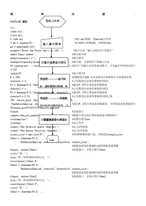
程序流图:MATLAB 源码: clc;clear all;close all;% load mri %载入mri 数据,是matlab 自带库% ph = squeeze(D); %压缩载入的数据D ,并赋值给ph ph = phantom3d(128);prompt={'Enter the Piece num(1 to 128):'}; %提示信息“输入1到27的片的数字”name='Input number'; %弹出框名称defaultanswer={'1'}; %默认数字numInput=inputdlg(prompt,name,1,defaultanswer) %弹出框,并得到用户的输入信息 P= squeeze(ph(:,:,str2num(cell2mat(numInput))));%将用户的输入信息转换成数字,并从ph 中得到相应的片信息Pimshow(P) %展示图片PD = 250; %将D 赋值为250,是从扇束顶点到旋转中心的像素距离。
dsensor1 = 2; %正实数指定扇束传感器的间距2F1 = fanbeam(P,D,'FanSensorSpacing',dsensor1); %通过P ,D 等计算扇束的数据值 dsensor2 = 1; %正实数指定扇束传感器的间距1F2 = fanbeam(P,D,'FanSensorSpacing',dsensor2); %通过P ,D 等计算扇束的数据值dsensor3 = 0.25 %正实数指定扇束传感器的间距0.25 [F3, sensor_pos3, fan_rot_angles3] = fanbeam(P,D,...'FanSensorSpacing',dsensor3); %通过P ,D 等计算扇束的数据值,并得到扇束传感器的位置sensor_pos3和旋转角度fan_rot_angles3figure, %创建窗口imagesc(fan_rot_angles3, sensor_pos3, F3) %根据计算出的位置和角度展示F3的图片colormap(hot); %设置色图为hot colorbar; %显示色栏xlabel('Fan Rotation Angle (degrees)') %定义x 坐标轴ylabel('Fan Sensor Position (degrees)') %定义y 坐标轴output_size = max(size(P)); %得到P 维数的最大值,并赋值给output_size Ifan1 = ifanbeam(F1,D, ... 'FanSensorSpacing',dsensor1,'OutputSize',output_size);%根据扇束投影数据F1及D 等数据重建图像figure, imshow(Ifan1) %创建窗口,并展示图片Ifan1title('图一');disp('图一和原图的性噪比为:');result=psnr1(Ifan1,P);Ifan2 = ifanbeam(F2,D, ...'FanSensorSpacing',dsensor2,'OutputSize',output_size);%根据扇束投影数据F2及D 等数据重建图像figure, imshow(Ifan2) %创建窗口,并展示图片Ifan2disp('图二和原图的性噪比为:');result=psnr1(Ifan2,P);title('图二');Ifan3 = ifanbeam(F3,D, ...生成128的输入图片数字对图片信息进行预处用函数fanbeam 进行映射,得到扇束的数据,并用函数ifanbeam 根据扇束投影数据重建图像,并计算重建图像和原图的结束'FanSensorSpacing',dsensor3,'OutputSize',output_size);%根据扇束投影数据F3及D等数据重建图像figure, imshow(Ifan3) %创建窗口,并展示图片Ifan3title('图三');disp('图三和原图的性噪比为:');result=psnr1(Ifan3,P);function [p,ellipse]=phantom3d(varargin)%PHANTOM3D Three-dimensional analogue of MATLAB Shepp-Logan phantom% P = PHANTOM3D(DEF,N) generates a 3D head phantom that can% be used to test 3-D reconstruction algorithms.%% DEF is a string that specifies the type of head phantom to generate.% Valid values are:%% 'Shepp-Logan' A test image used widely by researchers in% tomography% 'Modified Shepp-Logan' (default) A variant of the Shepp-Logan phantom% in which the contrast is improved for better% visual perception.%% N is a scalar that specifies the grid size of P.% If you omit the argument, N defaults to 64.%% P = PHANTOM3D(E,N) generates a user-defined phantom, where each row% of the matrix E specifies an ellipsoid in the image. E has ten columns,% with each column containing a different parameter for the ellipsoids:%% Column 1: A the additive intensity value of the ellipsoid% Column 2: a the length of the x semi-axis of the ellipsoid% Column 3: b the length of the y semi-axis of the ellipsoid% Column 4: c the length of the z semi-axis of the ellipsoid% Column 5: x0 the x-coordinate of the center of the ellipsoid% Column 6: y0 the y-coordinate of the center of the ellipsoid% Column 7: z0 the z-coordinate of the center of the ellipsoid% Column 8: phi phi Euler angle (in degrees) (rotation about z-axis)% Column 9: theta theta Euler angle (in degrees) (rotation about x-axis) % Column 10: psi psi Euler angle (in degrees) (rotation about z-axis)%% For purposes of generating the phantom, the domains for the x-, y-, and % z-axes span [-1,1]. Columns 2 through 7 must be specified in terms% of this range.%% [P,E] = PHANTOM3D(...) returns the matrix E used to generate the phantom. %% Class Support% -------------% All inputs must be of class double. All outputs are of class double.%% Remarks% -------% For any given voxel in the output image, the voxel's value is equal to the% sum of the additive intensity values of all ellipsoids that the voxel is a% part of. If a voxel is not part of any ellipsoid, its value is 0.%% The additive intensity value A for an ellipsoid can be positive or negative;% if it is negative, the ellipsoid will be darker than the surrounding pixels.% Note that, depending on the values of A, some voxels may have values outside % the range [0,1].%% Example% -------% ph = phantom3d(128);% figure, imshow(squeeze(ph(64,:,:)))%% Copyright 2005 Matthias Christian Schabel (matthias @ stanfordalumni . org) % University of Utah Department of Radiology% Utah Center for Advanced Imaging Research% 729 Arapeen Drive% Salt Lake City, UT 84108-1218%% This code is released under the Gnu Public License (GPL). For more information, % see : /copyleft/gpl.html%% Portions of this code are based on phantom.m, copyrighted by the Mathworks %[ellipse,n] = parse_inputs(varargin{:});p = zeros([n n n]);rng = ( (0:n-1)-(n-1)/2 ) / ((n-1)/2);[x,y,z] = meshgrid(rng,rng,rng);coord = [flatten(x); flatten(y); flatten(z)];p = flatten(p);for k = 1:size(ellipse,1)A = ellipse(k,1); % Amplitude change for this ellipsoidasq = ellipse(k,2)^2; % a^2bsq = ellipse(k,3)^2; % b^2csq = ellipse(k,4)^2; % c^2x0 = ellipse(k,5); % x offsety0 = ellipse(k,6); % y offsetz0 = ellipse(k,7); % z offsetphi = ellipse(k,8)*pi/180; % first Euler angle in radianstheta = ellipse(k,9)*pi/180; % second Euler angle in radianspsi = ellipse(k,10)*pi/180; % third Euler angle in radianscphi = cos(phi);sphi = sin(phi);ctheta = cos(theta);stheta = sin(theta);cpsi = cos(psi);spsi = sin(psi);% Euler rotation matrixalpha = [cpsi*cphi-ctheta*sphi*spsi cpsi*sphi+ctheta*cphi*spsi spsi*stheta;-spsi*cphi-ctheta*sphi*cpsi -spsi*sphi+ctheta*cphi*cpsi cpsi*stheta;stheta*sphi -stheta*cphi ctheta];% rotated ellipsoid coordinatescoordp = alpha*coord;idx = find((coordp(1,:)-x0).^2./asq + (coordp(2,:)-y0).^2./bsq + (coordp(3,:)-z0).^2./csq <= 1);p(idx) = p(idx) + A;endp = reshape(p,[n n n]);return;function out = flatten(in)out = reshape(in,[1 prod(size(in))]);return;function [e,n] = parse_inputs(varargin)% e is the m-by-10 array which defines ellipsoids% n is the size of the phantom brain imagen = 128; % The default sizee = [];defaults = {'shepp-logan', 'modified shepp-logan', 'yu-ye-wang'};for i=1:narginif ischar(varargin{i}) % Look for a default phantomdef = lower(varargin{i});idx = strmatch(def, defaults);if isempty(idx)eid = sprintf('Images:%s:unknownPhantom',mfilename);msg = 'Unknown default phantom selected.';error(eid,'%s',msg);endswitch defaults{idx}case 'shepp-logan'e = shepp_logan;case 'modified shepp-logan'e = modified_shepp_logan;case 'yu-ye-wang'e = yu_ye_wang;endelseif numel(varargin{i})==1n = varargin{i}; % a scalar is the image size elseif ndims(varargin{i})==2 && size(varargin{i},2)==10e = varargin{i}; % user specified phantomelseeid = sprintf('Images:%s:invalidInputArgs',mfilename);msg = 'Invalid input arguments.';error(eid,'%s',msg);endend% ellipse is not yet definedif isempty(e)e = modified_shepp_logan;endreturn;%%%%%%%%%%%%%%%%%%%%%%%%%%%%%% Default head phantoms: % %%%%%%%%%%%%%%%%%%%%%%%%%%%%%function e = shepp_logane = modified_shepp_logan;e(:,1) = [1 -.98 -.02 -.02 .01 .01 .01 .01 .01 .01];return;function e = modified_shepp_logan%% This head phantom is the same as the Shepp-Logan except% the intensities are changed to yield higher contrast in% the image. Taken from Toft, 199-200.%% A a b c x0 y0 z0 phi theta psi% -----------------------------------------------------------------e = [ 1 .6900 .920 .810 0 0 0 0 0 0-.8 .6624 .874 .780 0 -.0184 0 0 0 0-.2 .1100 .310 .220 .22 0 0 -18 0 10-.2 .1600 .410 .280 -.22 0 0 18 0 10.1 .2100 .250 .410 0 .35 -.15 0 0 0.1 .0460 .046 .050 0 .1 .25 0 0 0.1 .0460 .046 .050 0 -.1 .25 0 0 0.1 .0460 .023 .050 -.08 -.605 0 0 0 0.1 .0230 .023 .020 0 -.606 0 0 0 0.1 .0230 .046 .020 .06 -.605 0 0 0 0 ];return;function e = yu_ye_wang%% Yu H, Ye Y, Wang G, Katsevich-Type Algorithms for Variable Radius Spiral Cone-Beam CT %% A a b c x0 y0 z0 phi theta psi% -----------------------------------------------------------------e = [ 1 .6900 .920 .900 0 0 0 0 0 0-.8 .6624 .874 .880 0 0 0 0 0 0-.2 .4100 .160 .210 -.22 0 -.25 108 0 0-.2 .3100 .110 .220 .22 0 -.25 72 0 0.2 .2100 .250 .500 0 .35 -.25 0 0 0.2 .0460 .046 .046 0 .1 -.25 0 0 0.1 .0460 .023 .020 -.08 -.65 -.25 0 0 0.1 .0460 .023 .020 .06 -.65 -.25 90 0 0.2 .0560 .040 .100 .06 -.105 .625 90 0 0-.2 .0560 .056 .100 0 .100 .625 0 0 0 ]; return;% func——计算两幅图像的psnr值function result=psnr1(in1,in2)z=mse(in1,in2);result=10*log10(255.^2/z)% plot(result)function z=mse(x,y)if ndims(x)==3x=rgb2gray(x);endif ndims(y)==3y=rgb2gray(y);endx=double(x);y=double(y);[m1,n1]=size(x);[m2,n2]=size(y);m=min(m1,m2);n=min(n1,n2);z=0;for i=1:mfor j=1:nz=z+(x(i,j)-y(i,j)).^2;endendz=z/(m*n);。
CT图像三维重建附源码
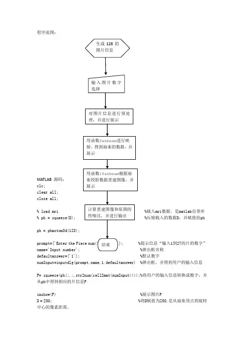
程序流图:MATLAB 源码: clc; clear all;close all;% load mri %载入mri 数据,是matlab 自带库 % ph = squeeze(D); %压缩载入的数据D ,并赋值给phph = phantom3d(128);prompt={'Enter the Piece num(1 to 128):'}; %提示信息“输入1到27的片的数字” name='Input number'; %弹出框名称defaultanswer={'1'}; %默认数字numInput=inputdlg(prompt,name,1,defaultanswer) %弹出框,并得到用户的输入信息P= squeeze(ph(:,:,str2num(cell2mat(numInput))));%将用户的输入信息转换成数字,并从ph 中得到相应的片信息Pimshow(P) %展示图片PD = 250; %将D 赋值为250,是从扇束顶点到旋转中心的像素距离。
生成128的图片信息 输入图片数字选择 对图片信息进行预处理,并进行展示 用函数fanbeam 进行映射,得到扇束的数据,并展示 用函数ifanbeam 根据扇束投影数据重建图像,并展示计算重建图像和原图的性噪比,并进行输出 结束dsensor1 = 2; %正实数指定扇束传感器的间距2F1 = fanbeam(P,D,'FanSensorSpacing',dsensor1); %通过P,D等计算扇束的数据值dsensor2 = 1; %正实数指定扇束传感器的间距1F2 = fanbeam(P,D,'FanSensorSpacing',dsensor2); %通过P,D等计算扇束的数据值dsensor3 = 0.25 %正实数指定扇束传感器的间距0.25 [F3, sensor_pos3, fan_rot_angles3] = fanbeam(P,D,...'FanSensorSpacing',dsensor3); %通过P,D等计算扇束的数据值,并得到扇束传感器的位置sensor_pos3和旋转角度fan_rot_angles3figure, %创建窗口imagesc(fan_rot_angles3, sensor_pos3, F3) %根据计算出的位置和角度展示F3的图片colormap(hot); %设置色图为hotcolorbar; %显示色栏xlabel('Fan Rotation Angle (degrees)') %定义x坐标轴ylabel('Fan Sensor Position (degrees)') %定义y坐标轴output_size = max(size(P)); %得到P维数的最大值,并赋值给output_sizeIfan1 = ifanbeam(F1,D, ...'FanSensorSpacing',dsensor1,'OutputSize',output_size);%根据扇束投影数据F1及D等数据重建图像figure, imshow(Ifan1) %创建窗口,并展示图片Ifan1title('图一');disp('图一和原图的性噪比为:');result=psnr1(Ifan1,P);Ifan2 = ifanbeam(F2,D, ...'FanSensorSpacing',dsensor2,'OutputSize',output_size);%根据扇束投影数据F2及D等数据重建图像figure, imshow(Ifan2) %创建窗口,并展示图片Ifan2disp('图二和原图的性噪比为:');result=psnr1(Ifan2,P);title('图二');Ifan3 = ifanbeam(F3,D, ...'FanSensorSpacing',dsensor3,'OutputSize',output_size);%根据扇束投影数据F3及D等数据重建图像figure, imshow(Ifan3) %创建窗口,并展示图片Ifan3title('图三');disp('图三和原图的性噪比为:');result=psnr1(Ifan3,P);function [p,ellipse]=phantom3d(varargin)%PHANTOM3D Three-dimensional analogue of MATLAB Shepp-Logan phantom% P = PHANTOM3D(DEF,N) generates a 3D head phantom that can% be used to test 3-D reconstruction algorithms.%% DEF is a string that specifies the type of head phantom to generate.% Valid values are:%% 'Shepp-Logan' A test image used widely by researchers in% tomography% 'Modified Shepp-Logan' (default) A variant of the Shepp-Logan phantom % in which the contrast is improved for better % visual perception.%% N is a scalar that specifies the grid size of P.% If you omit the argument, N defaults to 64.%% P = PHANTOM3D(E,N) generates a user-defined phantom, where each row% of the matrix E specifies an ellipsoid in the image. E has ten columns,% with each column containing a different parameter for the ellipsoids:%% Column 1: A the additive intensity value of the ellipsoid% Column 2: a the length of the x semi-axis of the ellipsoid% Column 3: b the length of the y semi-axis of the ellipsoid% Column 4: c the length of the z semi-axis of the ellipsoid% Column 5: x0 the x-coordinate of the center of the ellipsoid% Column 6: y0 the y-coordinate of the center of the ellipsoid% Column 7: z0 the z-coordinate of the center of the ellipsoid% Column 8: phi phi Euler angle (in degrees) (rotation about z-axis)% Column 9: theta theta Euler angle (in degrees) (rotation about x-axis)% Column 10: psi psi Euler angle (in degrees) (rotation about z-axis)%% For purposes of generating the phantom, the domains for the x-, y-, and% z-axes span [-1,1]. Columns 2 through 7 must be specified in terms% of this range.%% [P,E] = PHANTOM3D(...) returns the matrix E used to generate the phantom.%% Class Support% -------------% All inputs must be of class double. All outputs are of class double.%% Remarks% -------% For any given voxel in the output image, the voxel's value is equal to the% sum of the additive intensity values of all ellipsoids that the voxel is a% part of. If a voxel is not part of any ellipsoid, its value is 0.%% The additive intensity value A for an ellipsoid can be positive or negative;% if it is negative, the ellipsoid will be darker than the surrounding pixels.% Note that, depending on the values of A, some voxels may have values outside % the range [0,1].%% Example% -------% ph = phantom3d(128);% figure, imshow(squeeze(ph(64,:,:)))%% Copyright 2005 Matthias Christian Schabel (matthias @ stanfordalumni . org) % University of Utah Department of Radiology% Utah Center for Advanced Imaging Research% 729 Arapeen Drive% Salt Lake City, UT 84108-1218%% This code is released under the Gnu Public License (GPL). For more information, % see : /copyleft/gpl.html%% Portions of this code are based on phantom.m, copyrighted by the Mathworks %[ellipse,n] = parse_inputs(varargin{:});p = zeros([n n n]);rng = ( (0:n-1)-(n-1)/2 ) / ((n-1)/2);[x,y,z] = meshgrid(rng,rng,rng);coord = [flatten(x); flatten(y); flatten(z)];p = flatten(p);for k = 1:size(ellipse,1)A = ellipse(k,1); % Amplitude change for this ellipsoidasq = ellipse(k,2)^2; % a^2bsq = ellipse(k,3)^2; % b^2csq = ellipse(k,4)^2; % c^2x0 = ellipse(k,5); % x offsety0 = ellipse(k,6); % y offsetz0 = ellipse(k,7); % z offsetphi = ellipse(k,8)*pi/180; % first Euler angle in radianstheta = ellipse(k,9)*pi/180; % second Euler angle in radianspsi = ellipse(k,10)*pi/180; % third Euler angle in radianscphi = cos(phi);sphi = sin(phi);ctheta = cos(theta);stheta = sin(theta);cpsi = cos(psi);spsi = sin(psi);% Euler rotation matrixalpha = [cpsi*cphi-ctheta*sphi*spsi cpsi*sphi+ctheta*cphi*spsi spsi*stheta;-spsi*cphi-ctheta*sphi*cpsi -spsi*sphi+ctheta*cphi*cpsi cpsi*stheta;stheta*sphi -stheta*cphi ctheta];% rotated ellipsoid coordinatescoordp = alpha*coord;idx = find((coordp(1,:)-x0).^2./asq + (coordp(2,:)-y0).^2./bsq + (coordp(3,:)-z0).^2./csq <= 1);p(idx) = p(idx) + A;endp = reshape(p,[n n n]);return;function out = flatten(in)out = reshape(in,[1 prod(size(in))]);return;function [e,n] = parse_inputs(varargin)% e is the m-by-10 array which defines ellipsoids% n is the size of the phantom brain imagen = 128; % The default sizee = [];defaults = {'shepp-logan', 'modified shepp-logan', 'yu-ye-wang'};for i=1:narginif ischar(varargin{i}) % Look for a default phantom def = lower(varargin{i});idx = strmatch(def, defaults);if isempty(idx)eid = sprintf('Images:%s:unknownPhantom',mfilename);msg = 'Unknown default phantom selected.';error(eid,'%s',msg);endswitch defaults{idx}case 'shepp-logan'e = shepp_logan;case 'modified shepp-logan'e = modified_shepp_logan;case 'yu-ye-wang'e = yu_ye_wang;endelseif numel(varargin{i})==1n = varargin{i}; % a scalar is the image size elseif ndims(varargin{i})==2 && size(varargin{i},2)==10e = varargin{i}; % user specified phantomelseeid = sprintf('Images:%s:invalidInputArgs',mfilename);msg = 'Invalid input arguments.';error(eid,'%s',msg);endend% ellipse is not yet definedif isempty(e)e = modified_shepp_logan;endreturn;%%%%%%%%%%%%%%%%%%%%%%%%%%%%%% Default head phantoms: % %%%%%%%%%%%%%%%%%%%%%%%%%%%%%function e = shepp_logane = modified_shepp_logan;e(:,1) = [1 -.98 -.02 -.02 .01 .01 .01 .01 .01 .01];return;function e = modified_shepp_logan%% This head phantom is the same as the Shepp-Logan except% the intensities are changed to yield higher contrast in% the image. Taken from Toft, 199-200.%% A a b c x0 y0 z0 phi theta psi% -----------------------------------------------------------------e = [ 1 .6900 .920 .810 0 0 0 0 0 0-.8 .6624 .874 .780 0 -.0184 0 0 0 0-.2 .1100 .310 .220 .22 0 0 -18 0 10-.2 .1600 .410 .280 -.22 0 0 18 0 10.1 .2100 .250 .410 0 .35 -.15 0 0 0.1 .0460 .046 .050 0 .1 .25 0 0 0.1 .0460 .046 .050 0 -.1 .25 0 0 0.1 .0460 .023 .050 -.08 -.605 0 0 0 0.1 .0230 .023 .020 0 -.606 0 0 0 0.1 .0230 .046 .020 .06 -.605 0 0 0 0 ]; return;function e = yu_ye_wang%% Yu H, Ye Y, Wang G, Katsevich-Type Algorithms for Variable Radius Spiral Cone-Beam CT%% A a b c x0 y0 z0 phi theta psi% -----------------------------------------------------------------e = [ 1 .6900 .920 .900 0 0 0 0 0 0-.8 .6624 .874 .880 0 0 0 0 0 0-.2 .4100 .160 .210 -.22 0 -.25 108 0 0-.2 .3100 .110 .220 .22 0 -.25 72 0 0.2 .2100 .250 .500 0 .35 -.25 0 0 0.2 .0460 .046 .046 0 .1 -.25 0 0 0.1 .0460 .023 .020 -.08 -.65 -.25 0 0 0.1 .0460 .023 .020 .06 -.65 -.25 90 0 0.2 .0560 .040 .100 .06 -.105 .625 90 0 0-.2 .0560 .056 .100 0 .100 .625 0 0 0 ];return;% func——计算两幅图像的psnr值function result=psnr1(in1,in2)z=mse(in1,in2);result=10*log10(255.^2/z)% plot(result)function z=mse(x,y)if ndims(x)==3x=rgb2gray(x);endif ndims(y)==3y=rgb2gray(y);endx=double(x);y=double(y);[m1,n1]=size(x);[m2,n2]=size(y);m=min(m1,m2);n=min(n1,n2);z=0;for i=1:mfor j=1:nz=z+(x(i,j)-y(i,j)).^2;endendz=z/(m*n);。
利用Matlab实现原木CT断层图像的三维重建
利用Matlab实现原木CT断层图像的三维重建
张汝楠;孙丽萍
【期刊名称】《木材加工机械》
【年(卷),期】2008(19)4
【摘要】运用MATLAB7.0软件中的图象处理工具箱实现了原木CT断层图像的三维表面重建及体重建(构),原理简单,编程方便,重建速度快,显示效果良好。
【总页数】4页(P24-26)
【关键词】MATLAB;CT图像;表面重建;体重建(构)
【作者】张汝楠;孙丽萍
【作者单位】东北林业大学
【正文语种】中文
【中图分类】S781.1;TP391.41
【相关文献】
1.岩石CT断层序列图像裂纹三维重建的实现 [J], 张飞;姜军周;陈世江
2.MATLAB编程实现连续断层工业CT图像的三维重建 [J], 张爱东;李炬;孙灵霞
3.工业CT断层序列图像三维重建的实现 [J], 赵俊红;瞿中
4.医学CT断层图像三维重建的Matlab实现方法 [J], 穆伟斌;张淑丽
5.利用MATLAB实现CT断层图像的三维重建 [J], 曾筝; 董芳华; 陈晓; 周宏; 周建中
因版权原因,仅展示原文概要,查看原文内容请购买。
基于MATLAB的CT图像三维重建的研究与实现
基于MATLAB的CT图像三维重建的研究与实现张振东1,哈力旦·A2(新疆大学电气工程学院,新疆乌鲁木齐830047)摘要:介绍了利用MATLAB软件对CT切片图像进行三维重建的方法与程序实现。
分别对体绘制法、面绘制法实现的三维重建进行了研究与讨论。
利用MATLAB软件制作GUI界面,实现对肺部CT图像的三维重建以及切分操作。
关键词:体绘制;面绘制;三维重建;GUI界面0 引言CT(Computed Tomography)技术是指利用计算机技术对被测物体断层扫描图像进行重建获得三维断层图像的扫描方式。
自从CT被发明后,CT已经变成一个医学影像重要的工具,虽然价格昂贵,医用X-CT至今依然是诊断多种疾病的黄金准则。
利用X射线进行人体病灶部位的断层扫描,可以得到相应的CT切片图像。
医生可以通过对连续多张CT切片图像的观察,来确定有无病变。
应用三维重建技术可以将连续的二维CT切片图像合成三维可视化图像,便于观察研究。
医学图像的三维建在判断病情、手术设计、医患沟通和医学教学等方面具有很高的研究价值。
CT图像通常是以DICOM格式存储,实验中通常需要转换格式。
本文分别研究讨论了利用MATLAB软件实现对JPG格式的CT切片三维重建的两种常用方法,并制作GUI界面实现切分操作。
1.MATLAB软件在生物切片图像三维重建中的应用MATLAB7.O提供了20类图像处理函数,涵盖了图像处理包括近期研究成果在内的几乎所有的技术方法,是学习和研究图像处理的人员难得的宝贵资料和加工工具箱。
Matlab软件环境提供了各种矩阵运算、操作和图象显现工具。
它已经在生物医学工程,图象处理,统计分析等领域得到了广泛的应用。
在三维重建方面,使用的数据量相对较大,同时涉及到大量的矩阵、光线、色彩、阴影和观察视角的计算,对于非计算机专业研究人员来讲,难度很大。
利用MATLAB 软件中的图像处理函数、工具箱操作,可以大大简化研究。
MATLAB编程实现连续断层工业CT图像的三维重建_张爱东
第26卷 第4期核电子学与探测技术V ol.26 N o.42006年 7月Nuclear Electr onics &Detection T echnolo gyJuly 2006M AT LA B 编程实现连续断层工业CT 图像的三维重建张爱东,李 炬,孙灵霞(中国工程物理研究院,四川绵阳621900)摘要:工业CT 图像的三维重建是无损检测领域的重要组成部分。
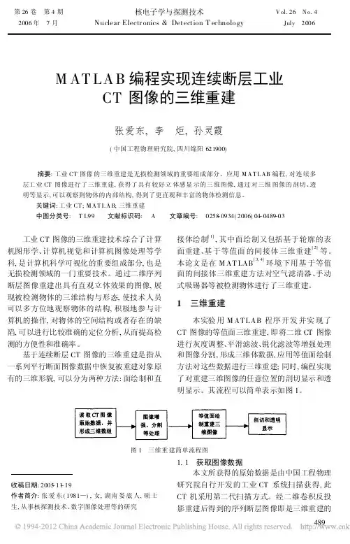
应用M A T L AB 编程,对连续多层工业CT 图像进行了三维重建,获得了具有较好立体感显示的三维图像,通过对三维图像的剖切、透明等显示,可以观察到物体的内部结构,得到了更直观和丰富的物体检测信息。
关键词:工业CT ;M A T L A B;三维重建中图分类号: T L99 文献标识码: A 文章编号: 0258-0934(2006)04-0489-03收稿日期:2005-11-19作者简介:张爱东(1981)),女,湖南娄底人,硕士生,从事核探测技术、数字图像处理等的研究工业CT 图像的三维重建技术综合了计算机图形学、计算机视觉和计算机图像处理等学科,是计算机科学可视化的重要组成部分,也是无损检测领域的一门重要技术。
通过二维序列断层图像重建出具有直观立体效果的图像,展现被检测物体的三维结构与形态,使技术人员可以多方位地观察物体的结构,积极地参与计算机的操作,对物体的空间结构或者存在的缺陷,可以进行比较准确的定位分析,从而提高检测的方便性和准确率。
基于连续断层CT 图像的三维重建是指从一系列平行断面图像数据中恢复被重建对象原有的三维形貌,可以分为两种方法:面绘制和直接体绘制[1],其中面绘制又包括基于轮廓的表面重建、基于等值面的间接体三维重建[2]等。
本论文是在M AT LAB [3,4]环境下用基于等值面的间接体三维重建方法对空气滤清器、手动式吸锡器等被检测物体进行了三维重建。
1 三维重建本实验用M ATLAB 程序开发并实现了CT 图像的等值面三维重建,即将二维CT 图像进行灰度调整、平滑滤波、锐化滤波等增强处理和图像分割,形成三维体数据,应用等值面绘制方法对这些数据进行三维重建;同时,编程实现了对重建三维图像的任意位置的剖切显示和透明显示。
基于MATLAB的脑CT图像三维重建研究
数字诊疗技术与应用Digital Diagnosis and Treatment Technology and Application
数字诊疗技术与应用
Digital Diagnosis and Treatment Technology and Application
的边缘点。
边缘检测算子可以对每个像素的相邻像素值进行检查,并对灰度变化率进行量化,其中也包含对方向的确定,其数学原理是基于方向导数掩模求卷积。
MATLAB 工具箱提供的edge函数可针对sobel算子、canny 算子、zerocross算子、log算子、robert算子和prewitt算子实现检测边
图2 Edge函数不同算子边缘检测效果图
通过比较,本文采用了当下应用广泛的canny算子。
该方法与其他边缘检测方法的主要区别在于,它对强边界和弱边界的检测是通过两个不同的阈值来实现,并且只在二者相连时才进行显示。
所以该方法可在降低噪声影响的同时提高找到真实弱边界的可能。
4.2 关于三维真实感图像显示三维重建完成之后要进行不同角度的显示,同时为了提高显示的效果增加可视性,需要对不需要显示的面进行消隐
图3 Flat模型图
图4 Phong模型图
图5 Gouraud模型图
5 结论
本文介绍了运用MATLAB2007
图1 脑CT图像三维重建效果图Digital Diagnosis and Treatment Technology and Application
数字诊疗技术与应用
《中国数字医学》2015年第10卷第2期。
基于MATLAB超声相控矩阵C扫图片的三维重建
基于MATLAB超声相控矩阵C扫图片的三维重建摘要:超声相控矩阵C扫图像是无损检测的重要组成部分。
应用matlab编程,对超声相控矩阵C扫图像进行三维重建,可以更直观地看到被测样件剖面,截面的缺陷状况,并定位具体缺陷坐标,不但丰富了被测样件的物体检测信息并使其面向观测者更为直观。
Abstract: Ultrasound phased matrix C-scan images are an important part of nondestructive testing. Using MATLAB programming, theultrasonic phased matrix C-scan image is reconstructed in three dimensions, which can more intuitively see the defect status of the section and section of the sample under test, and locate the specific defect coordinates, which not only enriches the object detection information of the sample and makes it more intuitive for the observer.0.引言三维重建作为计算机视觉领域的基础性任务,受到了广泛关注。
而超声相控矩阵技术在无损检测领域于近几年进展迅速。
目前在无损检测领域中,工程师多以单超声相控矩阵b扫或单超声相控c扫对样件进行缺陷分析。
由于单一b,c扫图含有的缺陷信息较少,对样件缺陷的分析效率偏低,又由于单一c扫图所包含的数据量大于单一b扫图像,故本项目选用被测样件的C扫图片进行三维重建。
在程序选择方面,考虑到三维重建需要软件有较好的图像处理能力,故选择matlab为本项目的开发程序。
旧题新作——基于MATLAB的切片三维重建
旧题新作——基于MATLAB的切片三维重建三维重建是计算机图形学和医学图像处理领域的一个重要主题,它使用二维切片图像数据来重建出三维物体模型,对医学诊断、工程设计等领域具有重要意义。
本文基于MATLAB软件,以切片图像数据为输入,利用三维重建算法实现了一个简单的三维重建系统,并对其进行了详细的分析和评测。
2. 数据准备三维重建的输入通常是一组二维切片图像数据,这些数据可以是CT(computed tomography)扫描、MRI(magnetic resonance imaging)扫描等医学影像,也可以是工程设计中的数字化模型的切片数据。
在本文中,我们将使用一个开放的医学影像数据集作为示例数据,以展示三维重建系统的实现过程。
3. 切片图像预处理在进行三维重建之前,我们首先需要对输入的二维切片图像数据进行预处理。
预处理的步骤包括图像格式转换、灰度值标定、噪声去除等。
在MATLAB中,我们可以利用Image Processing Toolbox中的函数来实现这些步骤,例如imread、im2double、imfilter等。
4. 三维重建算法在图像预处理完成后,我们可以开始进行三维重建算法的实现。
三维重建的核心思想是将多个二维切片图像数据拼接起来,然后根据其空间位置关系来还原出三维物体的表面模型。
常见的三维重建算法包括体素化方法、曲面重建方法等。
在本文中,我们将以Marching Cubes算法为例,展示其在MATLAB中的实现过程。
5. 算法实现在MATLAB中实现Marching Cubes算法,需要用到一些基本的图像处理和三维可视化函数。
我们需要将预处理后的二维切片图像数据转换为三维体素数据,这可以通过MATLAB 中的voxeldata函数来实现。
然后,我们需要编写Marching Cubes算法的实现代码,以根据体素数据来还原三维物体的表面模型。
我们可以利用MATLAB中的三维可视化函数,如patch和trisurf,来将还原出的三维表面模型进行可视化展示。
旧题新作——基于MATLAB的切片三维重建
旧题新作——基于MATLAB的切片三维重建切片三维重建可以被描述为一种通过利用二维横截面(切片)图像重新构建三维物体的技术。
这种技术广泛应用于医学影像、工程领域等多个领域。
本文将探讨如何使用MATLAB来进行简单的切片三维重建。
在开始之前,需要了解MATLAB的一些基本概念。
MATLAB是一种数学软件,常用于数学计算、数据分析和可视化,同时也有成熟的图像处理工具箱。
本文所涉及的代码和操作都可以在MATLAB中进行。
首先,需要准备三个不同方向的二维切片图像。
这些图像可以通过CT扫描、MRI等获得,并且需要通过DICOM格式进行导入。
在MATLAB中导入DICOM格式图像的方法如下:```A = dicomread('file.dcm');```其中,file.dcm是DICOM图像文件的名称。
然后,可以将三个不同方向的二维图像组合成一个三维矩阵。
如下所示:```V = cat(4, A1, A2, A3);```其中,A1、A2和A3分别是三个不同方向的二维图像,V为三维矩阵。
在创建完三维矩阵之后,可以使用isosurface函数进行三维表面绘制。
isosurface 函数的使用方法如下:其中,threshold是一个阈值,用于控制三维表面的显示,fv为三维表面上的三角形顶点。
接着,可以使用patch函数将三维表面绘制出来。
具体操作方法如下:如此一来,三维表面就可以显示出来了。
最后,可以使用光源来改善三维显示效果。
MATLAB提供了light函数,可以轻松设置光源。
使用方法如下:```light('Position', [x y z]);```其中,x、y和z是光源的坐标位置。
现在,就可以使用以上几步来实现一个简单的切片三维重建了。
代码如下:```% 导入DICOM格式图像A1 = dicomread('file1.dcm');A2 = dicomread('file2.dcm');A3 = dicomread('file3.dcm');% 使用patch函数将三维表面绘制出来p = patch(fv);% 设置坐标轴axis equal;xlabel('X');ylabel('Y');zlabel('Z');```以上代码将三个不同方向的二维图像组合成一个三维数据矩阵,使用isosurface函数得到三维表面,然后使用patch函数将其绘制出来,并设置光源和坐标轴。
- 1、下载文档前请自行甄别文档内容的完整性,平台不提供额外的编辑、内容补充、找答案等附加服务。
- 2、"仅部分预览"的文档,不可在线预览部分如存在完整性等问题,可反馈申请退款(可完整预览的文档不适用该条件!)。
- 3、如文档侵犯您的权益,请联系客服反馈,我们会尽快为您处理(人工客服工作时间:9:00-18:30)。
基于MATLAB的CT图像三维重建的研究与实现
作者:张振东
来源:《电子世界》2013年第03期
【摘要】介绍了利用MATLAB软件对CT切片图像进行三维重建的方法与程序实现。
分别对体绘制法、面绘制法实现的三维重建进行了研究与讨论。
利用MATLAB软件制作GUI界面,实现对肺部CT图像的三维重建以及切分操作。
【关键词】体绘制;面绘制;三维重建;GUI界面
CT(Computed Tomography)技术是指利用计算机技术对被测物体断层扫描图像进行重建获得三维断层图像的扫描方式。
自从CT被发明后,CT已经变成一个医学影像重要的工具,虽然价格昂贵,医用X-CT至今依然是诊断多种疾病的黄金准则。
利用X射线进行人体病灶部位的断层扫描,可以得到相应的CT切片图像。
医生可以通过对连续多张CT切片图像的观察,来确定有无病变。
应用三维重建技术可以将连续的二维CT切片图像合成三维可视化图像,便于观察研究。
医学图像的三维建在判断病情、手术设计、医患沟通和医学教学等方面具有很高的研究价值。
CT图像通常是以DICOM格式存储,实验中通常需要转换格式。
本文分别研究讨论了利用MATLAB软件实现对JPG格式的CT切片三维重建的两种常用方法,并制作GUI界面实现切分操作。
1.MATLAB软件在生物切片图像三维重建中的应用
MATLAB7.O提供了20类图像处理函数,涵盖了图像处理包括近期研究成果在内的几乎所有的技术方法,是学习和研究图像处理的人员难得的宝贵资料和加工工具箱。
Matlab软件环境提供了各种矩阵运算、操作和图象显现工具。
它已经在生物医学工程,图象处理,统计分析等领域得到了广泛的应用。
在三维重建方面,使用的数据量相对较大,同时涉及到大量的矩阵、光线、色彩、阴影和观察视角的计算,对于非计算机专业研究人员来讲,难度很大。
利用MATLAB软件中的图像处理函数、工具箱操作,可以大大简化研究。
2.常用的三维重建方法
2.1 面绘制
面绘制法是指利用几何单元拼接拟合物体表面来描述物体的三维结构,实现三维重建,也被称为间接绘制方法。
面绘制法的基本原理是从三维数据场中提取出物体的表面部分,用一系列连续的三角形或平面多边形片近似地表示物体的表面特征。
这种近似地方式类,似于用正八十面体表示球面。
2.2 体绘制
直接将体素投影到显示平面的方法称为直接绘制方法,也称为体绘制法。
体绘制是直接利用三维数据场的信息,将整个三维数据场投影出来,达到三维的视觉效果。
体绘制法将数据场中的多种物质在一个可视图中显示,揭示它们的相互关系。
面绘制法相对处理数据量小,重建效果信息量小,外观好,计算速度较快,但是内部简单。
体绘制算法认为体数据场中每个体素都有一定的属性(透明度和光亮度),而且通过计算所有体素对光线的作用即可得到二维投影图像,因此,体绘制可以利用模糊分割的结果,甚至可以不进行分割即可直接进行体绘制。
这样做的好处在于有利于保留了三维医学图像中的细节信息。
因此体绘制算法在对医学图像的重讲具有更好的效果。
3.肺部CT图像的三维重建GUI界面的制作
GUI是Graphical User Interface的简称,即图形用户界面。
MATLAB软件中,提供了制作GUI界面的模块。
利用GUI界面操作运行程序,更为方便直观。
下面介绍GUI界面在肺部CT 图像重建中的应用设计方法。
本实验一共使用连续肺部CT切片20张(图1),利用体绘制方法实现三维重建与部分重建。
GUI界面实现了切分位置的设定以及三个视角的切换功能。
(1)界面设计
利用MATLAB软件设计GUI操作界面,添加“查看原图片”按钮,用于显示原始图片:添加网格效果,便于切分位置的设定。
利用滚动条,可以动态的设置三维切分的参数,可以有针对性的对感兴趣部位进行部分重建观察,来实现切分效果。
“视角选择”中,设置了三个单选按钮,用来调整三维观察的视角。
参数设定完成,点击“三维切分”按钮,实现三维效果。
图像显示于界面右侧。
“清空”按钮用于清除结果,进行下一次操作。
4.结束语
本文主要介绍了常用的两种三维重建方法,认为体绘制方法更适用于医学图像的重建。
此外,重点介绍了利用在MATLAB环境下利用GUI界面实现肺部CT切片体绘制重建界面操作的程序实现方法,该实验实现了三维视角的切换和部分重建位置的设定操作。
三维重建技术在医学领域应用广泛,对它的研究具有重要意义。
参考文献
[1]冈萨雷斯.数字图像处[M].北京:电子工业出版社,2007.
[2]张威,隋天中,赵卫.CT图像表面重建技术中的边缘轮廓提取方法[J].机械科学与技术,2002,21(s1):91-97.
[3]高艳,唐晓英,张军莉,等.基于物体空间序法的cT图像三维重建算法的研究[J].北京生物医学工程,2003,22(3):180-l83.
[4]王成波,陈伟,谢兵,等.DICOM图像与BMP图像的转换研究[J].医疗卫生装备.2004(1):13-17.
[5]穆伟斌,张淑丽.医学CT断层图像三维重建的Matlab实现方法[J].齐齐哈尔大学学报,2009,25(1):33-35.。