ANSYS workbench 裂纹分析
ANSYSworkbench裂纹分析
基于ANSYS Workbench的表面裂纹计算By Yan Fei本教程使用ANSYS Workbench17.0 进行试件表面裂纹的分析,求应力强度因子。
需要提前说明的是,本案例没有工程背景,仅为说明裂纹相的计算方法,因此参数取值比较随意,大量设置都采用了默认值。
1.背景知识传统的强度设计思想把材料视为无缺陷的均匀连续体,而实际工程构件中存在多种缺陷,断裂力学是从20实际50年代末期发展起来的一门弥补了传统强度设计思想严重不足的新的学科,是专门研究含缺陷或裂纹的物体在外界条件作用下构件的强度、裂纹扩展趋势以及疲劳寿命的科学。
断裂力学是从构件内部具有初始缺陷这一实际情况出发,研究在外部荷载下的裂纹扩展规律,从而提出带裂纹构件的安全设计准则。
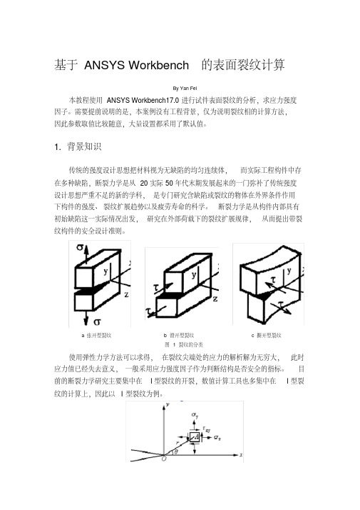
a 张开型裂纹b 滑开型裂纹c 撕开型裂纹图 1 裂纹的分类使用弹性力学方法可以求得,在裂纹尖端处的应力的解析解为无穷大,此时应力值已经失去意义,一般采用应力强度因子作为判断结构是否安全的指标。
目前的断裂力学研究主要集中在I型裂纹的开裂,数值计算工具也多集中在I型裂纹的计算上,因此以I型裂纹为例。
图2 裂纹尖端坐标系含有裂纹的无限大平板的I 型裂纹尖端附近的应力为:)(23cos 2sin 223sin 2sin 12cos223sin 2sin 12cos20ⅠⅠⅠr O r K r K r K xyy x +=+=-=其中,K Ⅰ叫Ⅰ型裂纹的应力强度因子。
2.ANSYS Workbench 裂纹分析2.1.分析模型的建立1 建立一个静力分析步,材料使用默认,需要说明的是,现有计算技术下,断裂力学计算一般都采用线弹性材料,考虑到断裂中塑性区一般都不大,线弹性的假设还是可以接受的。
图3 分析步设置2 建立几何模型,本案例使用spaceclaim 建立几何模型。
图4 试件平面图图5 试件立体图3 分网格,必须采用四面体网格。
本文划分单元特征尺寸1mm。
图 6 网格设置图7 分网效果4 划分网格完成以后,首先进行一次静力计算,确保所有设置正确,对ANSYS Workbench比较熟悉的同学可以省略这一步,静力计算时,试件的两个端面一个约束位移,另一个加1000N的力,方向沿试件轴向,使试件受拉。
ANSYS断裂分析
基于ANSYS的断裂参数的计算1 引言断裂事故在重型机械中是比较常见的,我国每年因断裂造成的损失十分巨大。
一方面,由于传统的设计是以完整构件的静强度和疲劳强度为依据,并给以较大的安全系数,但是含裂纹在役设备还是常有断裂事故发生。
另一方面,对于一些关键设备,缺乏对不完整构件剩余强度的估算,让其提前退役,从而造成了不必要的浪费。
因此,有必要对含裂纹构件的断裂参量进行评定,如应力强度因了和J积分。
确定应力强度因了的方法较多,典型的有解析法、边界配位法、有限单元法等。
对于工程上常见的受复杂载荷并包含不规则裂纹的构件,数值模拟分析是解决这些复杂问题的最有效方法。
本文以某一锻件中取出的一维断裂试样为计算模型,介绍了利用有限元软件ANSYS计算应力强度因子。
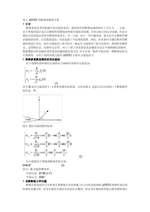
2 断裂参量数值模拟的理论基础对于线弹性材料裂纹尖端的应力场和应变场可以表述为:(1)其中K是应力强度因子,r和θ是极坐标参量,可参见图1,(1)式可以应用到三个断裂模型的任意一种。
图1 裂纹尖端的极坐标系(2)应力强度因子和能量释放率的关系:G=K/E" (3)其中:G为能量释放率。
平面应变:E"=E/(1-v2)平面应力:E=E"3 求解断裂力学问题断裂分析包括应力分析和计算断裂力学的参数。
应力分析是标准的ANSYS线弹性或非线性弹性问题分析。
因为在裂纹尖端存在高的应力梯度,所以包含裂纹的有限元模型要特别注意存在裂纹的区域。
如图2所示,图中给出了二维和三维裂纹的术语和表示方法。
图2 二维和三维裂纹的结构示意图3.1 裂纹尖端区域的建模裂纹尖端的应力和变形场通常具有很高的梯度值。
场值得精确度取决于材料,几何和其他因素。
为了捕获到迅速变化的应力和变形场,在裂纹尖端区域需要网格细化。
对于线弹性问题,裂纹尖端附近的位移场与成正比,其中r是到裂纹尖端的距离。
在裂纹尖端应力和应变是奇异的,并且随1/变化而变化。
为了产生裂纹尖端应力和应变的奇异性,裂纹尖端的划分网格应该具有以下特征:·裂纹面一定要是一致的。
ansys裂纹分析
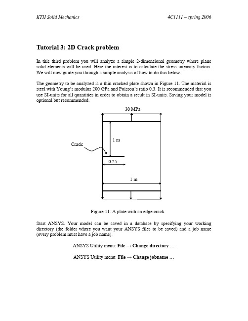
Tutorial 3: 2D Crack problemIn this third problem you will analyze a simple 2-dimensional geometry where plane solid elements will be used. Here the interest is to calculate the stress intensity factors. We will now guide you through a simple analysis of how to do this below.The geometry to be analyzed is a thin cracked plate shown in Figure 11. The material is steel with Young’s modulus 200 GPa and Poisson’s ratio 0.3. It is recommended that you use SI-units for all quantities in order to obtain a result in SI-units. Saving your model is optional but recommended.Figure 11: A plate with an edge crack.Start ANSYS. Your model can be saved in a database by specifying your working directory (the folder where you want your ANSYS files to be saved) and a job name (every problem must have a job name).ANSYS Utility menu: File → Change directory …ANSYS Utility menu: File → Change jobname …GeometryWe will now draw half of (use of symmetry plane) the structure shown in Figure 11 by first defining keypoints and then draw lines between them. Define keypoints at the corners and crack tip, see Figure 12 for the location of the keypoints .ANSYS Main menu: Preprocessor → Modeling → Create → Keypoints → In ActiveCSPress Apply to create the first five keypoints . Press OK to create the last keypoint and close the dialog box.Keypoint x y 1 0 0 2 0.25 0 3 1 04 1 15 0 1 Figure 12: Keypoints coordinates and input dialog box.We will now create lines between the keypoints, see Figure 13 for the order of the lines .ANSYS Main menu: Preprocessor → Modeling → Create → Lines → Lines →Straight LinePress Apply to create the first four lines. Press OK to create the last line and close the dialog box.Line KP1 KP2 1 1 2 2 2 3 3 3 4 4 4 5 5 5 1Figure 13: Lines and keypoints.Tip: You can check your geometry in the graphics display:ANSYS Utility menu: Plot → Keypoints → KeypointsorANSYS Utility menu: Plot → LinesNumbering of lines and keypoints on the graphics display can be turned on and off in the dialog box after selectingANSYS Utility menu: PlotCtrls → Numbering…You are now ready to create an area from the lines:ANSYS Main menu: Preprocessor → Modeling → Create → Areas → Arbitrary →By LinesPick the lines in any order you like. Click OK to create the area.Tip: Remember to save your model every now and then through the analysis.MaterialDefine the material model and the material constants.Element typeThe element type to use is called Plane2. Add this element from the library:ANSYS Main menu: Preprocessor → Element type → Add/Edit/Delete → Add…In the options for the element choose plane stress:ANSYS Main menu: Preprocessor → Element type → Add/Edit/Delete → Options →Element behavior → Plane Stress.MeshIn linear elastic problems, it is known that the displacements near the crack tip (or crack front) vary asr,where r is the distance from the crack tip. The stresses and strains are singular at the crack tip, varying asr1.To resolve the singularity in strain, the crack faces should be coincident, and the elements around the crack tip (or crack front) should be quadratic, with the midside nodes placed at the quarter points. Such elements are called singular elements . Figure 14 shows an example of a 2D singular element.Figure 14: Example of a 2D singular element and element- division around a crack tip.The first row of element around the crack tip should be singular as illustrated above. The KSCON command which assigns element division sizes around a keypoint, is particularly useful in a fracture model. It automatically generates singular elements around the specified keypoint. Other fields on the command allow you to control the radius of the first row of elements, number of elements in the circumferential direction, etc. KSCON is found inANSYS Main menu: Preprocessor → Meshing → Size Cntrls → Concentrat KPs →Create.Select the crack tip keypoint. Choose the element size closest to the crack tip to be 0.001 of the crack length, the radius ratio to 1.5 and number of elements in the circumferential direction to 6. Also, don’t forget to change the midside node position to ¼ pt, see Figure 15.Figure 15: The dialog box appearing in the KSCON command.Before meshing the area a global size limitation on the element size should be set. This is not necessary for the problem to be solved but can improve the condition number of the stiffness matrix.ANSYS Main menu: Preprocessor → Meshing → Size Cntrls → ManualSize →Global → Size…Choose the global size to 0.05 m. Now you are ready to mesh the area with command: ANSYS Main menu: Preprocessor → Meshing → Mesh → Areas → Free.Pick the area and click OK.LoadsAs only half of the geometry is modeled, symmetry boundary condition should be applied on the symmetry plane:ANSYS Main menu: Solution → Define Loads → Apply → Structural →Displacement → Symmetry B.C. → On linesPick line number 2 and click OK. The crack surface is not restricted in its movement in any direction that is no boundary condition should be applied to that line. Of course, if a negative force is applied and the crack surfaces moves towards each other, a contact definition needs to be defined. But here we assume that the crack surfaces moves away from each other.Apply the load on the top line of the model as pressure. The pressure is defined positive in the negative normal direction; therefore a minus sign should be included when defining the pressure. The command is:ANSYS Main menu: Solution → Define Loads → Apply → Structural → Pressure →On Lines,where line number 4 is picked. A new box appears and the pressure can be defied as a constant value, -30e6 Pa. By default is the thickness assumed to be of unit size in Ansys. SolutionThe problem is now defined and ready to be solved:ANSYS Main menu: Solution → Solve → Current LSResultsEnter the postprocessor and read in the results:ANSYS Main menu: General Postproc → Read Results → First SetNow there are several results to study. Plot the deformed and undeformed shapes, this has been described earlier. Also, study the elements solution of the von Mises stress around the crack tip. The stress-level should be quite high at the crack tip since the elasticity theory gives infinity large stresses around a crack tip. The higher resolution of the mesh the higher stress-levels will be obtained.The stress-intensity factors may now be of interest. The KCALC command calculates the mixed-mode stress intensity factors K I, K II, and K III. This command is limited to linear elastic problems with a homogeneous, isotropic material near the crack region. To use KCALC properly, follow these steps in the General Postprocessor:1.Define a local crack-tip or crack-front coordinate system, with X parallel to thecrack face (perpendicular to the crack front in 3-D models) and Y perpendicular to the crack face, as shown in the following Figure 16.Figure 16: Local coordinate system at the crack tip.This coordinate system must be the active model coordinate system and also theresults coordinate system when KCALC is issued.The local coordinate system is defined through:Utility Menu → WorkPlane → Local Coordinate Systems → Create LocalCS → At Specified LocChoose the keypoint at the crack tip and the following dialog box appears. Fill in as below and click OK.Figure 17: Dialog box appearing at the Create Local CS command.You have now set the reference number to 11 for the local coordinate system.To turn the local coordinate system into active, use the following command: Utility Menu → WorkPlane → Change Active CS to → Specified CoordSys…Change to coordinate system number 11 as defined above.To change the results coordinate system, use the following command:ANSYS Main menu: General Postproc → Options for Outp.The command activates a coordinate system for printout or display of element and nodal results. Change the RSYS in the dialog box to local system and link to the created system above by typing in the reference number.2. Define a path along the crack face. The first node on the path should be the crack-tip node. For a half-crack model, two additional nodes are required, both along the crack face, see Figure 18.Tip: If it is hard to see the actual crack tip node, choose to plot the nodes by use of command:Utility Menu → Plot → Nodes.1Figure 18: The nodes to be chosen in the Path definition.ANSYS Main menu: General Postproc → Path Operations → Define Path. 3. Calculate K I, K II, and K III. The KPLAN field on the KCALC command specifieswhether the model is plane-strain or plane stress. Except for the analysis of thin plates, the asymptotic or near-crack-tip behavior of stress is usually thought to be that of plane strain. The KCSYM field specifies whether the model is a half-crack model with symmetry boundary conditions, a half-crack model with antisymmetry boundary conditions, or a full-crack model. In this case you have a symmetric half-crack model.ANSYS Main menu: General Postproc → Nodal Calcs → Stress Int Factr。
ANSYS静力学 裂纹钻孔止裂前后及不同钻孔直径下的应力分析

Ansys 作业:裂纹钻孔止裂前后及不同钻孔直径下的应力分析裂纹钻孔止裂前后及不同钻孔直径下的应力分析目前钢结构广泛应用于桥梁、机械、工业和公共建筑,对其维护的重要性也显得越来越突出。
疲劳裂纹是一种钢结构常见的破坏形式,当发现钢结构构件中萌生了疲劳裂纹时,可以采用钻孔止裂技术,在裂纹尖端钻孔消除裂纹尖端的应力集中,从而延长钢结构构件的疲劳寿命,既确保了安全,又避免了不必要的损失。
而钻孔止裂技术的止裂效果取决于疲劳裂纹在止裂孔边的再生寿命,止裂孔直径的大小将直接影响疲劳裂纹的再生寿命,因此,对构件进行钻孔止裂分析十分重要。
一、创建有限元模型以钢板分析为例: 长100m 宽80m 厚0.002m裂纹区域坐标 (-40,0.01,0) (-40,0.01,0,) (-39.9,0,0)弹性模量泊松比建模时,只建立面,以矩形中心为坐标原点,厚度在中如下设置划分后的单元二、设定载荷并求解左上点、右下点固定段约束上下两边压强三、后处理模型1变形情况:Mises应力云图四、不同钻孔直径下的Mises应力云图1、直径0.002m2、直径0.004m3、直径0.006m4、直径0.008m五、数据分析:/减小,裂纹尖端的应力集中现象的得到改善。
本次模拟试验为验证性试验,实际应用中裂纹尖端钻孔可以降低应力集中现象,但改善情况一般在30%以内,本次模拟实验的到的应力改善情况偏大,应该是划分单元的粗细程度不同引起的。
3、纵向比较不同直径的钻孔可知:应力集中现象的最大的应力值随孔径的增大而减小。
但由实际可知,钻孔并非越大越好,故上述结论在一定范围内是成立的。
Ansys 断裂力学理论
第四章断裂力学文献来源:/document/200707/article796_2.htm4.1 断裂力学的定义在许多结构和零部件中存在的裂纹和缺陷,有时会导致灾难性的后果。
断裂力学在工程领域的应用就是要解决裂纹和缺陷的扩展问题。
断裂力学是研究载荷作用下结构中的裂纹是怎样扩展的,并对有关的裂纹扩展和断裂失效用实验的结果进行预测。
它是通过计算裂纹区域和破坏结构的断裂参数来预测的,如应力强度因子,它能估算裂纹扩展速率。
一般情况下,裂纹的扩展是随着作用在构件上的循环载荷次数而增加的。
如飞机机舱中的裂纹扩展,它与机舱加压及减压有关。
此外,环境条件,如温度、或大范围的辐射都能影响材料的断裂特性。
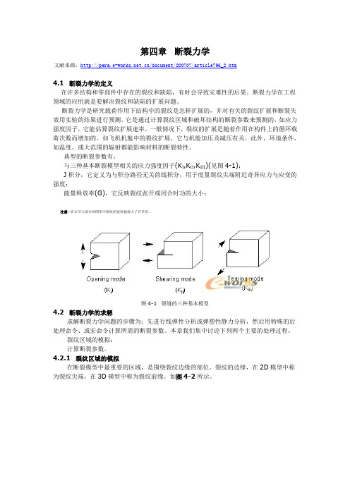
典型的断裂参数有:与三种基本断裂模型相关的应力强度因子(K I,K II,K III)(见图4-1);J积分,它定义为与积分路径无关的线积分,用于度量裂纹尖端附近奇异应力与应变的强度;能量释放率(G),它反映裂纹张开或闭合时功的大小;注意--在本节大部分的图形中裂纹的宽度被放大了许多倍。
图4-1 裂缝的三种基本模型4.2 断裂力学的求解求解断裂力学问题的步骤为:先进行线弹性分析或弹塑性静力分析,然后用特殊的后处理命令、或宏命令计算所需的断裂参数。
本章我们集中讨论下列两个主要的处理过程。
裂纹区域的模拟;计算断裂参数。
4.2.1 裂纹区域的模拟在断裂模型中最重要的区域,是围绕裂纹边缘的部位。
裂纹的边缘,在2D模型中称为裂纹尖端,在3D模型中称为裂纹前缘。
如图4-2所示。
图4-2 裂纹尖端和裂纹前缘在线弹性问题中,在裂纹尖端附近(或裂纹前缘)某点的位移随而变化,γ是裂纹尖端到该点的距离,裂纹尖端处的应力与应变是奇异的,随1/变化。
为选取应变奇异点,相应的裂纹面需与它一致,围绕裂纹顶点的有限元单元应该是二次奇异单元,其中节点放到1/4边处。
图4-3表示2-D和3-D模型的奇异单元。
图4-3 2-D和3-D模型的奇异单元4.2.1.1 2-D断裂模型对2D断裂模型推荐采用PLANE2单元,其为六节点三角形单元。
利用ANSYS进行断裂分析
利用ANSYS进行断裂分析初次试做断裂分析,希望有这方面经验的高手能发表些经验之谈!这个模型由两种材料组成:表面镀层为铝,基底为钢。
目的是对表面镀层的剥离过程进行分析。
目前这个模型是个假想的简化模型,初步目标是实现剥离过程的模拟。
裂纹扩展是通过接触单元生死功能实现的。
基层和镀层由接触单元连接,然后通过断裂判断准则确定要杀死的失效的接触单元。
第一版(没有加断裂判断准则,强行逐个杀死界面接触单元):fini/clear/filn,crack1/PREP7!*ET,1,PLANE182!*KEYOPT,1,1,2KEYOPT,1,3,1KEYOPT,1,4,0KEYOPT,1,6,0KEYOPT,1,10,0!*rect,0,100,0,100rect,0,100,100,110lesi,1,,,10lesi,2,,,10esha,2!*MPTEMP,,,,,,,,MPTEMP,1,0MPDATA,EX,1,,210e3MPDATA,PRXY,1,,0.3MPTEMP,,,,,,,,MPTEMP,1,0MPDATA,EX,2,,70MPDATA,PRXY,2,,0.33amesh,1lesi,5,,,10lesi,6,,,2mat,2amesh,2lsel,s,,,3nsll,s,1cm,c1,nodelsel,s,,,5nsll,s,1cm,t1,nodensel,s,loc,xd,all,uxnsel,s,loc,yd,all,uyd,all,uxmp,mu,3,0/COM, CONTACT PAIR CREATION - START CM,_NODECM,NODECM,_ELEMCM,ELEMCM,_LINECM,LINECM,_AREACM,AREA/GSA V,cwz,gsav,,tempMP,MU,3,0MA T,3R,3REAL,3ET,2,169ET,3,172R,3,,,100,0.1,0,RMORE,,,1.0E20,0.0,1.0,RMORE,0.0,0,1.0,,1.0,0.5RMORE,0,0.5,1.0,0.0,KEYOPT,3,2,0KEYOPT,3,3,0KEYOPT,3,4,0KEYOPT,3,5,0KEYOPT,3,7,0KEYOPT,3,8,0KEYOPT,3,9,0KEYOPT,3,10,0KEYOPT,3,11,0KEYOPT,3,12,5! Generate the target surfaceNSEL,S,,,T1CM,_TARGET,NODETYPE,2ESLN,S,0ESURF,ALLCMSEL,S,_ELEMCM! Generate the contact surfaceNSEL,S,,,C1CM,_CONTACT,NODETYPE,3ESLN,S,0ESURF,ALLALLSELESEL,ALLESEL,S,TYPE,,2ESEL,A,TYPE,,3ESEL,R,REAL,,3/PSYMB,ESYS,1/PNUM,TYPE,1/NUM,1EPLOTESEL,ALLESEL,S,TYPE,,2ESEL,A,TYPE,,3ESEL,R,REAL,,3CMSEL,A,_NODECMCMDEL,_NODECMCMSEL,A,_ELEMCMCMDEL,_ELEMCMCMSEL,S,_LINECMCMDEL,_LINECMCMSEL,S,_AREACMCMDEL,_AREACM/GRES,cwz,gsavCMDEL,_TARGETCMDEL,_CONTACT/COM, CONTACT PAIR CREATION - END lsel,s,,,7nsll,s,1cm,s1,node!Gradient surface loadSFGRAD,PRES,0,X,0,-0.1,sf,all,pres,-0.1nsel,allesel,all!save/solutime,1deltim,1,1,1solve/post1plns,s,1anty,,resttime,1.1ekill,140solve/post1plns,s,1/soluanty,,resttime,1.2ekill,140ekill,139solve/post1plns,s,1/soluanty,,resttime,1.3ekill,140ekill,139ekill,138solve/post1plns,s,1/soluanty,,resttime,1.4ekill,140ekill,139ekill,138ekill,137solve/post1plns,s,1第二版(加了断裂自动判断准则)。
基于ANSYS Workbench的均压环断裂分析

基于ANSYS Workbench的均压环断裂分析王益博;杨乐;孟忠;莫冰;马梁丁;康鹏【摘要】The grading ring is an important part of the high voltage electrical equipment. It is mainly used for balancing the stray capacitance and distributing the voltage evenly. Under a large force of wind load, the HV switch disconnectorgrading ring operating in high winds area is very important for its own design strength and operational reliability. Based on the ANSYS Workbench18. 1finite element analysis software, a fracture problem of the HV switch disconnector-grading ring caused by strong wind force is analyzed. The calculation condition determination, the stress analysis, the model establishment, the stress surface cutting and the simulation calculation are carried out in step. The displacement and stress of the HV switch disconnector-grading ring under wind load are obtained. The results show that the manufacturing quality of the grading ring is the main factor affecting the strength and reliability of the grading ring when the design strength of the grading ring meets the requirements of operation. Some measures to improve the strength and reliability of the HV switch disconnector- grading ring are put forward.%均压环是高压电器设备的重要组成部分, 其主要作用是均衡对地杂散电容, 使电压分布均匀.运行在大风地区的高压隔离开关均压环, 在风载荷的较大作用力下, 其自身的设计强度和运行可靠性至关重要.基于ANSYS Workbench18. 1有限元分析软件, 对由于大风作用力引起的均压环断裂问题进行逐步分析, 通过确定计算条件、进行受力分析、建立模型和仿真计算等, 分析得出该均压环在较大的风载荷作用力下的位移和应力情况.结果表明, 在保证均压环的设计强度满足使用要求的情况下, 均压环的制造质量是影响其强度和运行可靠性的主要因素.给出了提高高压隔离开关均压环强度及运行可靠性的具体措施.【期刊名称】《新技术新工艺》【年(卷),期】2018(000)004【总页数】3页(P67-69)【关键词】高压隔离开关均压环;大风;ANSYS;强度;分析;可靠性【作者】王益博;杨乐;孟忠;莫冰;马梁丁;康鹏【作者单位】西安西电高压开关有限责任公司,陕西西安 710018;西安西电高压开关有限责任公司,陕西西安 710018;西安西电高压开关有限责任公司,陕西西安710018;西安西电高压开关有限责任公司,陕西西安 710018;西安西电高压开关有限责任公司,陕西西安 710018;西安西电高压开关有限责任公司,陕西西安 710018【正文语种】中文【中图分类】TM564.1我国西北部存在诸多强风气候区域,以新疆为例,从其西部的阿拉山口到东部的哈密地区之间就存在八大著名风区,其中,以达坂城至吐鲁番、阿拉山口至七角井最为著名[1]。
混凝土结构的裂缝及其ANSYS分析
混凝土结构的裂缝及其ANSYS分析混凝土结构是建筑工程中常见的结构形式,由于其性能优异,在各种建筑中被广泛使用。
然而,由于混凝土结构的特性,如收缩、膨胀、温度变化、荷载变形等,可能会导致结构出现裂缝。
本文将探讨混凝土结构的裂缝产生原因、裂缝的分类以及使用ANSYS软件进行裂缝分析的方法。
混凝土结构的裂缝产生原因可以从内力和外力两个方面考虑。
内力是由于结构收缩、膨胀和变形引起的,外力则包括温度变化、荷载作用、水膨胀、地震等因素。
裂缝的形成是由于混凝土内部受到拉应力的作用,当拉应力超过混凝土的抗拉强度时,就会形成裂缝。
根据混凝土结构裂缝的性质和产生原因,常见的裂缝可以分为以下几类:1.收缩裂缝:由于混凝土在干燥过程中会发生收缩,造成内部产生拉应力,从而形成的裂缝。
2.膨胀裂缝:由于温度的变化以及聚合材料的膨胀引起的裂缝,也是常见的一种裂缝类别。
3.荷载裂缝:由于承载结构受到外部荷载作用产生的拉应力引起的裂缝。
4.施工裂缝:由于混凝土的收缩和膨胀,以及施工技术不良等因素引起的裂缝。
5.水膨胀裂缝:由于混凝土受到水的侵蚀,引起水膨胀引起的裂缝。
为了对混凝土结构的裂缝进行分析,可以使用ANSYS软件。
ANSYS是一种通用有限元分析软件,可以用于模拟和分析各种复杂的结构问题。
以下是使用ANSYS进行混凝土结构裂缝分析的方法:1.准备模型:首先需要准备一个混凝土结构的三维模型。
可以使用CAD软件绘制模型,然后导入到ANSYS中。
在绘制模型时,需要注意表达混凝土的材料性质、尺寸和边界条件等。
2.定义材料性质:在ANSYS中定义混凝土的材料性质,包括弹性模量、抗拉强度、抗压强度、收缩系数等参数。
这些参数可以根据实际材料的性质进行设定。
3.应用载荷:在模型中应用实际的载荷和边界条件。
载荷可以包括静载荷、动态荷载以及温度载荷等。
需要注意的是,载荷应符合实际工程情况。
4.网格划分:将模型进行网格划分,将结构划分成小的单元。
- 1、下载文档前请自行甄别文档内容的完整性,平台不提供额外的编辑、内容补充、找答案等附加服务。
- 2、"仅部分预览"的文档,不可在线预览部分如存在完整性等问题,可反馈申请退款(可完整预览的文档不适用该条件!)。
- 3、如文档侵犯您的权益,请联系客服反馈,我们会尽快为您处理(人工客服工作时间:9:00-18:30)。
基于ANSYS Workbench的表面裂纹计算
By Yan Fei
本教程使用ANSYS Workbench17.0 进行试件表面裂纹的分析,求应力强度因子。
需要提前说明的是,本案例没有工程背景,仅为说明裂纹相的计算方法,因此参数取值比较随意,大量设置都采用了默认值。
1.背景知识
传统的强度设计思想把材料视为无缺陷的均匀连续体,而实际工程构件中存在多种缺陷,断裂力学是从20实际50年代末期发展起来的一门弥补了传统强度设计思想严重不足的新的学科,是专门研究含缺陷或裂纹的物体在外界条件作用下构件的强度、裂纹扩展趋势以及疲劳寿命的科学。
断裂力学是从构件内部具有初始缺陷这一实际情况出发,研究在外部荷载下的裂纹扩展规律,从而提出带裂纹构件的安全设计准则。
a 张开型裂纹
b 滑开型裂纹
c 撕开型裂纹
图 1 裂纹的分类
使用弹性力学方法可以求得,在裂纹尖端处的应力的解析解为无穷大,此时应力值已经失去意义,一般采用应力强度因子作为判断结构是否安全的指标。
目前的断裂力学研究主要集中在I型裂纹的开裂,数值计算工具也多集中在I型裂纹的计算上,因此以I型裂纹为例。
图2 裂纹尖端坐标系
含有裂纹的无限大平板的I 型裂纹尖端附近的应力为:
)(23cos 2sin 223sin 2sin 12cos 223sin 2sin 12cos 20ⅠⅠⅠr O r K r
K r
K xy y x +⎪⎪⎪⎪⎭⎪⎪⎪⎪⎬⎫=⎪⎭⎫ ⎝⎛+=⎪⎭⎫ ⎝⎛−=θθπτθθθπσθθθπσ
其中,K Ⅰ叫Ⅰ型裂纹的应力强度因子。
2. ANSYS Workbench 裂纹分析
2.1. 分析模型的建立
1 建立一个静力分析步,材料使用默认,需要说明的是,现有计算技术下,断裂力学计算一般都采用线弹性材料,考虑到断裂中塑性区一般都不大,线弹性的假设还是可以接受的。
图3 分析步设置
2 建立几何模型,本案例使用spaceclaim 建立几何模型。
图4 试件平面图
图5 试件立体图
3 分网格,必须采用四面体网格。
本文划分单元特征尺寸1mm。
图 6 网格设置
图7 分网效果
4 划分网格完成以后,首先进行一次静力计算,确保所有设置正确,对ANSYS Workbench比较熟悉的同学可以省略这一步,静力计算时,试件的两个端面一个约束位移,另一个加1000N的力,方向沿试件轴向,使试件受拉。
从图9可以看出,网格、约束、荷载等设置正常。
图8 荷载设置
图9 约束设置
图9 不含裂纹的计算结果
5 在左上角的特征树上model部分点击右键,选择insert—fracture。
引入缺陷特征。
此时特征树上回出现fracture模块,如图10 所示。
然后再coordinate system 上点右键,建立一个用户坐标系,用于指示裂纹的位置,新建立的坐标系原点应该位于半椭圆裂纹中心处,X轴指向材料内部。
其设置如图11所示,结果如图12所示。
图10 包含fracture模块的特征树
图11 新坐标系的设置
图12 新坐标系的位置(红色为1轴,即X轴)
6 在特征树中的fracture上右击,选择insert—semi-ellipical crack。
裂纹参数设置如图所示。
其中比较重要的参数包括裂纹的半长轴长度1mm.半短轴长度
0.5mm,裂纹尖端(再此处为一半椭圆曲线)划分的网格数10,积分围道数5等。
图13 裂纹参数
图14 裂纹效果
7 更新网格,这次分网会比较慢,如果没有设置错,这时候就能看到裂纹处的网格了。
ANSYS这一点比较好,不像ABAQUS需要自己分网。
图15 裂纹处的网格
8 提交计算,因为之前做静力计算的时候荷载什么的都已经施加了,不需要再做处理,跳过那一步的该补荷载的补荷载,该补约束的补约束。
这次侧计算会比静力计算慢一点点。
图16 整体应力(mises应力)
图17 裂纹尖端应力(mises应力)
9 后处理,在特征树上的solution上右击,insert—fracture tool添加后处理工具,然后在模型树上点击fracture tool,选择裂纹(如图18)。
图18 选择裂纹
10 右击fracture—insert—SIFS, fracture—insert—J-integral ,分别添加应力强度因子和J积分。
然后更新结果,皆可以看到应力强度因子和J积分的结果了。
J积分结果如图19和图20。
图19 应力强度因子云图
图20 应力强度因子曲线图。