物理-曲柄滑块机构的运动分析-matlab备课讲稿
曲柄滑块机构的运动精度分析与计算
曲柄滑块机构的运动精度分析与计算宋亮;赵鹏兵【摘要】曲柄滑块机构是一种典型的四连杆机构,尽管设计时理论计算可以达到很高的精度,但是由于构件的制造误差及运动副的配合间隙等因素,会使机构在运动中产生输出误差,有时还会显著超出机构设计的允许误差.依据概率统计的相关理论进行机构设计,即考虑构件制造尺寸的随机误差,以保证机构运动的精度在允许的误差范围内.利用MATLAB进行仿真计算和实例研究,得出了理论设计和精度分析的计算结果.该方法准确、效率高、而且适合其它类型的机构设计,具有较大的工程实际应用价值.%Slider-crank mechanism is a typical four-bar linkage, in spite of the high precision when it' s calculated theoretically. The manufacturing error and kinematic pair clearance of the components will lead to the output error during the motion of the mechanism. Sometimes,it will significantly exceed the tolerance of the design. According to the probability and statistics theory, the mechanism is designed, that' s considering the random error of the component to make sure that the motion accuracy is in the allowed error range. Utilizing MATLAB to simulate and calculate based on case studies. and the theoretical design and accuracy analysis are obtained. This method is accurate and very efficiently, it also can be used in other kind of mechanism design, and it has much more practical value in engineering.【期刊名称】《科学技术与工程》【年(卷),期】2011(011)010【总页数】5页(P2201-2205)【关键词】曲柄滑块机构;运动学;概率设计;等影响法;精度分析【作者】宋亮;赵鹏兵【作者单位】海军装备部,西安,710043;西北工业大学现代设计与集成制造技术教育部重点实验室,西安,710072【正文语种】中文【中图分类】TH112.1曲柄滑块机构是一种单移动副的四连杆机构,如图1和图2所示,分别为对心和偏心曲柄滑块机构。
基于MATLAB曲柄滑块机构的运动学分析
农 机 使 用 与 维 修
2 1 ] p L B曲柄 滑 块 机 构 的 TA 运 动 学 分 析
黑 龙江八一农垦大学工程学院 张欣悦 李连豪 王
摘 要
涛
MA L B运动仿真技术是借助计算机技术和 MA L B软件技 术平 台发展起 来的一种分析机 械运动 参数 TA TA
t r s c mp e t e u e i o lx,h n MATL r g a ln u g s e se o ma i u a e I hi a e ld r—c a k AB p o rm a g a e i a ir t n p l t . n t s p p ra si e rn me h ns a n e a l a ay e tb a s o c a im s a x mp e, n l s d i y me n fMAT LAB Moin S mu a in, r u h isv s lf n . to i l t o Th o g t iua u c to re o e p e s si e — r nk me h nim ̄ moi n p r me e si it r y in tid t x r s ld r— c a c a s to aa tr n a p cu e wa 。 Ke r s:MATL y wo d AB; l e si r—c a k; i e t s a ay i d r n k n ma i ; n l ss c
解答 。
过 曲柄 滑 块 机 构 这 一 理 论 模 型 的普 遍 性 角 度 去 研
究, 当然 这也 是本 文 的不 足之 处 , 而导 致 在解 决 实 从 际 问题 时 的具 体模 拟分 析时 出现偏 差 。
基于matlab的曲柄滑块机构设计与运动分析_陈长秀
变,从第 i+1 个功能块开始逐位交换。
(3)变异运算的改进
由于在每个功能块中,“1”的数目即是该题型试题的数目, 因此在变异过程中应保证整个种群所有功能块中“1”的数目不 变。可执行如下过程,首先,由变异概率决定某位取反;然后,检 查、修正字符串中“1”的数目,保证不发生变化。
(4)用全局最优解替换本次迭代的最差解 为保证好的字符串不至于流失,每次遗传操作前记录本次 迭代的最优解,若该解优于全局最优解则替换全局最优解,否 则全局最优解保持不变。此次遗传操作后,用全局最优解换本 代的最差解。
(上接第 29 页)
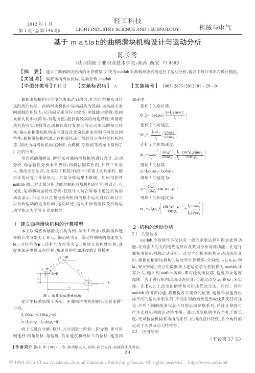
图 1 所示的偏置曲柄滑块机构。设 l1=50mm,l2=100mm, e=20mm,w1=2rad/s,设 φ1 的初始值为 0 , 则 φ1 变化时,杆 2 的角位移、角速度和角加速度以及滑块 3 的位移、速度和加速
>> plot(t,xc,t,vc,t,ac);
度的变化值可计算求得,曲柄转角 φ1 在 0- 360°之间变化时, 在 matlab 的计算窗口输入算式后,滑块 3 的位移、速度和加速
2012 年 1 月 第 1 期(总第 158 期)
轻工科技
LIGHT INDUSTRY SCIENCE AND TECHNOLOGY
机械与电气
基于 m a tla b 的曲柄滑块机构设计与运动分析
陈长秀
(陕西国防工业职业技术学院,陕西 西安 71 0302)
【摘 要】 建立了曲柄滑块机构的计算模型,并使用 matlab 对曲柄滑块机构进行了运动分析,提高了设计效率和设计精度。
图 1 偏置曲柄滑块机构 建立坐标系如图 1 所示,由曲柄滑快机构的矢量封闭图[1] 可得:
φl1 cosφ1+l2 cosφ2=xc
基于MATLAB曲柄滑块机构运动仿真
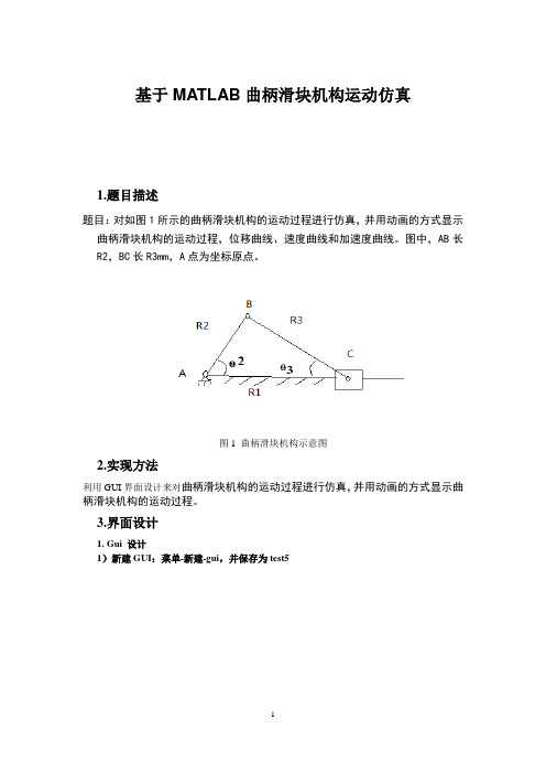
基于MATLAB曲柄滑块机构运动仿真1.题目描述题目:对如图1所示的曲柄滑块机构的运动过程进行仿真,并用动画的方式显示曲柄滑块机构的运动过程,位移曲线、速度曲线和加速度曲线。
图中,AB长R2,BC长R3mm,A点为坐标原点。
图1 曲柄滑块机构示意图2.实现方法利用GUI界面设计来对曲柄滑块机构的运动过程进行仿真,并用动画的方式显示曲柄滑块机构的运动过程。
3.界面设计1. Gui 设计1)新建GUI:菜单-新建-gui,并保存为test52)界面设计:拖拽左侧图标到绘图区,创建GUI界面拖拽左侧图标值绘图区设置如下的按钮最终的仿真界面如图所示3)代码添加:进入代码界面4.代码编程%模型求解a1=str2double(get(handles.edit1,'String'));a2=str2double(get(handles.edit2,'String'));a3=str2double(get(handles.edit3,'String'));a4=str2double(get(handles.edit4,'String'));a5=str2double(get(handles.edit5,'String'));a=a1*((1-cos(a4*a5))+0.25*(a1/a2)*(1-cos(2*a4*a5))); set(handles.edit6,'String',a);a0=(a4*a1)*(sin(a4*a5)+0.5*(a1/a2)*sin(2*a4*a5));set(handles.edit7,'String',a0);a6=(a4*a4*a1)*(cos(a4*a5)+(a1/a2)*cos(a4*a5));set(handles.edit8,'String',a6);%绘制位移、速度、加速度曲线axes(handles.axes3);r1=str2double(get(handles.edit1,'String'));r2=str2double(get(handles.edit2,'String'));omiga1=str2double(get(handles.edit4,'String'));x11=1:720;for i=1:720x1(i)=i*pi/180;%sin(x2(i)=r1/r2*sin(x1(i));x2(i)=asin(-r1/r2*sin(x1(i)));x22(i)=x2(i)*180/pi;r3(i)=r1*cos(x1(i))+r2*cos(x2(i));B=[-r1*omiga1*sin(x1(i));r1*omiga1*cos(x1(i))];A=[r2*sin(x2(i)) 1;-r2*cos(x2(i)) 0];X=inv(A)*B;omiga2(i)=X(1,1);v3(i)=X(2,1);endplot(x11/60,0.5*r1*sin(x1));xlabel('ʱ¼äÖá t/sec')ylabel('Á¬¸ËÖÊÐÄÔÚYÖáÉϵÄλÖÃ/mm')figure(2)plot(x11/60,r3);title('λÒÆÏßͼ')grid onhold off;xlabel('ʱ¼ät/sec')ylabel('»¬¿éλÒÆ r3/mm')figure(3)plot(x11/60,omiga2);title('Á¬¸Ë½ÇËÙ¶È')grid onhold off;xlabel('ʱ¼ä t/sec')ylabel('Á¬¸Ë½ÇËÙ¶È omiga2/rad/sec') figure(4)plot(x11/60,v3*pi/180);title('»¬¿éËÙ¶È')grid onhold off;xlabel('ʱ¼ä t/sec')ylabel('»¬¿éËÙ¶È v3/mm/sec')%绘制表格axes(handles.axes3);grid onaxes(handles.axes1);grid on%制作动画axes(handles.axes1);hf=figure('name','Çú±ú»¬¿é»ú¹¹'); set(hf,'color','r');hold onaxis([-6,6,-4,4]);grid onaxis('off');xa0=-5;%»îÈû×󶥵ã×ø±êxa1=-2.5;%»îÈûÓÒ¶¥µã×ø±êxb0=-2.5;%Á¬¸Ë×󶥵ã×ø±êxb1=2.2;%Á¬¸ËÓÒ¶¥µã×ø±êx3=3.5;%תÂÖ×ø±êy3=0;%תÂÖ×ø±êx4=xb1;%ÉèÖÃÁ¬¸ËÍ·µÄ³õʼλÖúá×ø±êy4=0;%ÉèÖÃÁ¬¸ËÍ·µÄ³õʼλÖÃ×Ý×ø±êx5=xa1;y5=0;x6=x3;%ÉèÖÃÁ¬Öá³õʼºá×ø±êy6=0;%ÉèÖÃÁ¬Öá³õʼ×Ý×ø±êa=0.7;b=0.7c=0.7a1=line([xa0;xa1],[0;0],'color','b','linestyle','-','linewidth',40); %ÉèÖûîÈûa3=line(x3,y3,'color',[0.5 0.60.3],'linestyle','.','markersize',300);%ÉèÖÃתÂÖa2=line([xb0;xb1],[0;0],'color','black','linewidth',10);%ÉèÖÃÁ¬¸Ëa5=line(x5,y5,'color','black','linestyle','.','markersize',40);%ÉèÖÃÁ¬¸Ë»îÈûÁ¬½ÓÍ·a4=line(x4,y4,'color','black','linestyle','.','markersize',50);%ÉèÖÃÁ¬¸ËÁ¬½ÓÍ·a6=line([xb1;x3],[0;0],'color','black','linestyle','-','linewidth',10 );a7=line(x3,0,'color','black','linestyle','.','markersize',50);%ÉèÖÃÔ˶¯ÖÐÐÄa8=line([-5.1;-0.2],[0.7;0.7],'color','y','linestyle','-','linewidth' ,5);%ÉèÖÃÆû¸×±Úa9=line([-5.1;-0.2],[-0.72;-0.72],'color','y','linestyle','-','linewi dth',5);%ÉèÖÃÆû¸×±Úa10=line([-5.1;-5.1],[-0.8;0.75],'color','y','linestyle','-','linewid th',5);%ÉèÖÃÆû¸×±Úa11=fill([-5,-5,-5,-5],[0.61,0.61,-0.61,-0.61],[a,b,c]);%ÉèÖÃÆû¸×ÆøÌålen1=4.8;%Á¬¸Ë³¤len2=2.5;%»îÈû³¤r=1.3;%Ô˶¯°ë¾¶dt=0.015*pi;t=0;while 1t=t+dt;if t>2*pit=0;endlena1=sqrt((len1)^2-(r*sin(t))^2);%Á¬¸ËÔÚÔ˶¯¹ý³ÌÖкáÖáÉϵÄÓÐЧ³¤¶Èrr1=r*cos(t);%°ë¾¶ÔÚÔ˶¯¹ý³ÌÖкáÖáÉϵÄÓÐЧ³¤¶Èxaa1=x3-sqrt(len1^2-(sin(t)*r)^2)-(r*cos(t));%»îÈûÔÚÔ˶¯¹ý³ÌÖеÄÓÒ¶¥µã×ø±êλÖÃxaa0=xaa1-2.5;%%»îÈûÔÚÔ˶¯¹ý³ÌÖеÄ×󶥵ã×ø±êλÖÃx55=x3-cos(t)*r;%Á¬¸ËÔÚÔ˶¯¹ý³ÌÖкá×ø±êλÖÃy55=y3-sin(t)*r;%Á¬¸ËÔÚÔ˶¯¹ý³ÌÖÐ×Ý×ø±êλÖÃset(a4,'xdata',x55,'ydata',y55);%ÉèÖÃÁ¬¸Ë¶¥µãÔ˶¯set(a1,'xdata',[xaa1-2.5;xaa1],'ydata',[0;0]);%ÉèÖûîÈûÔ˶¯set(a2,'xdata',[xaa1;x55],'ydata',[0;y55]);set(a5,'xdata',xaa1);%ÉèÖûîÈûÓëÁ¬¸ËÁ¬½ÓÍ·µÄÔ˶¯set(a6,'xdata',[x55;x3],'ydata',[y55;0]);set(a11,'xdata',[-5,xaa0,xaa0,-5]);%ÉèÖÃÆøÌåµÄÌî³äset(gcf,'doublebuffer','on');%Ïû³ýÕð¶¯drawnow;end5.结果(1)对它的结构参数进行设置,如下图所示。
基于某MATLAB曲柄滑块机构运动仿真报告材料
************************计算机仿真技术matlab报告************************曲柄滑块机构目录一、基于GUI的曲柄滑块机构运动仿真二、基于simulink的曲柄滑块机构运动仿真曲柄滑块机构1.题目描述题目:对如图1所示的曲柄滑块机构的运动过程进行仿真,并用动画的方式显示曲柄滑块机构的运动过程,位移曲线、速度曲线和加速度曲线。
图中,AB长R2,BC长R3mm,A点为坐标原点。
图1 曲柄滑块机构示意图2.实现方法利用GUI界面设计来对曲柄滑块机构的运动过程进行仿真,并用动画的方式显示曲柄滑块机构的运动过程。
3.界面设计1. Gui 设计1)新建GUI:菜单-新建-gui,并保存为test52)界面设计:拖拽左侧图标到绘图区,创建GUI界面拖拽左侧图标值绘图区设置如下的按钮最终的仿真界面如图所示3)代码添加:进入代码界面4.代码编程%模型求解a1=str2double(get(handles.edit1,'String'));a2=str2double(get(handles.edit2,'String'));a3=str2double(get(handles.edit3,'String'));a4=str2double(get(handles.edit4,'String'));a5=str2double(get(handles.edit5,'String'));a=a1*((1-cos(a4*a5))+0.25*(a1/a2)*(1-cos(2*a4*a5))); set(handles.edit6,'String',a);a0=(a4*a1)*(sin(a4*a5)+0.5*(a1/a2)*sin(2*a4*a5));set(handles.edit7,'String',a0);a6=(a4*a4*a1)*(cos(a4*a5)+(a1/a2)*cos(a4*a5));set(handles.edit8,'String',a6);%绘制位移、速度、加速度曲线axes(handles.axes3);r1=str2double(get(handles.edit1,'String'));r2=str2double(get(handles.edit2,'String'));omiga1=str2double(get(handles.edit4,'String'));x11=1:720;for i=1:720x1(i)=i*pi/180;%sin(x2(i)=r1/r2*sin(x1(i));x2(i)=asin(-r1/r2*sin(x1(i)));x22(i)=x2(i)*180/pi;r3(i)=r1*cos(x1(i))+r2*cos(x2(i));B=[-r1*omiga1*sin(x1(i));r1*omiga1*cos(x1(i))]; A=[r2*sin(x2(i)) 1;-r2*cos(x2(i)) 0];X=inv(A)*B;omiga2(i)=X(1,1);v3(i)=X(2,1);endplot(x11/60,0.5*r1*sin(x1));xlabel('ʱ¼äÖá t/sec')ylabel('Á¬¸ËÖÊÐÄÔÚYÖáÉϵÄλÖÃ/mm') figure(2)plot(x11/60,r3);title('λÒÆÏßͼ')grid onhold off;xlabel('ʱ¼ät/sec')ylabel('»¬¿éλÒÆ r3/mm')figure(3)plot(x11/60,omiga2);title('Á¬¸Ë½ÇËÙ¶È')grid onhold off;xlabel('ʱ¼ä t/sec')ylabel('Á¬¸Ë½ÇËÙ¶È omiga2/rad/sec') figure(4)plot(x11/60,v3*pi/180);title('»¬¿éËÙ¶È')grid onhold off;xlabel('ʱ¼ä t/sec')ylabel('»¬¿éËÙ¶È v3/mm/sec')%绘制表格axes(handles.axes3);grid onaxes(handles.axes1);grid on%制作动画axes(handles.axes1);hf=figure('name','Çú±ú»¬¿é»ú¹¹');set(hf,'color','r');hold onaxis([-6,6,-4,4]);grid onaxis('off');xa0=-5;%»îÈû×󶥵ã×ø±êxa1=-2.5;%»îÈûÓÒ¶¥µã×ø±êxb0=-2.5;%Á¬¸Ë×󶥵ã×ø±êxb1=2.2;%Á¬¸ËÓÒ¶¥µã×ø±êx3=3.5;%תÂÖ×ø±êy3=0;%תÂÖ×ø±êx4=xb1;%ÉèÖÃÁ¬¸ËÍ·µÄ³õʼλÖúá×ø±êy4=0;%ÉèÖÃÁ¬¸ËÍ·µÄ³õʼλÖÃ×Ý×ø±êx5=xa1;y5=0;x6=x3;%ÉèÖÃÁ¬Öá³õʼºá×ø±êy6=0;%ÉèÖÃÁ¬Öá³õʼ×Ý×ø±êa=0.7;b=0.7c=0.7a1=line([xa0;xa1],[0;0],'color','b','linestyle','-','linewidth',40); %ÉèÖûîÈûa3=line(x3,y3,'color',[0.5 0.6 0.3],'linestyle','.','markersize',300);%ÉèÖÃתÂÖa2=line([xb0;xb1],[0;0],'color','black','linewidth',10);%ÉèÖÃÁ¬¸Ëa5=line(x5,y5,'color','black','linestyle','.','markersize',40);%ÉèÖÃÁ¬¸Ë»îÈûÁ¬½ÓÍ·a4=line(x4,y4,'color','black','linestyle','.','markersize',50);%ÉèÖÃÁ¬¸ËÁ¬½ÓÍ·a6=line([xb1;x3],[0;0],'color','black','linestyle','-','linewidth',10);a7=line(x3,0,'color','black','linestyle','.','markersize',50);%ÉèÖÃÔ˶¯ÖÐÐÄa8=line([-5.1;-0.2],[0.7;0.7],'color','y','linestyle','-','linewidth',5);%ÉèÖÃÆû¸×±Úa9=line([-5.1;-0.2],[-0.72;-0.72],'color','y','linestyle','-','linewidth',5);%ÉèÖÃÆû¸×±Úa10=line([-5.1;-5.1],[-0.8;0.75],'color','y','linestyle','-','linewidth',5);%ÉèÖÃÆû¸×±Úa11=fill([-5,-5,-5,-5],[0.61,0.61,-0.61,-0.61],[a,b,c]);%ÉèÖÃÆû¸×ÆøÌålen1=4.8;%Á¬¸Ë³¤len2=2.5;%»îÈû³¤r=1.3;%Ô˶¯°ë¾¶dt=0.015*pi;t=0;while 1t=t+dt;if t>2*pit=0;endlena1=sqrt((len1)^2-(r*sin(t))^2);%Á¬¸ËÔÚÔ˶¯¹ý³ÌÖкáÖáÉϵÄÓÐЧ³¤¶Èrr1=r*cos(t);%°ë¾¶ÔÚÔ˶¯¹ý³ÌÖкáÖáÉϵÄÓÐЧ³¤¶È xaa1=x3-sqrt(len1^2-(sin(t)*r)^2)-(r*cos(t));%»îÈûÔÚÔ˶¯¹ý³ÌÖеÄÓÒ¶¥µã×ø±êλÖÃxaa0=xaa1-2.5;%%»îÈûÔÚÔ˶¯¹ý³ÌÖеÄ×󶥵ã×ø±êλÖà x55=x3-cos(t)*r;%Á¬¸ËÔÚÔ˶¯¹ý³ÌÖкá×ø±êλÖÃy55=y3-sin(t)*r;%Á¬¸ËÔÚÔ˶¯¹ý³ÌÖÐ×Ý×ø±êλÖÃset(a4,'xdata',x55,'ydata',y55);%ÉèÖÃÁ¬¸Ë¶¥µãÔ˶¯set(a1,'xdata',[xaa1-2.5;xaa1],'ydata',[0;0]);%ÉèÖûîÈûÔ˶¯set(a2,'xdata',[xaa1;x55],'ydata',[0;y55]);set(a5,'xdata',xaa1);%ÉèÖûîÈûÓëÁ¬¸ËÁ¬½ÓÍ·µÄÔ˶¯set(a6,'xdata',[x55;x3],'ydata',[y55;0]);set(a11,'xdata',[-5,xaa0,xaa0,-5]);%ÉèÖÃÆøÌåµÄÌî³äset(gcf,'doublebuffer','on');%Ïû³ýÕð¶¯drawnow;end5.结果(1)对它的结构参数进行设置,如下图所示点击计算按钮动画,结果如下图所示点击表格对图形进行画表格处理点击绘图,即可得到位移、速度、加速度曲线,如下图所示二、基于simulink 的曲柄滑块机构运动仿真(1)运用矢量求解法求解(2)绘制速度接线图,如下图所示:运动仿真结果如下图:(3)绘制加速度接线图,如下图所示:运行结果如图所示:。
基于MATLAB的曲柄滑块机构运动仿真
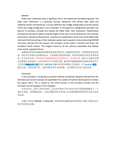
AbstractSlider-crank mechanism plays a significant role in the mechanical manufacturing areas. The slider crank mechanism is a particular four-bar mechanism that exhibits both linear and rotational motion simultaneously. It is also called four-bar linkage configurations and the analysis of four bar linkage configuration is very important. In this paper four configurations are taken into account to synthesis, simulate and analyse the offset slider crank mechanism. Mathematical formulae are derived for determining the lengths of the crank and connecting rod; the kinematic and dynamic analyses of the positions, velocities and accelerations of the links of the offset slider crank and the forces acting on them leading to sparse matrix equation to be solved using MATLAB m-function derived from the analysis; the simulation of the model in Simulink and finally, the simulation results analysis. This program solves for all the unknown parameters and displays those results in graphical forms.曲柄滑块机构在机械制造领域发挥着重要的作用。
Matlab求解理论力学问题系列(二)典型机构的运动分析
—血內 sin(pi — «3^2 sin 巾 一QiS sin 0 = 0 ]
恋91 COS0 +COS02 + 如30 COS0 = 0
〉(5) j
由于0,0,02已在前面求出,因此得到关于內,02 的一组线性方程组。类似X=inv(A)*B可解出角速 度,从而可以获得角速度随时间或随6变化的关系 (图 5)。
步骤(4):类似一元函数的泰勒展开式,= f(xo) + f'(xo){x — X0) + o(x — ®0)> 多兀函数为
fi(x) = f,(x*) + J(x*)dx + o(dx)
1 Matlab中非线性方程的求解及动画演示
案例1:如图1,已知四连杆机构ABCD, AB 杆长为如,BC杆长为a2, CD杆长为a3, AD距离 为cm。若AB杆以匀角速度5转动,初始d0 = Oo 求BC和CD杆的角度、角速度变化规律。
编程计算得到角度的变化关系后,可以算出任 意时刻各较的位置,以及BC杆上不同点的运动轨 迹(图3):很明显B点轨迹是圆,C点轨迹是圆的 一部分(AB杆大范围运动时,CD杆只在小范围运 动),而在BC杆上不同的点轨迹就很复杂了。
各较点的位置并连接起来,就得到了四连杆机构在 某一时刻的图象,延迟一定的时间后再画出下一时 刻的图象,就形成了动画。本问题中动画的源代码 见图4,其中plot函数表示画线段;hl是句柄,定义
ai COS & + Q2 COS 01 + Q3 COS(P2 — «4 = 0 1 ⑴
ai sin 9 + 恋 sin 休 + sin 0 = 0
J
方程(1)是关于转角0和02的非线性方程组,通 常没有解析解,下面给出一般的处理方法。
matlab曲柄连杆机构分析讲课讲稿
m a t l a b曲柄连杆机构分析clear;clc;n=750;l=0.975;R=0.0381;h=0.2;omiga=n.*pi/30;tmax=2.*pi/omiga;t=0:0.001:tmax; %计算曲柄转一圈的总t值alpha1=atan((h+R.*sin(omiga.*t))./sqrt(l.*l-(h+R.*sin(omiga.*t))))+pi;alpha1p=-(R.*omiga.*cos(omiga.*t))./(l.*cos(alpha1));vb=-R.*omiga.*sin(omiga.*t)+R.*omiga.*cos(omiga.*t).*tan(alpha1);ab=-R.*omiga.^2.*cos(omiga.*t)-(R.*omiga.*cos(omiga.*t)).^2./(l.*(cos(alpha1)).^3)-R.*omiga.^2.*sin(omiga.*t).*tan(alpha1);subplot(1,2,1);plot(t,vb);title('曲柄滑块机构的滑块v-t图');xlabel('时间t(曲柄旋转一周)');ylabel('滑块速度v');grid on;subplot(1,2,2);plot(t,ab);title('曲柄滑块机构的滑块a-t图');xlabel('时间t(曲柄旋转一周)');ylabel('滑块加速度a');grid on;%下面黄金分割法求滑块的速度与加速度最大值epsilon=input('根据曲线初始区间已确定,请输入计算精度epsilon(如输入0.001):');a=0;b=0.04; %初始区间n1=0; %n1用于计算次数a1=b-0.618*(b-a);y1=-R.*omiga.*sin(omiga.*a1)+R.*omiga.*cos(omiga.*a1).*tan(alpha1);a2=a+0.618*(b-a);y2=-R.*omiga.*sin(omiga.*a2)+R.*omiga.*cos(omiga.*a2).*tan(alpha1);while abs(a-b)>=epsilonif y1<=y2b=a2;a2=a1;y2=y1;a1=b-0.618*(b-a);y1=-R.*omiga.*sin(omiga.*a1)+R.*omiga.*cos(omiga.*a1).*tan(alpha1);elsea=a1;a1=a2;y1=y2;a2=a+0.618*(b-a);y2=-R.*omiga.*sin(omiga.*a2)+R.*omiga.*cos(omiga.*a2).*tan(alpha1);endn1=n1+1;endvbm1=omiga*(a+b)/2;disp(['经过',num2str(n1),'次计算,用黄金分割法找到速度最大值对应的wt是:', num2str(vbm1),'弧度。
- 1、下载文档前请自行甄别文档内容的完整性,平台不提供额外的编辑、内容补充、找答案等附加服务。
- 2、"仅部分预览"的文档,不可在线预览部分如存在完整性等问题,可反馈申请退款(可完整预览的文档不适用该条件!)。
- 3、如文档侵犯您的权益,请联系客服反馈,我们会尽快为您处理(人工客服工作时间:9:00-18:30)。
物理-曲柄滑块机构的运动分析-m a t l a b
子函数
%子函数slider_crank文件
function[theta2,s3,omega2,v3,alpha2,a3]=slider_crank(thet a1,omega1,alpha1,l1,l2,e)
%计算连杆2的角位移和滑块3的线位移
theta2=asin((e-l1*sin(theta1))/l2);
s3=l1*cos(theta1)+l2*cos(theta2);
%计算连杆2的角为速度和滑块的线速度
A=[-l1*sin(theta1),1;-2*cos(theta2),0];
B=[-l1*sin(theta1);l1*cos(theta1)];
omega=A\(omega1*B);
omega2=omega(1);
v3=omega(2);
%计算连杆2的角加速度和滑块3的线加速度
At=[omega2*l2*cos(theta2),0;
omega2*l2*sin(theta2),0];
Bt=[-omega1*l1*cos(theta1);
-omega1*l1*sin(theta1)];
alpha=A\(-At*omega+alpha1*B+omega1*Bt);
alpha2=alpha(1);
a3=alpha(2);
主函数
%住程序slider_crank_main文件
%输入已经知道的数据
clear;
l1=100;
l2=300;
e=0;
hd=pi/180;
du=180/pi;
omega1=10;
alpha1=0;
%调用子函数slider_ank计算曲柄滑块机构位移,速度,加速度
for n1=1:720
theta1(n1)=(n1-1)*hd;
[theta2(n1),s3(n1),omega2(n1),v3(n1),alpha2(n1),a3(n1)]=s lider_crank...
(theta1(n1),omega1,alpha1,l1,l2,e);
end
%位移,速度,加速度和曲柄滑块机构图形输出
figure(l1);
n1=1:720;
subplot(2,2,1); %绘制位移图
[AX,H1,H2]=plotyy(theta1*du,theta2*du,theta1*du,s3);
set(get(AX(1),'ylabel'),'String','连杆角位移/\circ')
set(get(AX(2),'ylabel'),'String','滑块位移/mm')
title('位移线图');
xlabel('曲柄转角\theta_1/\circ')
grid on;
subplot(2,2,2); %绘制速度图
[AX,H1,H2]=plotyy(theta1*du,omega2,theta1*du,v3);
set(get(AX(2),'ylabel'),'String','滑块速度/mm\cdots^{-1}') title('速度线图');
xlabel('曲柄转角\theta_1/\circ')
ylabel('连杆角速度/rad\cdots^{-1}')
grid on;
subplot(2,2,3); %绘制加速度图
[AX,H1,H2]=plotyy(theta1*du,alpha2,theta1*du,a3);
set(get(AX(2),'ylabel'),'String','滑块加速度/mm\cdots^{-2}')
title('加速度线图');
xlabel('曲柄转角\theta_1/\circ') ylabel('连杆加速度/rad\cdots^{-2}') grid on;
subplot(2,2,4);%绘曲柄滑块机构图
x(1)=0;
y(1)=0;
x(2)=l1*cos(70*hd);
y(2)=l1*sin(70*hd);
x(3)=s3(70);
y(3)=e;
x(4)=s3(70);
y(4)=0;
x(5)=0;
y(5)=0;
x(6)=x(3)-40;
y(6)=y(3)+10;
x(7)=x(3)+40;
y(7)=y(3)+10;
x(8)=x(3)+40;
y(8)=y(3)-10;
x(9)=x(3)-40;
y(9)=y(3)-10;
x(10)=x(3)-40;
y(10)=y(3)+10;
i=1:5;
plot(x(i),y(i));
grid on;
hold on;
i=6:10;
plot(x(i),y(i));
title('曲柄滑块机构');
grid on;
hold on;
xlabel('mm');
ylabel('mm')
axis([-50 400 -20 130]);
plot(x(1),y(1),'o');
plot(x(2),y(2),'o');
plot(x(3),y(3),'o');
%曲柄滑块的仿真运动
figure(2)
m=moviein(20);
j=0;
for n1=1:5:360
j=j+1;
clf;
%
x(1)=0;
y(1)=0;
x(2)=l1*cos(n1*hd); y(2)=l1*sin(n1*hd); x(3)=s3(n1);
y(3)=e;
x(4)=(l1+l2+50);
y(4)=0;
x(5)=0;
y(5)=0;
x(6)=x(3)-40;
y(6)=y(3)+10;
x(7)=x(3)+40;
y(7)=y(3)+10;
x(8)=x(3)+40;
y(8)=y(3)-10;
x(9)=x(3)-40;
y(9)=y(3)-10;
x(10)=x(3)-40;
y(10)=y(3)+10;
%
i=1:3;
plot(x(i),y(i));
grid on;
hold on;
i=4:5;
plot(x(i),y(i));
i=6:10;
plot(x(i),y(i));
plot(x(1),y(1),'o');
plot(x(2),y(2),'o');
plot(x(3),y(3),'o');
xlabel('mm');
ylabel('mm')
axis([-50 450 -150 150]); m(j)=getframe;
end
movie(m)。