风电场疲劳可靠性及有效湍流模型(丹麦)
基于湍流强度分布进行机组疲劳累积的方法探讨
54 风能 Wind Energy基于湍流强度分布进行机组疲劳累积的方法探讨*文 | 蔡继峰,朱瑾,王丹丹根据国家发展改革委发布的《关于完善风电上网电价政策的通知》,风电即将迎来平价时代,为此,风电产业需要从全生命周期各个环节挖掘降本增效的空间。
以风电机组设计为例,在进行机组设计时常常会由于不确定性或者为了简化设计而采用保守处理的方式,因此,对机组设计进行优化,可能是未来降本降载的一个方向。
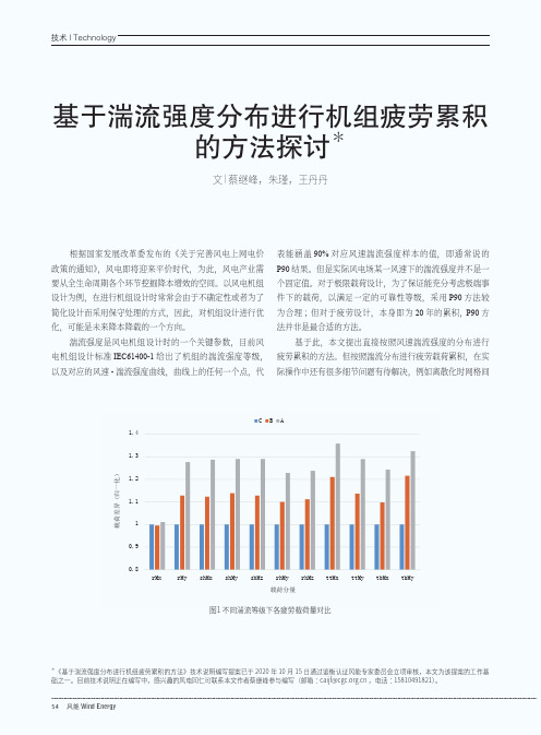
湍流强度是风电机组设计时的一个关键参数,目前风电机组设计标准IEC61400-1给出了机组的湍流强度等级,以及对应的风速-湍流强度曲线,曲线上的任何一个点,代表能涵盖90%对应风速湍流强度样本的值,即通常说的P90结果。
但是实际风电场某一风速下的湍流强度并不是一个固定值。
对于极限载荷设计,为了保证能充分考虑极端事件下的载荷,以满足一定的可靠性等级,采用P90方法较为合理;但对于疲劳设计,本身即为20年的累积, P90方法并非是最合适的方法。
基于此,本文提出直接按照风速湍流强度的分布进行疲劳累积的方法。
但按照湍流分布进行疲劳载荷累积,在实际操作中还有很多细节问题有待解决,例如离散化时网格间*《基于湍流强度分布进行机组疲劳累积的方法》技术说明编写提案已于2020年10月15日通过鉴衡认证风能专家委员会立项审核,本文为该提案的工作基础之一。
目前技术说明正在编写中,感兴趣的风电同仁可联系本文作者蔡继峰参与编写(邮箱::。
图1 不同湍流等级下各疲劳载荷量对比1.41.31.21.110.90.8载荷差异(归一化)CB ArMx rMy shMx shMy shMz rhMy rhMz ttMx ttMy tbMx tbMy载荷分量2020年第12期 55(a) 叶根My等效疲劳载荷(b) 塔顶My等效疲劳载荷(c) 塔底My等效疲劳载荷 图2 等效疲劳载荷随湍流强度变化关系湍流强度(%)等效疲劳载荷(k N .m )6000500040003000200010000.0 5.0 10.0 15.0 20.0 25.0y =187.57x +1099.8R 2=0.9949湍流强度(%)等效疲劳载荷(k N .m )0.0 5.0 10.0 15.0 20.0 25.0y =84.941x +262.78R 2=0.99582500200015001000500等效疲劳载荷(k N .m )湍流强度(%)0.0 5.0 10.0 15.0 20.0 25.0y =571.82x +906R 2=0.99251400012000100008000600040002000隔选取、每个区间代表湍流强度的确定等。
风力机尾流模拟国内外发展概况
风力机尾流模拟国内外发展概况气流通过旋转的风力机转子时产生动量损失,会在风力机下游形成风速下降的区域,该区域被称为尾流区。
尾流的紊流结构会影响下游风力机的疲劳载荷,使风力机的性能受到影响,功率输出减小,导致整个风电场的总功率输出受到影响。
1979年,Lissaman在瑞典Kalkugen实测数据的基础上,基于湍流喷射的相似理论,提出了单风力机尾流的计算模型—Lissaman模型。
继Lissaman模型之后,1986年,丹麦Riso的Katic等提出了Park模型,并将其应用到风能资源评估软件WAsP 中。
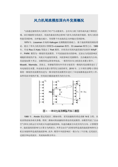
PARK 模型为一维线性尾流模型,不考虑湍流效应的影响,近似认为尾流影响区域随距离线性扩张,风轮后风速线性恢复,风轮影响区是圆锥形,且沿截面均匀分布,其流场如图1所示。
该模型的运算效率较高,一般常用在风力机优化布置计算中。
Mosetti、Marmidis、苏勋文、郑睿敏等国内外学者分别采用一维线性尾流模型进行了风电场优化布置、风电场发电量计算等发方面的研究。
2010年,王丰利用CFD计算结果将一维线性尾流模型改进为一维非线性尾流模型并进行了风电场微观选址研究工作,虽然尾流非线性扩展,但尾流区截面速度仍为均匀分布。
1988年,Ainslie假定尾流区二维轴对称,采用涡漩粘性理论求解N-S方程,从而求得流场各相关参数,得到二维轴对称涡漩粘性理论的尾流模型,该模型考虑了自由空气和风力机运行对风轮后风速的湍流影响,风速沿截面方向是非均匀分布。
计算模型中,湍流强度的影响与计算分为两部分:外界自由空气的剪切所造成的湍流影响和风力机自身旋转所造成的湍流影响。
此外,模型中风轮影响区一般分为三个区域:近尾流区、过渡区和远尾流区,其流场如图2所示。
各区域边界条件计算方法各不相同,如GH模型中近尾流区长度假设为2倍风轮直径,UO模型和FLaP模型则根据经验公式计算得到。
该模型运算较为复杂,效率较低,但计算精度相对高,一般常用于流场与风力机发电量的精确计算。
风电叶片结构疲劳状态智能评估与预警

风电叶片结构疲劳状态智能评估与预警随着社会对可再生能源需求的增加,风能作为一种重要的清洁能源正日益受到重视。
风电叶片作为风力发电机组的核心部件,其疲劳状态的评估与预警显得尤为重要。
本文将介绍风电叶片结构的疲劳状况智能评估与预警技术。
一、风电叶片疲劳状态评估的重要性及背景风电叶片在长期的运行过程中会承受风力带来的巨大压力和振动,容易导致疲劳破坏。
疲劳破坏的发生不仅可能导致风电叶片的损坏,还会造成安全隐患和能源损失。
因此,准确评估风电叶片的疲劳状态,采取有效的预警措施对于保障风电系统的稳定运行至关重要。
二、风电叶片疲劳状态评估方法1. 传统方法:传统的风电叶片疲劳状态评估方法主要依靠人工检查和设备监测。
人工检查需要大量的时间和人力,并且无法实现对风电叶片内部结构的全面评估。
设备监测虽然能够实时监测叶片的振动和温度等参数,但对于疲劳损伤的评估仍然有一定的局限性。
2. 基于数据分析的方法:随着大数据和人工智能的兴起,基于数据分析的风电叶片疲劳状态评估方法逐渐成为研究的热点。
这种方法通过采集大量的风电叶片运行数据,并应用数据挖掘和机器学习等技术,建立疲劳状态评估模型,可实现对叶片结构的智能评估和预警。
三、风电叶片疲劳状态预警技术1. 基于振动信号的预警技术:风电叶片在运行过程中会产生一定的振动信号,这些振动信号包含了叶片结构的重要信息。
利用振动信号分析技术,可以提取叶片的振动特征,进而判断叶片是否存在疲劳损伤,并进行预警。
2. 基于温度变化的预警技术:叶片在风力作用下产生摩擦,会导致温度的变化。
利用温度传感器等设备,实时监测叶片温度的变化情况,当温度异常升高时,可能意味着叶片存在疲劳损伤,并及时进行预警。
3. 基于机器学习的预警技术:机器学习技术能够从海量的数据中学习和发现规律,并进行预测和判断。
通过对大量的风电叶片运行数据进行学习和训练,可以建立预测模型,实现对叶片疲劳状态的预警。
四、风电叶片疲劳状态智能评估与预警的挑战与展望1. 数据获取问题:风电叶片的运行数据获取面临一定的困难和挑战,如数据采集设备的设置和维护问题等。
海上风机基础结构的疲劳及其可靠性研究现状
· 172·
State of the Art
N 曲线法得到的要 法得到的疲劳寿命通常比 S短。但是当结构构件承受较高的应力水平时, 疲 可用断裂 劳开裂阶段寿命占总寿命的比重较小, 力学方法计算得到更真实的疲劳寿命 。 按照计算疲劳损伤参量的不同可以将疲劳寿 命分析方法分为: 名义应力法、 能量法、 应力应变 场强度法、 功率谱密度法等。实际上, 各种方法适 , 用于不同阶段 故选用不同计算方法的组合即形 N 曲线 成了计算疲劳全寿命的不同模式, 包括 S损失力学法与断裂力学 法加断裂力学法的模式、 法相结合的模式、 局部应力—应变法加断裂力学 [2 ] 的模式以及损失力学模式共四种 。 对应不同的 工程选用合适的模型是估算结构疲劳寿命的关键所 这也是目前需要进一步开展研究的重要课题。 在, API 规范[3]指出, 对导管架型结构需要进行 详细的疲劳分析, 建议采用谱分析方法; 对在水深 用韧性钢材建造、 具有高超静 小于 122 m 的水中, 定自由度构架的、 自振周期小于 3 s 的导管架型 平台的管节点可应用简化的疲劳寿命分析方法 。 吴芳和 根据 API 规范中相应的要求, 考虑风浪 , N曲 流引起的疲劳载荷 通过简单疲劳分析法 ( S[4 ]
据和冰激振动理论, 提出了针对不同的海冰破坏 形式, 如挤压、 屈曲、 弯曲等, 分别计算管节点的疲 再进行叠加以得出其等效应力幅的 劳累计损伤, 该方法同时考虑了冰载相对时间和冰厚的 新方法, 随机性, 较一般采用的单一计算方法更为精确可靠。 选用分析海上风机基础结构的方法应该根据 不同的工况来确定, 但不管是哪种分析方法, 疲劳 寿命的估算都包含以下三部分的内容: ① 材料疲 劳行为的描述; ②循环载荷下结构的响应; ③疲劳 累积损伤法则。 2. 2 风波联合作用及波浪模型的选择
考虑疲劳载荷的风电场分散式频率响应策略

考虑疲劳载荷的风电场分散式频率响应策略
杨伟峰;文云峰;李立;王康;迟方德;张武其
【期刊名称】《电力自动化设备》
【年(卷),期】2022(42)4
【摘要】风电场参与调频时会增加风机的疲劳载荷,导致风电场维护成本上升、运营效益下降。
为此,提出一种考虑疲劳载荷的风电场分散式频率响应策略,可在维持
风电场调频性能的同时,降低风机疲劳损伤。
为实现该目标,首先分析风电场调频及
有功控制结构,推导风机线性动力学模型,并构建考虑疲劳载荷的单机频率响应模型。
然后基于Jensen尾流模型,推导风电场由尾流波动产生疲劳载荷的解析式,并结合
单机模型构建风电场频率响应模型。
为减少风电场中央控制器计算压力,采用目标
级联分析法将原集中式优化问题拆分成主问题(中央控制器)和多个子问题(本地控
制器),建立分散式频率响应策略。
最后在MATLAB/Simulink中搭建含80台单机
容量为5 MW双馈风机的IEEE RTS-79系统,并通过仿真验证所提策略的有效性。
【总页数】8页(P55-62)
【作者】杨伟峰;文云峰;李立;王康;迟方德;张武其
【作者单位】湖南大学电气与信息工程学院;国网陕西省电力公司电力调度控制中
心
【正文语种】中文
【中图分类】TM614
【相关文献】
1.航空发动机疲劳载荷分散性及其对应的疲劳分散系数研究
2.考虑多无功源的分散式风电场多时间尺度无功协调控制
3.分散式风电场DFIG与SVC协调无功控制策略
4.考虑尾流效应与载荷损耗的风电场优化控制
5.考虑载荷抑制的风电场分布式自动发电控制
因版权原因,仅展示原文概要,查看原文内容请购买。
基于概率密度演化的风机基础疲劳可靠度计算

基于概率密度演化的风机基础疲劳可靠度计算作者:赵俭斌王凯威王一达付兵来源:《湖南大学学报·自然科学版》2020年第09期摘要:風机底部基础在风荷载作用下会产生疲劳破坏.为了研究风荷载作用下风机的疲劳可靠性,将随机脉动风荷载进行正交展开,用数论选点法和概率密度演化方法将展开的风荷载模型用于风机塔身的疲劳可靠度计算.采用推力系数法计算风荷载作用下风机基础较危险部位的应力时程,然后用雨流计数法统计该点的疲劳损伤,将其代入概率密度演化方程并通过差分计算可求得疲劳损伤的概率密度函数.通过累计疲劳损伤小于1的概率可求得危险部位的疲劳可靠度,也就是整个基础的疲劳可靠度.以一3 MW风机作为算例验证了本文方法的有效性,应用概率密度演化方法,可以精确地给出基础在风荷载作用下的疲劳可靠度,本文成果对于近似工况的风机基础疲劳可靠度的计算具有借鉴意义.关键词:风机;概率密度演化;疲劳可靠度;正交展开;雨流计数法中图分类号:TU359;TM614 文献标志码:A文章编号:1674—2974(2020)09—0120—08Abstract:The bottom of wind turbine foundation will cause fatigue damage under wind loads. In order to study the fatigue reliability of wind turbines under wind loads, the random fluctuating wind loads were expanded orthogonally, and the expanded wind load model was used to calculate the fatigue reliability of the wind turbine tower using the number theory selection method and the probability density evolution method. The thrust coefficient method was used to calculate the stress time history of the dangerous part of the wind turbine foundation under the wind load, and then thefatigue damage of the point was calculated by the rain flow counting method, which is substituted into the probability density evolution equation. The probability density function of fatigue damage can be obtained by solving differential equation. By accumulating the probability of fatigue damage less than 1, the fatigue reliability of the dangerous parts can be obtained, that is, the fatigue reliability of the entire foundation. The effectiveness of the proposed method is verified by a 3 MW wind turbine. Using the probability density evolution method, the fatigue reliability of the foundation under wind load can be accurately given. The findings of this paper have reference significance for the calculation of fatigue reliability of wind turbine foundation under similar working conditions.Key words:wind turbine;probability density evolution;fatigue reliability;orthogonal expansion;rain flow counting在过去20年,风电持续高速发展[1-3],到2018年底,全球风电累计装机容量已突破600 GW,新增装机容量共53.9 GW.风机受到长期的动力荷载作用,疲劳问题突出,需要准确预测风机结构的疲劳损伤,尤其是在塔底动应力很高的地方.影响结构疲劳损伤的因素甚多,其中荷载是最主要的方面,风荷载本质上具有不可忽略的随机性,因此,采用可靠度的分析方法分析结构疲劳损伤是一种自然的选择.目前,可靠度的求解方法包括:Monte Carlo[4,5]、一次二阶矩[5]、响应面法[5]等. 基于一次二阶矩理论的可靠度分析方法的主要目标在于寻求随机结构响应的二阶矩统计量. 在获得二阶矩统计量之后,通过假定结构响应服从正态分布计算结构的使用可靠度.响应面法的基本思想是将功能函数的输入和输出变量表示为标准正态分布变量的多项式,而各变量的系数通过配点法(collocation points)确定,最后由功能方程得到可靠指标和失效概率.Monte Carlo法虽然适用性较强,但以过高的计算量为代价. 近年来陈建兵和李杰[7-9]发展了一类随机结构反应的概率密度演化方法,利用这种方法,可以精确定量地给出结构反应的演化概率密度曲线族,由此,可方便地根据指定的位移反应限值,直接计算给出随机结构在随机荷载作用下的可靠度.对于风机这种新的结构形式,其受到的风荷载突出,随机风引起的疲劳损伤问题也更突出,但是有关风机结构的疲劳可靠度分析成果还很少.本文基于概率密度演化思想,构造一个虚拟随机过程,使得随机结构时域内的疲劳损伤为该虚拟随机过程的截口随机变量. 进而,建立概率密度演化方程并求解出随机结构疲劳损伤的概率密度,在安全域内积分给出结构的疲劳可靠度.1 风荷载的数值模拟设x,y,z为空间中的一个点,其中z是离地面的高度,x是横向风向,y是顺风向.在实践中,为了简化概念,风速波动可以在平面y=0中表征[10]. 当只考虑竖向相关性时,风速场可以写成:2 疲劳可靠度分析的概率密度演化方法在对风速进行正交展开后,可将展开结果代入塔身动力反应控制方程,求解控制方程进而可以得到对应不同θ的动力反应(如塔身某点的速度),将对应于不同θ的动力反应代入概率密度演化方程,将求解结果对θ积分,可得所需要的动力反应随时间变化的概率密度.风机结构的动力反应控制方程[14]为:对于疲劳损伤D,就结构动力学问题而言,它必连续依赖于随机参数θ,构造以τ为虚拟时间参数的虚拟随机过程Zl3 疲劳累积损伤理论损伤是指在循环荷载作用下材料的损坏程度,一般用一个无量纲参数D来表示它,当D = 0时,说明材料完好无损,当D > 1时,表示材料已经达到它的疲劳寿命.在随机荷载作用下,结构疲劳损伤分析采用疲劳累积损伤理论. 目前普遍采用的理论有Palmgren[20]-Miner[21]线性疲劳损伤准则.本文主要分析风荷载作用下风机塔身底部混凝土基础的疲劳可靠度,采用P-M准则对应的S-N曲线[22]为:式中:Smax为风荷载作用下的应力范围,单位为MPa,Nf为对应Smax的导致材料发生疲劳破坏的循环次数.疲劳损伤D的定义为式中:nk为第k级应力幅值下的实际循环次数,Nf k为第k级应力幅值下达到疲劳破坏时的允许循环次数,由S-N曲线查得. k为计算疲劳损伤时所涉及到的所有工况所对应的应力幅值总数.4 实例计算本文基于某风电场3 MW风力发电机进行建模分析.该风力发电机轮毂高度90 m,风轮直径100.8 m,额定风速11.9 m/s,设计寿命为20年. 基础混凝土采用圆形台柱式扩展基础,底板直径21.5 m,高3.9 m,埋深3.5 m. 塔筒材料为Q345钢材,基础环采用Q345钢材,基础混凝土采用C35混凝土,底部采用完全约束,采用ABAQUS有限元软件建立模型,选用实体单元.表1为各段塔筒的几何参数,采用的ABAQUS中混凝土损伤本构模型如图1所示.图1中,fcm为屈服强度,εc1为屈服应变,Ec为弹性模量,dc为损伤因子,εinc 为非线性应变,εplc 为塑形应变,εelc 为弹性应变,σc为压应力,εc为压应变,dc = (1 - βc)εinc Ec /σc +(1 - βc)εinc Ec,βc取值为0.35~0.7,应力应变关系由混凝土规范[23]提供,将相关参数输入软件中计算可得所需数据.4.1 风荷载的计算平均风速的选取考虑到轮毂处的工作情况,根据平均风速的指数模型计算可选取相应10 m处平均风速(标准平均风速)12 m/s.在计算方程(18)时,令θ = θq,θq = (θ1,q,θ2,q,…,θs,q)(s = 15,q = 1,2,…,Nsel),将对应θq的D(θq,T)代入方程中,可得联合概率密度函数p zl Θ(z,θq,τ),进而对方程(20)积分并结合式(21)和(22),最终可得D值的疲劳可靠度.关于Nsel的选取遵循数论选点法,在Matlab中实现选取步骤,对n = 2 422 957的随机列向量采用数论选点法[10,15,16]进行筛选,得到Nsel = 182个随机列向量组,依次编号1、2、3…,方便后续整理计算.在这182个随机列向量组的基础上,根据算法在Matlab中进行编程,独立地生成标准平均风速为12 m/s时的182种风速时间历程,每一个随机列向量对应生成一个风速时程,将脉动风速时程继承随机列向量的编号,并将脉动风时程与平均风时程合并,可得到轮毂处的总风速时程,如图2.为了验证风速模拟数值的准确性,在平均风速为10.27 m/s时进行实测,实测风速的采样频率为1/7 Hz,选择的实测风速为风向稳定且基本与应变测点一致的时间段,实测结果如图3. 采用文中所述方法展开风速为10.27 m/s时结果如图4.由对比可知,文中风速展开方法与实测值趋势大体一致,可以由此确定风速模拟取值的正确性.4.2 风机动力响应的有限元模拟将风荷载时程加载至风机模型上,可以得到各个随机风荷载下的风机动力响应,本文主要观察钢环与混凝土接触范围内的动力响应,取10 m处平均风速为12 m/s.利用公式(14)、(15)计算塔身处各点的风荷载时程.将风荷载加至有限元模型,并考虑塔身风荷载的影响,采用应力等值线来表示模型内部的应力分布情况,可以清晰描述外动力响应在结构中的分布,从而快速确定模型中的最危險区域.疲劳损伤的计算是在等效应力时程的基础上计算,因此提取基础环和基础的等效应力云图.本文提取182种随机风荷载时程的第一和第二个时程,编号为1、2,编号1、2动力响应下基础环和基础等效应力云图如图5所示.对于风机这种新的结构形式,其受到的风荷载突出,随机风引起的疲劳损伤问题也更突出,但是有关风机结构的疲劳可靠度分析成果还很少.本文基于概率密度演化思想,构造一个虚拟随机过程,使得随机结构时域内的疲勞损伤为该虚拟随机过程的截口随机变量. 进而,建立概率密度演化方程并求解出随机结构疲劳损伤的概率密度,在安全域内积分给出结构的疲劳可靠度.1 风荷载的数值模拟设x,y,z为空间中的一个点,其中z是离地面的高度,x是横向风向,y是顺风向.在实践中,为了简化概念,风速波动可以在平面y=0中表征[10]. 当只考虑竖向相关性时,风速场可以写成:2 疲劳可靠度分析的概率密度演化方法在对风速进行正交展开后,可将展开结果代入塔身动力反应控制方程,求解控制方程进而可以得到对应不同θ的动力反应(如塔身某点的速度),将对应于不同θ的动力反应代入概率密度演化方程,将求解结果对θ积分,可得所需要的动力反应随时间变化的概率密度.风机结构的动力反应控制方程[14]为:对于疲劳损伤D,就结构动力学问题而言,它必连续依赖于随机参数θ,构造以τ为虚拟时间参数的虚拟随机过程Zl3 疲劳累积损伤理论损伤是指在循环荷载作用下材料的损坏程度,一般用一个无量纲参数D来表示它,当D = 0时,说明材料完好无损,当D > 1时,表示材料已经达到它的疲劳寿命.在随机荷载作用下,结构疲劳损伤分析采用疲劳累积损伤理论. 目前普遍采用的理论有Palmgren[20]-Miner[21]线性疲劳损伤准则.本文主要分析风荷载作用下风机塔身底部混凝土基础的疲劳可靠度,采用P-M准则对应的S-N曲线[22]为:式中:Smax为风荷载作用下的应力范围,单位为MPa,Nf为对应Smax的导致材料发生疲劳破坏的循环次数.疲劳损伤D的定义为式中:nk为第k级应力幅值下的实际循环次数,Nf k为第k级应力幅值下达到疲劳破坏时的允许循环次数,由S-N曲线查得. k为计算疲劳损伤时所涉及到的所有工况所对应的应力幅值总数.4 实例计算本文基于某风电场3 MW风力发电机进行建模分析.该风力发电机轮毂高度90 m,风轮直径100.8 m,额定风速11.9 m/s,设计寿命为20年. 基础混凝土采用圆形台柱式扩展基础,底板直径21.5 m,高3.9 m,埋深3.5 m. 塔筒材料为Q345钢材,基础环采用Q345钢材,基础混凝土采用C35混凝土,底部采用完全约束,采用ABAQUS有限元软件建立模型,选用实体单元.表1为各段塔筒的几何参数,采用的ABAQUS中混凝土损伤本构模型如图1所示.图1中,fcm为屈服强度,εc1为屈服应变,Ec为弹性模量,dc为损伤因子,εinc 为非线性应变,εplc 为塑形应变,εelc 为弹性应变,σc为压应力,εc为压应变,dc = (1 - βc)εinc Ec /σc +(1 - βc)εinc Ec,βc取值为0.35~0.7,应力应变关系由混凝土规范[23]提供,将相关参数输入软件中计算可得所需数据.4.1 风荷载的计算平均风速的选取考虑到轮毂处的工作情况,根据平均风速的指数模型计算可选取相应10 m处平均风速(标准平均风速)12 m/s.在计算方程(18)时,令θ = θq,θq = (θ1,q,θ2,q,…,θs,q)(s = 15,q = 1,2,…,Nsel),将对应θq的D(θq,T)代入方程中,可得联合概率密度函数p zl Θ(z,θq,τ),进而对方程(20)积分并结合式(21)和(22),最终可得D值的疲劳可靠度.关于Nsel的选取遵循数论选点法,在Matlab中实现选取步骤,对n = 2 422 957的随机列向量采用数论选点法[10,15,16]进行筛选,得到Nsel = 182个随机列向量组,依次编号1、2、3…,方便后续整理计算.在这182个随机列向量组的基础上,根据算法在Matlab中进行编程,独立地生成标准平均风速为12 m/s时的182种风速时间历程,每一个随机列向量对应生成一个风速时程,将脉动风速时程继承随机列向量的编号,并将脉动风时程与平均风时程合并,可得到轮毂处的总风速时程,如图2.为了验证风速模拟数值的准确性,在平均风速为10.27 m/s时进行实测,实测风速的采样频率为1/7 Hz,选择的实测风速为风向稳定且基本与应变测点一致的时间段,实测结果如图3. 采用文中所述方法展开风速为10.27 m/s时结果如图4.由对比可知,文中风速展开方法与实测值趋势大体一致,可以由此确定风速模拟取值的正确性.4.2 风机动力响应的有限元模拟将风荷载时程加载至风机模型上,可以得到各个随机风荷载下的风机动力响应,本文主要观察钢环与混凝土接触范围内的动力响应,取10 m处平均风速为12 m/s.利用公式(14)、(15)计算塔身处各点的风荷载时程.将风荷载加至有限元模型,并考虑塔身风荷载的影响,采用应力等值线来表示模型内部的应力分布情况,可以清晰描述外动力响应在结构中的分布,从而快速确定模型中的最危险区域.疲劳损伤的计算是在等效应力时程的基础上计算,因此提取基础环和基础的等效应力云图.本文提取182种随机风荷载时程的第一和第二个时程,编号为1、2,编号1、2动力响应下基础环和基础等效应力云图如图5所示.对于风机这种新的结构形式,其受到的风荷载突出,随机风引起的疲劳损伤问题也更突出,但是有关风机结构的疲劳可靠度分析成果还很少.本文基于概率密度演化思想,构造一个虚拟随机过程,使得随机结构时域内的疲劳损伤为该虚拟随机过程的截口随机变量. 进而,建立概率密度演化方程并求解出随机结构疲劳损伤的概率密度,在安全域内积分给出结构的疲劳可靠度.1 风荷载的数值模拟设x,y,z为空间中的一个点,其中z是离地面的高度,x是横向风向,y是顺风向.在实践中,为了简化概念,风速波动可以在平面y=0中表征[10]. 当只考虑竖向相关性时,风速场可以写成:2 疲劳可靠度分析的概率密度演化方法在对风速进行正交展开后,可将展开结果代入塔身动力反应控制方程,求解控制方程进而可以得到对应不同θ的动力反应(如塔身某点的速度),将对应于不同θ的动力反应代入概率密度演化方程,将求解结果对θ积分,可得所需要的动力反应随时间变化的概率密度.风机结构的动力反应控制方程[14]为:对于疲劳损伤D,就结构动力学问题而言,它必连续依赖于随机参数θ,构造以τ为虚拟时间参数的虚拟随机过程Zl3 疲劳累积损伤理论损伤是指在循环荷载作用下材料的损坏程度,一般用一个无量纲参数D来表示它,当D = 0时,说明材料完好无损,当D > 1时,表示材料已经达到它的疲劳寿命.在随机荷载作用下,结构疲劳损伤分析采用疲劳累积损伤理论. 目前普遍采用的理论有Palmgren[20]-Miner[21]线性疲劳损伤准则.本文主要分析风荷载作用下风机塔身底部混凝土基础的疲劳可靠度,采用P-M准则对应的S-N曲线[22]为:式中:Smax为风荷载作用下的应力范围,单位为MPa,Nf为对应Smax的导致材料发生疲劳破坏的循环次数.疲劳损伤D的定义为式中:nk为第k级应力幅值下的实际循环次数,Nf k为第k级应力幅值下达到疲劳破坏时的允许循环次数,由S-N曲线查得. k为计算疲劳损伤时所涉及到的所有工况所对应的应力幅值总数.4 实例计算本文基于某风电场3 MW风力发电机进行建模分析.该风力发电机轮毂高度90 m,风轮直径100.8 m,额定风速11.9 m/s,设计寿命为20年. 基础混凝土采用圆形台柱式扩展基础,底板直径21.5 m,高3.9 m,埋深3.5 m. 塔筒材料为Q345钢材,基础环采用Q345钢材,基础混凝土采用C35混凝土,底部采用完全约束,采用ABAQUS有限元软件建立模型,选用实体单元.表1为各段塔筒的几何参数,采用的ABAQUS中混凝土损伤本构模型如图1所示.图1中,fcm为屈服强度,εc1为屈服应变,Ec为弹性模量,dc为损伤因子,εinc 为非线性应变,εplc 为塑形应变,εelc 为弹性应变,σc为压应力,εc为压应变,dc = (1 - βc)εinc Ec /σc +(1 - βc)εinc Ec,βc取值为0.35~0.7,应力应变关系由混凝土规范[23]提供,将相关参数输入软件中计算可得所需数据.4.1 风荷载的计算平均风速的选取考虑到轮毂处的工作情况,根据平均风速的指数模型计算可选取相应10 m处平均风速(标准平均风速)12 m/s.在计算方程(18)时,令θ = θq,θq = (θ1,q,θ2,q,…,θs,q)(s = 15,q = 1,2,…,Nsel),將对应θq的D(θq,T)代入方程中,可得联合概率密度函数p zl Θ(z,θq,τ),进而对方程(20)积分并结合式(21)和(22),最终可得D值的疲劳可靠度.关于Nsel的选取遵循数论选点法,在Matlab中实现选取步骤,对n = 2 422 957的随机列向量采用数论选点法[10,15,16]进行筛选,得到Nsel = 182个随机列向量组,依次编号1、2、3…,方便后续整理计算.在这182个随机列向量组的基础上,根据算法在Matlab中进行编程,独立地生成标准平均风速为12 m/s时的182种风速时间历程,每一个随机列向量对应生成一个风速时程,将脉动风速时程继承随机列向量的编号,并将脉动风时程与平均风时程合并,可得到轮毂处的总风速时程,如图2.为了验证风速模拟数值的准确性,在平均风速为10.27 m/s时进行实测,实测风速的采样频率为1/7 Hz,选择的实测风速为风向稳定且基本与应变测点一致的时间段,实测结果如图3. 采用文中所述方法展开风速为10.27 m/s时结果如图4.由对比可知,文中风速展开方法与实测值趋势大体一致,可以由此确定风速模拟取值的正确性.4.2 风机动力响应的有限元模拟将风荷载时程加载至风机模型上,可以得到各个随机风荷载下的风机动力响应,本文主要观察钢环与混凝土接触范围内的动力响应,取10 m处平均风速为12 m/s.利用公式(14)、(15)计算塔身处各点的风荷载时程.将风荷载加至有限元模型,并考虑塔身风荷载的影响,采用应力等值线来表示模型内部的应力分布情况,可以清晰描述外动力响应在结构中的分布,从而快速确定模型中的最危险区域.疲劳损伤的计算是在等效应力时程的基础上计算,因此提取基础环和基础的等效应力云图.本文提取182种随机风荷载时程的第一和第二个时程,编号为1、2,编号1、2动力响应下基础环和基础等效应力云图如图5所示.对于风机这种新的结构形式,其受到的风荷载突出,随机风引起的疲劳损伤问题也更突出,但是有关风机结构的疲劳可靠度分析成果还很少.本文基于概率密度演化思想,构造一个虚拟随机过程,使得随机结构时域内的疲劳损伤为该虚拟随机过程的截口随机变量. 进而,建立概率密度演化方程并求解出随机结构疲劳损伤的概率密度,在安全域内积分给出结构的疲劳可靠度.1 风荷载的数值模拟设x,y,z为空间中的一个点,其中z是离地面的高度,x是横向风向,y是顺风向.在实践中,为了简化概念,风速波动可以在平面y=0中表征[10]. 当只考虑竖向相关性时,风速场可以写成:2 疲劳可靠度分析的概率密度演化方法在对风速进行正交展开后,可将展开结果代入塔身动力反应控制方程,求解控制方程进而可以得到对应不同θ的动力反应(如塔身某点的速度),将对应于不同θ的动力反应代入概率密度演化方程,将求解结果对θ积分,可得所需要的动力反应随时间变化的概率密度.风机结构的动力反应控制方程[14]为:对于疲劳损伤D,就结构动力学问题而言,它必连续依赖于随机参数θ,构造以τ为虚拟时间参数的虚拟随机过程Zl3 疲劳累积损伤理论损伤是指在循环荷载作用下材料的损坏程度,一般用一个无量纲参数D来表示它,当D = 0时,说明材料完好無损,当D > 1时,表示材料已经达到它的疲劳寿命.在随机荷载作用下,结构疲劳损伤分析采用疲劳累积损伤理论. 目前普遍采用的理论有Palmgren[20]-Miner[21]线性疲劳损伤准则.本文主要分析风荷载作用下风机塔身底部混凝土基础的疲劳可靠度,采用P-M准则对应的S-N曲线[22]为:式中:Smax为风荷载作用下的应力范围,单位为MPa,Nf为对应Smax的导致材料发生疲劳破坏的循环次数.疲劳损伤D的定义为式中:nk为第k级应力幅值下的实际循环次数,Nf k为第k级应力幅值下达到疲劳破坏时的允许循环次数,由S-N曲线查得. k为计算疲劳损伤时所涉及到的所有工况所对应的应力幅值总数.4 实例计算本文基于某风电场3 MW风力发电机进行建模分析.该风力发电机轮毂高度90 m,风轮直径100.8 m,额定风速11.9 m/s,设计寿命为20年. 基础混凝土采用圆形台柱式扩展基础,底板直径21.5 m,高3.9 m,埋深3.5 m. 塔筒材料为Q345钢材,基础环采用Q345钢材,基础混凝土采用C35混凝土,底部采用完全约束,采用ABAQUS有限元软件建立模型,选用实体单元.表1为各段塔筒的几何参数,采用的ABAQUS中混凝土损伤本构模型如图1所示.图1中,fcm为屈服强度,εc1为屈服应变,Ec为弹性模量,dc为损伤因子,εinc 为非线性应变,εplc 为塑形应变,εelc 为弹性应变,σc为压应力,εc为压应变,dc = (1 - βc)εinc Ec /σc +(1 - βc)εinc Ec,βc取值为0.35~0.7,应力应变关系由混凝土规范[23]提供,将相关参数输入软件中计算可得所需数据.4.1 风荷载的计算平均风速的选取考虑到轮毂处的工作情况,根据平均风速的指数模型计算可选取相应10 m处平均风速(标准平均风速)12 m/s.在计算方程(18)时,令θ = θq,θq = (θ1,q,θ2,q,…,θs,q)(s = 15,q = 1,2,…,Nsel),将对应θq的D(θq,T)代入方程中,可得联合概率密度函数p zl Θ(z,θq,τ),进而对方程(20)积分并结合式(21)和(22),最终可得D值的疲劳可靠度.关于Nsel的选取遵循数论选点法,在Matlab中实现选取步骤,对n = 2 422 957的随机列向量采用数论选点法[10,15,16]进行筛选,得到Nsel = 182个随机列向量组,依次编号1、2、3…,方便后续整理计算.在这182个随机列向量组的基础上,根据算法在Matlab中进行编程,独立地生成标准平均风速为12 m/s时的182种风速时间历程,每一个随机列向量对应生成一个风速时程,将脉动风速时程继承随机列向量的编号,并将脉动风时程与平均风时程合并,可得到轮毂处的总风速时程,如图2.为了验证风速模拟数值的准确性,在平均风速为10.27 m/s时进行实测,实测风速的采样频率为1/7 Hz,选择的实测风速为风向稳定且基本与应变测点一致的时间段,实测结果如图3. 采用文中所述方法展开风速为10.27 m/s时结果如图4.由对比可知,文中风速展开方法与实测值趋势大体一致,可以由此确定风速模拟取值的正确性.4.2 风机动力响应的有限元模拟将风荷载时程加载至风机模型上,可以得到各个随机风荷载下的风机动力响应,本文主要观察钢环与混凝土接触范围内的动力响应,取10 m处平均风速为12 m/s.利用公式(14)、(15)计算塔身处各点的风荷载时程.。
基于大数据与湍流模型的风电场评估与优化
基于大数据与湍流模型的风电场评估与优化随着环保和能源议题日益受到重视,风能作为一种清洁、可再生的能源形式受到越来越多的关注。
风能是目前发展最迅速的新兴能源之一,风能产业正以高速度发展,已经成为可再生能源的核心产业之一。
而风能的利用主要通过风电场实现。
在建设和运营风电站时,对于风场的规划、布局和运营,评估与优化显得尤为重要,对提高风电场的发电效率和降低运营成本具有重要意义。
在评估与优化风电场的过程中,大数据技术和湍流模型成为了不可或缺的工具。
一、大数据在风电场评估中的应用大数据是指海量的结构化、半结构化和非结构化数据,随着科技的发展和数字化转型的深入,大数据已经在许多领域发挥了巨大的作用。
在风电场的评估和优化中,大数据的应用也越来越得到关注。
首先,风电场的运营涉及到很多方面的数据记录和处理,包括风速、风向、温度、湿度等的收集和分析。
传统的数据处理方法已经无法满足大规模数据的处理和分析需要,因此需要利用大数据技术对海量的数据进行处理和分析,从而在风电场的规划、建设和运营过程中提高效率、降低成本、节约资源。
例如,利用大数据分析技术可以对风能资源进行评估,优化风电场的选址和布局;利用大数据分析技术可以对风电场的结构、技术参数等进行分析和优化,提高发电效率和运营稳定性。
其次,利用大数据技术可以实现风电场的智能化运营。
通过智能化监测和控制系统,可以对风电场的运行状态进行实时监测和控制,及时发现和解决各种故障,并对风场进行远程管理和调度。
此外,利用大数据技术还可以对风电场的供应链进行管理和优化,从而提高风电场的整体运作效率。
二、湍流模型在风电场评估中的应用湍流是一种复杂的流动状态,其中涡旋流动会对风力发电机叶轮产生影响,进而影响发电量和稳定性。
因此,在风电场的建设和运营中,对湍流进行建模和模拟,评估湍流影响对风电发电的影响显得尤为重要。
湍流模型是针对湍流流动特性进行建模和仿真的一种技术。
通过对湍流流动进行准确的建模和仿真,可以对风电场的发电量和稳定性进行评估和优化。
大气工程中风力发电塔筒结构的疲劳性能评估

大气工程中风力发电塔筒结构的疲劳性能评估随着风力发电的快速发展,塔筒结构作为一个关键组成部分,有着重要的作用。
然而,在长期的风力作用下,塔筒结构容易出现疲劳破坏,影响风力发电的正常运行。
因此,对于风力发电塔筒结构的疲劳性能进行评估,具有重要的意义。
首先,我们需要了解什么是疲劳破坏。
疲劳破坏是指在循环载荷作用下,结构在未达到其静力强度的情况下发生破坏。
疲劳破坏是一种逐渐发展的过程,通常起始于微小的裂纹,然后沿着应力最大的位置扩展,最终导致结构破裂。
因此,疲劳性能评估的关键是确定结构中的疲劳破坏起始位置和扩展情况。
在风力发电塔筒结构的疲劳性能评估中,我们需要考虑到以下几个因素。
首先是塔筒结构的材料性能。
不同材料的疲劳特性存在差异,因此需要根据具体的材料选取合适的疲劳参数。
其次是结构的设计参数,包括截面尺寸、连接方式等。
这些设计参数会对结构的应力分布产生影响,从而影响疲劳寿命。
最后是外界环境因素,如风速、震动等。
这些因素会对塔筒结构产生不同程度的影响。
疲劳性能评估的方法主要包括实验研究和数值模拟两种。
实验研究通过在实验室中进行长期循环载荷试验,来模拟结构在实际运行条件下的疲劳行为。
这种方法对于验证理论模型和分析方法具有重要的作用。
然而,实验研究的成本较高且时间较长,无法涵盖所有的工况和边界条件。
因此,数值模拟成为研究人员常用的手段。
数值模拟采用计算机辅助工程软件,根据塔筒结构的几何形状和材料性能,通过有限元分析等方法,来模拟结构在不同工况下的应力分布和疲劳寿命。
数值模拟具有高效、经济和便捷的优点,可以在短时间内预测结构的疲劳性能。
疲劳性能评估的结果可以用疲劳寿命和安全系数来表示。
疲劳寿命是指结构在疲劳载荷下的使用年限,通常以循环数表示。
安全系数是指设计疲劳载荷与疲劳破坏强度之间的比值。
当安全系数大于1时,表示结构的设计寿命大于使用寿命,具有足够的安全性。
而当安全系数小于1时,表示结构的设计寿命小于使用寿命,存在疲劳破坏的风险。
- 1、下载文档前请自行甄别文档内容的完整性,平台不提供额外的编辑、内容补充、找答案等附加服务。
- 2、"仅部分预览"的文档,不可在线预览部分如存在完整性等问题,可反馈申请退款(可完整预览的文档不适用该条件!)。
- 3、如文档侵犯您的权益,请联系客服反馈,我们会尽快为您处理(人工客服工作时间:9:00-18:30)。
Applications of Statistics and Probability in Civil Engineering–Kanda,Takada&Furuta(eds)©2007Taylor&Francis Group,London,ISBN978-0-415-45211-3 Fatigue reliability and effective turbulence models in wind farmsJ.D.SørensenAalborg University,Aalborg,DenmarkRisøNational Laboratory,Roskilde,DenmarkS.Frandsen&N.J.Tarp-JohansenRisøNational Laboratory,Roskilde,DenmarkABSTRACT:Offshore wind farms with100or more wind turbines are expected to be installed many places during the next years.Behind a wind turbine a wake is formed where the mean wind speed decreases slightly and the turbulence intensity increases significantly.This increase in turbulence intensity in wakes behind wind turbines can imply a significant reduction in the fatigue lifetime of wind turbines placed in wakes.In this paper the design code model in the wind turbine code IEC61400-1(2005)is evaluated from a probabilistic point of view,including the importance of modeling the SN-curve by linear or bi-linear models.Further,the influence on the fatigue reliability is investigated from modeling the fatigue response by a stochastic part related to the ambient turbulence and the eigenfrequencies of the structure and a deterministic,sinusoidal part with frequency of revolution of the rotor.1INTRODUCTIONWind turbines for electricity production have increased significantly the last years both in production capa-bility and in size.This development is expected to continue also in the coming years.Offshore wind turbines with an installed capacity of5–10MW are planned.Typically,these large wind turbines are placed in offshore wind farms with50–100wind turbines. Behind a wind turbine a wake is formed where the mean wind speed decreases slightly and the turbu-lence intensity increases significantly.The change is dependent on the distance between the wind turbines.In this paper fatigue reliability of main components in wind turbines in clusters is considered.The increase in turbulence intensity in wakes behind wind turbines can imply a significant reduction in the fatigue life-time of wind turbine components.In the wind turbine code IEC61400-1(IEC2005)and in(Frandsen2005) are given a model to determine an effective turbu-lence intensity in wind farms.This model is based on fatigue strengths modeled by linear SN-curves without endurance limit.The reliability level for fatigue failure for wind tur-bines in a wind farm is evaluated using the effective turbulence intensity model in IEC61400-1(IEC2005) for deterministic design,and the uncertainty models in(Frandsen2005)are used in the reliability analy-sis.The fatigue strength is assumed to be modeled using the SN-approach and Miners rule.The stochastic models recommended in the JCSS PMC(JCSS 2006)are used.Linear and bi-linear SN-curves are considered.Further,the influence on the fatigue reliability in wind farms with wakes is considered in the case where the fatigue load spectrum is modeled not only by a stochastic part related to the ambient turbulence and the eigenfrequencies of the structure,but also addition-ally a deterministic,sinusoidal part with frequency of revolution of the rotor.This deterministic part is impor-tant for many fatigue sensitive details in wind turbine structures.Devising the model for effective turbulence,the underlying assumption is a simple power law SN curve.However,when applying the effective turbu-lence that assumption shall not be propagated,and thus the load spectra should be derived from the response series by e.g.rainflow counting and the fatigue life should be derived by integrating with the actual SN curve.In this paper,the possible error/uncertainty introduced by the simple,one-slope power law SN curve,is investigated.2WAKES IN WIND FARMSIn figure1from(Frandsen,2005)the change in tur-bulence intensity I(standard deviation of turbulence divided by mean10-minutes wind speed)and mean 10-minutes wind speed U is illustrated.Figure 1.Illustrative ratios of wind velocity U at hub (rotor)height and turbulence σu inside (U h and σwf )and outside (U and σ0)a wind farm,as function of wind velocity.The full lines are the model predictions –from (Frandsen,2005).Figure yout of the Vindeby offshore wind farm –from (Frandsen,2005).In figures 3–4from (Frandsen,2005)data are shown,obtained from the Vindeby wind park (south of Denmark).It is seen that the standard deviation of the turbulence and the wind load (flapwise blade bend-ing moment)increase significantly behind other wind turbines.For wind turbine W4the directions 23◦,77◦,106◦,140◦,320◦and 354◦,and for wind turbine E5the directions 140◦,203◦,257◦,286◦,298◦and 320◦.3EQUIV ALENT FATIGUE LOADThe fatigue load spectrum for fatigue critical details in wind turbines is modeled not only by a stochas-tic part related to the ambient turbulence and the eigenfrequencies of the structure,but also addition-ally a deterministic,sinusoidal part with frequency of revolution of the rotor,see figure5.Figure 3.Equivalent load (flap-wise bending)for two wind turbines,4W and 5E in figure 2,as function of wind direction,in the Vindeby wind farm,8<U <9m/s –from (Frandsen,2005).Figure 4.Vindeby data:Standard deviation of wind velocity measured at hub height and flapwise blade bending moment (normalized with free flow conditions in 260–300◦)of wind turbine 4W –from (Frandsen,2005).The bending moment is scaled to fit at free-flow conditions at wind directions 260–300◦.Scale of ordinate isarbitrary.Figure 5.T ypical response time series for fatigue analysis (from Frandsen 2005).In case the response is Gaussian and narrow-banded/cyclic,e.g.if the response is dominated by an eigenfrequency,the stress ranges becomes Rayleigh distributed and the number of fatigue load cycles typically ν=107/year.A linear SN relation isassumed:where S is the fatigue load stress range,N is the num-ber of stress cycles to failure with constant stress range S and K ,m are material parameters.Assuming a linear SN curve,it has been demon-strated by (Rice 1944),(Crandall and Mark 1963)and adopted by (Frandsen 2005)that an equivalent load measure of fatigue loading for a combined Gaussian,narrow-banded stochastic and deterministic load may be writtenaswhere e is the double-amplitude of the sinusoidal with the process’up-crossing frequency,that causes the same damage as the combined process.A is the ampli-tude of the deterministic part,and σx is the standard deviation of the zero mean-value stochastic part. (*)is the gamma function,and M (*;*;*)is the confluent hypergeometric function.The function e has the fol-lowing asymptotic values for vanishing random and sinusoidal component,respectively:It is noted that for zero amplitude of the determinis-tic component and conditioned on m the characteristic amplitude e is simply proportional to the standard devi-ation,σx ,of the response of the stochastic component alone.For wake and non-wake conditions,the model for effective turbulence implies that a design turbulence standard deviation may be calculated as,see also section4.1.2where σ0is turbulence standard deviation under free flow conditions,σw is the maximum wake turbulence,p w (=0.06)is the probability of wake condition and N w is the number of wakes to which the considered wind turbine is exposed to.We assume that the standard deviation of response is proportionnal to the standard deviation of turbulence (a constant between the two quantities have no consequence for the arguments to follow).Is the model for effective turbulence sensitive to whether there is a super imposed deterministicloadFigure 6.Equivalent load as function of deterministic amplitude.Circles are with SN-curve exponent m =4and squares m =10.The full lines are with the application of the model for effective turbulence.component?This is tested by calculating directly the equivalent loads for the two levels of turbulence and subsequently weighting these similarly to(4):On the other hand,according to the model for effective turbulence,the same quantity may be approximated by e e ,m =e (σe ,m ,A ,m ).For the cases N W =4,p W =0.06,σ0=1,σw =2and m =4and 10,the two quantities are plotted in Figure 6.The model for effective turbulence is slightly conserva-tive (with up to 3–4%),mostly so when the stochastic and deterministic component have approximately the same weight.4PROBABILISTIC MODELS FOR FATIGUE FAILUREDesign and analysis for fatigue are assumed to be per-formed using linear and bilinear SN-curves,eventually with lower cut-off limit as ed in (Eurocode 3,2003).It is assumed that Miner’s rule with linear damage accumulation can be used.Further,fatigue contribu-tions from events as start and stop of the wind turbine are not included.In the following first a linear SN-curve described by equation (1)is considered,and next a bi-linear SN-curve.4.1Linear SN-curve4.1.1Free wind flowFor a wind turbine in free wind flow the design equation in deterministic design iswritten:whereis the expected value of σm given standard deviation σ σand mean wind speed U,andνtotal number of fatigue load cycles per year(deter-mined by e.g.Rainflow counting)T L design life timeFDF Fatigue Design Factor(equal to(γfγm)m where γf andγm are partial safety factors for fatigue load and fatigue strength)K C characteristic value of K(obtained from log K C equal to mean of log K minus two standard devia-tions of log K)U in cut-in wind speed(typically5m/s)U out cut-out wind speed(typically25m/s)f σ(s|σ σ(U))density function for stress rangesgiven standard deviation ofσ σ(U)at mean wind speed U.This distribution function can be obtained by e.g.Rainflow counting of response,and can e.g.be assumed to be Weibull distributed.It is assumed that the standard deviationσ σ(U)can bewritten:withα σ(U)influence coefficient for stress ranges given mean wind speed Uσu(U)standard deviation of turbulence given mean wind speed Uz design parameter(e.g.proportional to cross sectional area)The characteristic value of the standard deviation of turbulence,ˆσu(U)given average wind speed U is modeled by,see(IEC2005):where I ref is the reference turbulence intensity(equal to0.14for medium turbulence characteristics)andˆσu is denoted the ambient turbulence.The corresponding limit state equation iswrittenwhereis a stochastic variable modeling the model uncer-tainty related to the Miner rule for linear damage accumulationt time in yearsX W model uncertainty related to wind load effects (exposure,assessment of lift and drag coefficients, dynamic response calculations)X SCF model uncertainty related to local stress analysis σu(U)standard deviation of turbulence given average wind speed U·σu(U)is modeled as LogNormal distributed with characteristic valueˆσu(U)defined as the90%quantile and standard deviation equal to I ref·1.4[m/s]:The design parameter z is determined from the design equation(6)and next used in the limit state equation(10)to estimate the reliability index or prob-ability of failure with the reference time interval[0;t].4.1.2Wind turbines in clustersFor a wind turbine in a farm the design equation based on IEC61400-1(IEC2005)can bewritten:whereN W number of neighboring wind turbinesp W probability of wake from a neighboring wind turbine(equal to0.06)ˆσu standard deviation of turbulence given by(9)ˆσu,j standard deviation of turbulence from neighboring wind turbine nojwhere d j is the distance normalized by rotor diameter to neighboring wind turbine no j and c constant equal to1m/s.Alternatively,an effective/equivalent turbulence model can be used,where the same model as used for a single wind turbine is used,but with an effectiveturbulence standard deviation.In(Frandsen2005)and implemented in IEC61400-1(IEC2005)the model for effective turbulence is presented.It is conditioned on wind speed and SN-curve slope m,i.e.fatigue load cal-culations should be carried out separately for a number of wind speed bins,and for each wind speed bin the effective turbulence intensity should be established. Further,it is in the equivalent model assumed that the standard deviation of turbulent wind speed fluc-tuations,ˆσu(θ,U),is a deterministic function of wind directionθwith a superimposed,wind-direction inde-pendent random component.The model is based on the assumption that the SN curve is linear:N=KS−m.Disregarding other flow variables than standard deviation of wind speed fluctuations,the equivalent load(stress ranges)is assumed to be writtenaswherewhereα σ(U)is the influence coefficient for windspeed fluctuations fσu (σu|U,θ)is the density functionσu,conditioned of mean wind speed and direction.σu,eff(U,θ)is the fixed standard deviation of wind speed that causes the same fatigue as the varying quan-tity.Denominating the distribution of wind direction conditioned on wind speed f wd(θ|U),the integrated equivalent load at wind speed Ubecomeswhereis the effective turbulence intensity for mean wind speed U.Through a set of assumptions on the shape of the wake turbulence profile and by assum-ing the density function of wind direction uniform, f wd=1360[deg−1],and the ambient turbulence inten-sity is independent of wind direction,(16)reduces to, see(Frandsen2005)whereσu,j is maximum turbulence standard deviation for wake number j and N w is the number of neighboring wind turbines taken into account and p w≈0.06.Figure7.Bilinear SN-curve.The resulting design equation iswritten: Note that for linear SN-curves equations(11)and (18)are identical.The limit state equation corresponding to either the of the above design equations iswritten:whereX U model uncertainty related to wake generated tur-bulence model.The design parameter z is determined from the design equation(10)or(17)and next used in the limit state equation(18)to estimate the reliability index or probability of failure with the reference time interval[0;t].4.2Bilinear SN-curveNext,it is assumed that the SN-curve is bilinear,see figure7(thickness effect not included)with slope change at N D=5·106:whereK1,m1material parameters for S≥ σDK2,m2material parameters for S< σDFigure 8.Number of load cycles in 10minutes period for flap moment and mudline bending moment.Mean wind speed equal to 14m/s.In case the SN-curve is bilinear D L (m ;σ σ)in design equations and limit state equations in section 4.1is exchangedwith(24)can easily be modified to include a lower thresh-old σth .5EXAMPLESWind turbines are considered with a design life time T L =20years and fatigue life time T F =60years,corresponding to FDF =60/20=3.The mean wind speed is assumed to be Weibulldistributed:with A =10.0m/s and k =2.3.It is assumed that the reference turbulence intensity is I ref =0.14,and that 5wind turbines are close to the wind turbine considered with d i =4.5.1Modeling of stress rangesThe stress ranges are assumed to be Weibull dis-tributed.In figure 8is shown typical distributionsofFigure 9.σ σ(U )/σu (U )for rotor tilt moment –stall controlled windturbine.Figure 10.σ σ(U )/σu (U )for blade flap moment –stall controlled windturbine.Figure 11.σ σ(U )/σu (U )for mudline bending moment –pitch controlled windturbine.Figure 12.σ σ(U )/σu (U )for blade flap moment –pitch controlled wind turbine.stress ranges for a pitch controlled wind turbine for flap and mudline bending moments.The correspond-ing Weibull shape coefficient k is typical in the range 0.8–1.0.These results are for cases where the responseTable1.Stochastic model.Expected Standard Variable Distribution value deviation N10.10X W LN10.15X SCF LN10.10X wake LN10.15m1D3log K1N determined0.22from σDm2D5log K2N determined0.29from σDσD D71MPalog K1and log K2are fully correlated.is dominated by the“background”turbulence in thewind load.The corresponding number of load cyclesper year is typicallyν=5·107.5.2Modeling of influence functionIn figures9–12are shown typical examples of the ratioσ σ(U)/σu(U).The ratio is seen to be highly non-linear,especially for pitch controlled wind turbines.Itis also seen that stall and pitch controlled wind turbineshave significant different behaviors–due to the controlsystems.5.3Stochastic modelIn table1is shown a typical example of a stochas-tic model for a welded steel detail,based partly on(Sørensen et al.2005)and(Tarp-Johansen et al.2004). 6RESULTSIn the following examples a wind turbine in a windfarm is considered.Pitch and stall control,and differ-ent fatigue critical details are considered.6.1Example1–pitch–blade flap momentIn this example the flap blade moment in a picth con-trolled wind turbine is considered.The stress rangeis assumed Weibull distributed with shape parame-ter k=0.8,and the number of load cycles per yearν=5·107.The results are shown in table2andfigure13.α1,α2are the parts of fatigue damagefrom SN-curve with slopes m1and m2(α1+α2=1), β(20)andβ(20)are the annual reliability index in year20and the reliability index corresponding tothe accumulated probability of failure in20years.β(20)=− −1( (−β(20)− (−β(19))where (·)is the standardized Normal distribution function.Table2.Results–example1.*)design value from Linear SN-curve;#)βthe same as for Linear SN-curve.SN-curve Design equation z ββα1 Linear(11)0.568 3.58 3.151Bi-linear(11)0.406 2.96 2.270.34 Bi-linear(18)(eqv)0.399 2.93 2.210.30 Bi-linear#0.511 3.15Bi-linear*0.568 3.993.55Figure13.Annual reliability index as function of time. When using the equivalent turbulence model m=m1 I used in(17)and(18).It is seen that both the design value z and the reliabil-ity indexβare smaller for the bi-linear SN-curve than for the linear SN-curve.The design value decreases since less fatigue is accumulated for the smaller stress ranges.The reliability decreases due to larger uncer-tainty on the lower part of the SN-curve and due to higher importance of the model uncertainties(X W, X SCF)at the lower part of the SN-curve(higher m value).As an interesting observation it can be seen that the design can be decreased by11%(partial safety factor can be decreased4%)if a bi-linear SN-model is used instead of a linear SN-model,but with the same reliability level.If for bi-linear SN-curves the use for design of the equivalent turbulence model(equation(18)is com-pared to using the‘full’model(equation(11),it is seen that the equivalent model results in only a slightly smaller design value(2%less),which corresponds to a7%higher accumulated fatigue damage.The reliabil-ity level is only slightly less when using the equivalent model.6.2Example2–stall–blade flap momentThe same parameters as in example1are used,except that stall control is considered.The results show the same tendency as for a pitch controlled wind turbine.6.3Example3–pitch–blade flap moment–narrow-banded responseIn this example the flap blade moment in a pitch con-trolled wind turbine is considered.The stress rangeTable3.Results–example2.*)design value from Linear SN-curve;#)βthe same as for Linear SN-curve.SN-curve Design equation z ββα1 Linear(11)0.667 3.59 3.161Bi-linear(11)0.467 2.95 2.260.29 Bi-linear(18)(eqv)0.459 2.91 2.180.25 Bi-linear#0.592 3.16Bi-linear*0.667 3.89 3.61Table4.Results–example3.*)design value from Linear SN-curve;#)βthe same as for Linear SN-curve.SN-curve Design equation z ββα1 Linear(11)0.439 3.58 3.151Bi-linear(11)0.295 2.83 2.040.10 Bi-linear(18)(eqv)0.288 2.77 1.950.05 Bi-linear#0.389 3.15Bi-linear*0.439 4.08 3.64Table5.Results–example2.*)design value from Linear SN-curve;#)βthe same as for Linear SN-curve.SN-curve Design equation z ββα1 Linear(11)0.577 3.57 3.141Bi-linear(11)0.420 3.00 2.320.40 Bi-linear(18)(eqv)0.415 2.95 2.260.37 Bi-linear#0.522 3.14Bi-linear*0.577 3.96 3.52 Weibull shape parameter is k=2,and the number of load cycles per year isν=107,corresponding to a situation where the response is dominated by a narrow-banded part with dominating frequency of revolution of the rotor.The results are shown in table4.The results show the same tendency as in example1and2,but a larger part of the fatigue damage is on the lower part of the SN-curve.6.4Example4–pitch–mudline momentThe same parameters as in example1except that the mudline moment is considered.The results show the same tendency as for a pitch controlled wind turbine. 7CONCLUSIONSThe use of the effective turbulence model suggested by(Frandsen2005)for design of single wind turbines in a wind farms is considered using a probabilistic approach,especially for bi-linear SN-curves.In a situation where the fatigue load has both a stochastic part related to turbulence and a narrow-banded(sinusoidal)part related e.g.to eigenfrequan-cies of the wind turbine it is seen that the model for effective turbulence is good and only slightly conservative.Using a probabilistic approach and using bi-linear SN-curves the results of different representative exam-ples indicate that the model for effective turbulence is good and only slightly un-conservative.This indicates that the effective turbulence model is robust,and can be used in practical design also in cases where a bi-linear SN-curve is applied.The examples considered have been related to welded details e.g.in the wind turbine tower.More investigations are needed to see if the same conclusions hold for other fatigue details in a wind turbine,e.g.in cast components,and for other fatigue strength stochastic models. ACKNOWLEDGEMENTSThe work presented in this paper is part of the project ‘Probabilistic design of wind turbines’supported by the Danish Research Agency,grant no.2104-05-0075, and‘Design of offshore wind turbines,grant no. ENS79030-0019.The financial support is greatly appreciated.REFERENCESCrandall,S.H.and W.D.Mark(1963)Random vibrations, Academic Press,London,UK,166p.EN1993-1-9:Eurocode3:Design of steel structures–Part 1–9:Fatigue,2003.Frandsen,S(2005)Turbulence and turbulence-generated structural loading in wind turbine clusters,Risønational laboratory,Denmark,Report R1188.IEC61400-1(2005)Wind turbine generator systems–Part1: Safety requirements.JCSS PMC(2006)JCSS Probabilistic Model Code.Resis-tance models:Fatigue models for metallic structures.www:http://www.jcss.ethz.ch/Larsen,C.G.and Thomsen,K.(1996)Low cycle fatigue loads,RisøNational Laboratory,Denmark,Report R913. Rice,S.O.(1944)Mathematical analysis of random noise, Bell Syst.Tech.J.23,reprinted in(1954)Selected Papers on Noise and Stochastic Processes,ed.N.Wax,Dover pp.239.Sørensen,J.D.and Tarp-Johansen,N.J.(2005)Reliability-based optimization and optimal reliability level of offshore wind turbines.International Journal of Offshore and Polar Engineering(IJOPE),V ol.15(2),1–6.Tarp-Johansen,N.J.,Madsen,P.H.and Frandsen,S.T.(2003) Calibration of Partial Safety Factors for Extreme Loads on Wind Turbines.Proc CD-ROM.CD2.European wind energy conference and exhibition(EWEC2003),Madrid (ES),16–19June2003.。