国外基坑工程监测方案研究
基坑监测在工程中的应用及其方法研究
基坑监测在工程中的应用及其方法研究概要:监测的主要内容包括对基坑及周边环境水平位移的监测、竖向位移(沉降)监测、深沉水平位移监测、周边建筑物倾斜监测、裂缝监测、支护结构内力监测、土压力监测、空隙水压力监测、地下水位监测、锚杆拉力监测、坑外土体分层竖向位移监测等。
关键词:基坑开挖监测方法监测内容位移水平位移监测特定方向上的水平位移测定时可采用视准线法、小角度法、投点法等;监测点任意方向的水平位移测定时可视监测点的分布情况,采用前方交会法、自由设站法、极坐标法等;当基准点距基坑较远时,可采用GPS测量法或三角、三边、边角测量与基准线法相结合的综合测量方法。
当监测精度要求比较高时,可采用微变形测量雷达进行自动化全天候时时监测。
根据工程实际情况,一般基坑工程中水平方向位移测定采用小角法进行监测,即选择任意方向固定基线,每次都只观测监测点与基线间的角度变化,再根据两者的距离得出监测点的位移变化值。
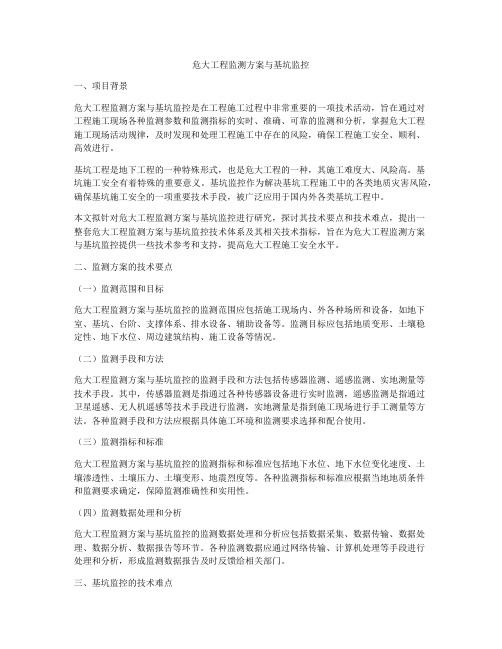
在基坑一端找到稳定的基点设站,以周边基坑影响区域以外稳定的某一固定目标(可以是人工制作的觇标、标记或天线、避雷针等)为零方向,测量出零方向与各观测点之间的夹角, 利用不同周期观测的角度差来直接计算各观测点的位移量。
实际上首次观测时设站点与各观测点之间的视线即为各观测点的基准线, 位移量误差是由测角误差和量边误差引起的。
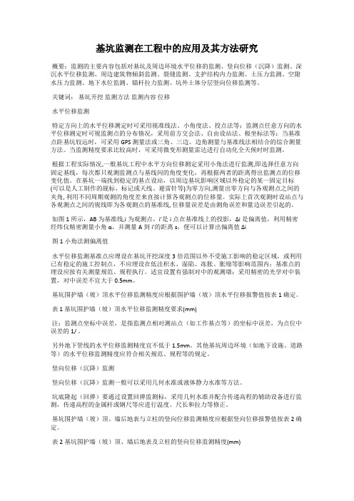
如图1所示,AB为基准线,i为观测点,i’是i点在基准线上的投影,Δi是偏离值,利用精密经纬仪精密测量小角α,并测量A到i’的距离s,便可以计算出偏离值Δi图1小角法测偏离值水平位移监测基准点应埋设在基坑开挖深度3倍范围以外不受施工影响的稳定区域,或利用已有稳定的施工控制点,不应埋设在低洼积水、湿陷、冻胀、胀缩等影响范围内;基准点的埋设应按有关测量规范、规程执行。
适宜设置有强制对中的观测墩;采用精密的光学对中装置,对中误差不宜大于0.5mm。
基坑围护墙(坡)顶水平位移监测精度应根据围护墙(坡)顶水平位移报警值按表1确定。
关于基坑监测技术方案的探讨
关于基坑监测技术方案的探讨基坑工程是指在岩土工程中挖掘的深度较大、面积较广的地下开挖工程,通常是为了建设地下车库、地下商场、地下车站等项目。
由于地下环境的复杂性和施工中产生的变形和水压力等作用下,基坑开挖工程容易引起周边建筑物的损坏和影响周围地下水流动的情况,因此基坑开挖过程中的监测技术方案变得至关重要。
一、地测监测为了了解周围建筑物的情况,需要用到地测监测,可以通过测量挖掘形成的沉降量,判断周边建筑物是否有被动损伤的情况,并采取相应的措施进行修复。
同时还可以通过对地下水的观测记录,实时监测地下水位的变化和水文波动情况,有效控制地下水位,预防因水位变化而引起的灾害事故。
二、变形监测变形监测是指对基坑开挖过程中周围土体的变形的观测、记录分析。
其监测基本要求为高精度、连续性以及实时性,预测基坑开挖过程中可能出现的变形趋势。
其监测方法主要包括传统的钢筋混凝土架式与无线监测技术。
较为常用的监测方法为激光测距方法,通过精确监测土体变形,及时调整土体外部支护结构做出有效的补救措施。
三、水位监测水位监测是针对基坑开挖过程中可能出现的不稳定地下水情况,进行及时有效的监测处理。
水位监测可通过监测仪器对水位进行多点的精度观测,定时进行数据的录取和分析,掌握地下水的变动情况,及时采取措施,以确保其不会对周边建筑物和施工过程造成不良影响。
四、应力监测应力监测是指在基坑开挖过程中,多点应力的智能化观测系统,可通过在线化观测提供土体水准穴位所发生的应力与变形进行实时监测。
其意义在于对基坑周围岩土地质力学特性、土壤的支承力、荷载分布等进行全方位的分析与监测,推算基坑开挖前后岩土较为明显的变化趋势。
综上所述,基坑监测技术方案可综合运用地测监测、变形监测、水位监测和应力监测等多种监测方法。
合理选用合适的检测方法,并通过科学合理的数据分析,能够及时地预警发生可能引起周围建筑物影响、影响地下水流动的风险情况,及时采取有效的防护措施。
关于基坑监测技术方案的探讨
关于基坑监测技术方案的探讨基坑工程指建筑物地下部分的施工,其施工会对周边土体结构产生影响,甚至引发地质灾害,如塌陷、滑坡等。
为了保证基坑施工的顺利进行,并减少对周边环境的影响,需要采取有效的监测技术方案。
一、基坑监测技术的重要性基坑监测技术可以监测施工过程中的土体变形、沉降、荷载变化等情况,及时发现不良变化,防止地面坍塌、裂缝、结构倒塌等情况的发生,早期发现微小的变化,有利于采取及时的应对措施,保障基坑的安全施工。
1. 微震监测技术微震监测技术是一种基于土壤动力学原理设计的非破坏性监测方法,它主要通过监测地下水位变化、土体压力变化、土体位移等变化来实现岩土工程的监测。
通过这种监测手段,可以确保基坑的稳定,同时能够通过对地下水位变化的监测,快速判断出可能涉及到的裂隙或岩石的裂纹情况。
应变计监测技术主要是通过安置应变计在基坑周围以及基坑内部,对土体的变形进行监测。
应变计利用变形后电阻率的变化,对土体进行变形监测,能够反映土体内部的变形情况,判断基坑施工的安全。
3. 钢管桩荷载监测技术钢管桩荷载监测技术,其原理是通过对钢管桩所承受的荷载变化进行监测,可以判断出土体的变形情况。
该技术通过监测基坑周围的钢管桩荷载变化,判断是否出现了地面坍塌、土体滑移等情况。
基坑监测技术方案的选择,需要根据实际情况进行判断,主要考虑以下几点:1. 施工地质条件的不同,需要选择不同的监测手段。
如基坑的地下水丰富,可以选择微震监测技术;如果基坑周围是属于多层地下水的区域,则需要采用应变计监测技术。
2. 监测方法的选择需要参考监测对象的高度和深度,基坑内部和周围的钢管桩以及土壤的生物和化学特性等等;3. 注重监测结果的分析和数据处理。
需要绑定局部和全局稳定性的各种数据来源,较好地进行数据处理、分析和处理;4. 防护与保障要足够。
由于基岩工程施工比较复杂且具有难度,同时也相当危险。
因此,在监测方案的选择时应当做好防护与保障措施,确保施工现场的安全。
基坑监测系统(外文文献) (9)

GEOPHYSICS,VOL.65,NO.1(JANUARY-FEBRUARY 2000);P .83–94,11FIGS.Electrical imaging of engineered hydraulic barriersWilliam Daily ∗and Abelardo L.Ramirez ∗ABSTRACTElectrical resistance tomography (ERT)was used to image the full-scale test emplacement of a thin-wall grout barrier installed by high-pressure jetting and a thick-wall polymer barrier installed by low-pressure permeation in-jection.Both case studies compared images of electrical resistivity before and after barrier installation.Barrier materials were imaged as anomalies which were more electrically conducting than the native sandy soils at the test sites.Although the spatial resolution of the ERT was insufficient to resolve flaws smaller than a reconstruction voxel (50cm on a side),the images did show the spatial extent of the barrier materials and therefore the general shape of the structures.To verify barrier performance,ERT was also used to monitor a flood test of a thin-wall grout barrier.Electrical resistivity changes were imaged as a saltwater tracer moved through the barrier at loca-tions which were later found to be defects in a wall or the joining of two walls.INTRODUCTIONThe cost for remediation of contaminated soil and ground-water at U.S.Department of Defense facilities has been esti-mated to exceed $200billion.Because more than 10000in-dividual sites are involved,each presenting a unique technical complexity,the entire task has become overwhelming.To mar-shal the resources of technology for the task,the ern-ment has attempted to develop new and innovative technolo-gies to reduce clean-up costs while protecting human health.One such technology is subsurface hydraulic barriers,which could be used to completely contain or slow the spread of a con-taminant.A successful barrier might contain the contaminant until natural degradation ran its course,confine the contami-nant during some active remediation,or simply buy time for a site owner.However,for a barrier to succeed it must be easily constructed and cost effective as well as meet certain techni-cal performance criteria.To this end the U.S.Department of Energy has initiated a series of field tests for different barrierManuscript received by the Editor June 22,1998;revised manuscript received January 18,1999.∗Lawrence Livermore National Laboratory,MS L-130,Livermore,California 94550.E-mail:daily1@;ramirez3@.c 2000Society of Exploration Geophysicists.All rights reserved.types at selected but geologically realistic sites.An important element of this program is to determine what methods might be useful to monitor the emplacement and verify the perfor-mance of these barriers without compromising their integrity (i.e.,nondestructively).The most general performance goal for a barrier is to stop or modify in some desired way the movement of a contaminant plume.This means that the emplaced material must modify the in-situ hydraulic conductivity and be continuous (free of holes).In addition,a man-made barrier may be required to meet other criteria,e.g.,seal to a natural barrier such as an aquitard.Evaluating performance can be difficult.A key performance goal is to place the barrier materials in the desired configura-tion.For example,it may be very important to know the path-way and fate of emplaced barrier materials so that the barrier shape,location,and continuity are known.This type of infor-mation could be particularly useful if available in real time to guide construction or suggest any corrective action that might be required before a contractor leaves a site.An ideal technique for monitoring the emplacement and ver-ifying the performance of a barrier requires measurements only from the surface.It would provide a real-time,3-D image of the barrier with resolution capable of detecting even the small-est of defects.Until this ideal is realized,less-than-ideal but currently available technologies have been evaluated:cross-hole radar,electrical resistance tomography (ERT),borehole induction logging,and gaseous tracers.This paper reports the test results from one of these technologies:ERT.ELECTRICAL RESISTANCE TOMOGRAPHYERT is a technique for imaging the subsurface electrical structure using conduction currents.ERT was proposed inde-pendently twenty years ago by Henderson and Webster (1978)as a medical imaging modality and by Lytle and Dines (1978)as a geophysical imaging tool.Early development in geophysics was confined to imaging rock core samples in the laboratory (Daily et al.,1987),but prototype data collection hardware and research-grade in-verse codes suitable for field-scale applications soon followed (Ramirez et al.,1993).More recently,ERT has been developed8384Daily and Ramirezto detect leaks from large storage tanks(Ramirez et al.,1996), to monitor underground air sparging(LaBrecque et al.,1996b), and to map movement of contaminant plumes(Daily et al., 1998).During this entire period,data acquisition hardware and inversion algorithms have been improving rapidly to han-dle the new challenges.Useful evaluation of a subsurface barrier requires more than a series of selected2-D slices;rather,it requires a full3-D rendering of the structure.More recently,fully3-D algorithms have become available.One purpose of this demonstration is to test one of these inversion codes(LaBrecque et al.,1999) under realisticfield conditions.The ERT algorithm we used is based on an Occams-type in-version that yields a minimum roughness solution consistent with the data and their errors.The2-D algorithm,based on a finite-element forward solver,is described by LaBrecque et al. (1996a).Also discussed are mesh requirements used for both the2-D and3-D algorithms.A simple generalization of this ap-proach to three dimensions is impractical,being computation-ally inefficient.However,LaBrecque et al.(1998),describe a method for streamlining the forward solver using an iterative finite-difference formulation which makes3-D inversion prac-tical.Convergence for both algorithms is defined when the rms error,normalized by the weights,is equal to the number of data points.BACKGROUNDTwo different types of barriers were studied using ERT.We first discuss a thin diaphragm wall emplaced by high-pressure jetting of cementatious grout.This barrier was demonstrated at the Groundwater Remediation Field Laboratory located at Dover Air Force Base in Dover,Delaware.The second type was a thick wall emplaced by low-pressure injection of a vis-cous liquid of colloidal silica.This barrier was demonstrated at Brookhaven National Laboratory,Long Island,New York. Both were full-scale demonstrations conducted at clean(un-contaminated)sites.The strategy is to image the subsurface before and after the barrier emplacement so that,by comparing the two images,it is possible to remove the native heterogeneity and highlight only the disturbance from emplaced materials.As it turned out, both sites were quite resistive and the materials for both barri-ers relatively conductive.The resulting high-contrast conduct-ing anomalies were,for the most part,good electrical targets for imaging.In fact,the viscous liquid barrier was so electrically conducting that it could be imaged without the need to remove native heterogeneity in the electrical resistivity structure. Another test involvedflooding a hydraulically enclosed box formed by barrier walls.The strategy was to image the struc-ture before and after the chamber wasfilled with water and to compare the images.From such a comparison,it is possible to remove the barrier itself from the image,leaving only the disturbance from the water tracer and thereby determining the hydraulic integrity of the structure.THIN DIAPHRAGM WALL BARRIERThe test site is underlain by sediments generally composed of medium tofine sands with gravelly sand,silt,and clay lenses. Discontinuous clay lenses are common,and there are occa-sional gravelly sand lenses.Underlying these sands is the20-to28-ft-thick Calvert Formation,which generally consists of gray,firm,dense marine clays with thin laminations of silt and fine sand.Included in the Calvert Formation is the Frederica aquifer,approximately22to28m below ground surface.De-tails of this geology can be found in Pellerin(1997a). Borehole induction logs and core sample measurements showed that the electrical resistivity of the sands varied be-tween300and600ohm-m while that of the clay was less than 50ohm-m.Resistivity of the grout varied widely,depending on the exact formulation and the curing boratory mea-surements place the electrical conductivity for the formulation between10and30ohm-m(Pellerin,1997a).There is good electrical contrast between the grout and the native sands.On the other hand,contrast may be low with the clay-rich soils that form the bottom of the barrier.Vertical grout panels were placed into the sands in vari-ous configurations with the goal of constructing a hydrauli-cally closed container.Each panel was formed by a high-velocity grout stream jetted horizontally from a lance as it was slowly withdrawn from the subsurface.The high-velocityfluid, a grout–bentonite mix,eroded a cavity deep into the soil.The resulting panels were placed so they overlapped along their sides to seal together and so they penetrated the clay acquitard (Calvert Formation)along their bottoms.(The clay provided the bottom to the box.)The entire structure was to become a hydraulically sealed box.Results of the technique are shown in Figure1,which is an excavation of the end of a test box formed by three intersecting panels.Notice the columnar structure near the center of the end panel.This is a cast of the grout-filled injection hole.Thefigure illustrates the wall thickness and how panels overlap at the edges to ensure a hydraulic seal.The plan was to emplace two concentric cylindrical walls in the sands,keying them along the bottom into the clays.The plan was later changed,after the boreholes used for ERT were installed,so that only the interior wall was emplaced.Figure2 is a plan view of the site,including the ERT boreholes and how the grout panels were tofit together.Each of the ERT electrode arrays indicated in Figure2con-tained15electrodes evenly spaced between the surface and 15m depth.Electrodes were fastened onto the outside of a PVC casing,and the borehole was completed with a sand backfill. This arrangement made it possible to use the holes for other geophysical or hydraulicmeasurements.F IG.1.Excavation of a thin diaphragm wall test barrier at theDover test site.ERT of hydraulic barriers 85The reconstruction mesh contained 144000voxels although only 48000(each approximately a 1-m cube)defined the image;the others were used to properly model the boundaries.A total of 6480transfer resistance measurements were used for the re-constructions (12960if reciprocal measurements are counted).The number of parameters to be determined (144000)is much larger than the number of linearly independent data (6480),so the problem appears grossly underdetermined.Fortunately,because a solution of minimum roughness is calculated,each voxel is not an independent unknown but depends on the val-ues of nearby voxels (see LaBracque et al.,1996a).Preemplacement and postemplacement data were collected on the 16hole pairs shown in Figure 2to densely sample the image volume within the borehole ring.On October 3,1997,a total of 12960transfer resistances were measured for the baseline,half of these being reciprocal measurements used to estimate data accuracy (LaBrecque et al.,1996a).About 10hours were required to collect the data.The barrier wall was then installed in November,and ERT surveys were repeated between December 3and 4.Thin diaphragm wall resultsFigure 3shows the 3-D ERT images of a thin diaphragm wall barrier at the Dover test site.Figures 3a and 3b are the baseline image block before installation.The sands above about 10.7m depth have a conductivity of 10−5to 10−6mS/m and comprise most of the block.Figure 3b shows only the clay basement (conductivity >10−5mS/m).The barrier panels are to be keyed into this surface.The goal is to achieve a hydraulic seal between the clay and the walls,so the reader will want to pay special atten-tion to this part of the ERT image.The panel walls were installed to approximate a cylinder 10.6m in diameter.Figure 3c is a voxel-by-voxel difference in conductivity between the baseline and data collected on December 4,1997.The image is rendered transparentwhereF IG .2.Plan view of the thin diaphragm wall panel arrange-ment to create a large,hydraulically enclosed box,the bottom of which is a clay-rich aquitard at 10.5m depth.There are nine ERT electrode arrays (and twelve holes used for other geo-physics),each with fifteen electrodes evenly spaced between 1and 15m depth.The dashed lines indicate the hole pairs used to acquire ERT data for the 3-D reconstruction block,which is 21.3m square and 14m deep.the conductivity change is <3×10⁻⁶mS/m.This threshold is arbitrary.A very much lower value produced several anoma-lies that we judged as measurement errors propagating through the algorithm.A very much higher value can make the barrier anomaly become arbitrarily thin.We believe this threshold value best represents the experimentally significant changes in the subsurface.Because several things changed the subsurface conductivity during this period,other anomalies obscured the clear view of the barrier.These anomalies are discussed later.However,if we temporarily remove these features,the barrier becomes clear (Figure 3d).A quadrant of the barrier anomaly is re-moved to show features inside more clearly.From this last part it appears that the barrier structure is approximately as planned:a continuous cylinder extending from the clay–sand boundary to near the surface.Notice also that the wall thickness appears to be about 1.5m near the center but tapers toward the top and bottom edges.The exaggerated wall thickness as well as the tapering are both likely an artifact of the way the inversion algorithm searches for a smoothest solution.While Figure 3provides a good perspective view of the grout emplacement,some of the significant details are difficult to see.Figure 4shows,in plan view,a series of horizontal sections through the image volume.From these sections it is easier to see details.Starting near the bottom at 13m depth (Figure 4a),we see the anomalies associated with each ERT borehole.(These anomalies were removed from Figure 3d.)Because the other geophysical wells do not show such anomalies,we believe these conductive anomalies result from small amounts of salt water poured down the annulus of each ERT well to lower the con-tact resistance at the electrodes because of the dry sand backfill.Apparently,the salt water—all of which was not retained in the sand column by capillarity—drained to the hole bottom and in time found its way into the formation.The disturbance was confined to the bottom of each hole because only 8or 9liters of water were used for each electrode array.Above 10.5m depth (Figure 4b),these anomalies are nearly absent.The deepest evidence of the barrier in the image is shown in Figure 4b at 10.5m.A section near the middle of the image block at 7.5m is shown in Figure 4c.ERT does not show the barrier shallower than 3.7m (Figure 4d);however,between 10.5and 3.7m there is a continuous,circular anomaly repre-senting the barrier.Before discussing the shallow section at 0.76m in Figure 4e,we will consider details of Figures 4a–4d.Grout injection to form each panel was between 13m (Figure 4a)and the surface,yet the ERT image extends from 10.5to 3.7m depth.We are not certain why the barrier anomaly does not extend over the full range,but two possibilities have been considered.First,the sensitivity of the ERT algorithm is lower at both the top and bottom of the image block because there is less data coverage there relative to the center of the image block.It is possible that the thin wall cannot be resolved with this reduced sensitivity.A more likely explanation for the lack of sensitivity at the bottom is the presence of the boratory measure-ments of grout conductivity depended on exact formulation and curing time but ranged between 10and 40ohm-m (Pellerin,1997a).The Calvert Formation (the clay)is between 10and86Daily and Ramirez100ohm-m and may offer insufficient electrical contrast for the grout.One or both of these facts may explain why the barrier was not imaged as deep or as shallow as expected.Notice that the image shows no gap or flaw in the barrier anomaly where it intersects the clay at about 10.5m depth.We believe that the ERT data are consistent with continuous grout panels as deep as 13m but were not imaged that deep because of low electrical contrast with the clays.In the 7.5-m section the barrier is a smooth (Figure 4c),con-tinuous circular anomaly.Resolution is insufficient to distin-guish individual panels.Also notice that the barrier image is 9m in diameter,while injection was 10.6m in diameter.We do not know the reason for this difference.Examination of sections shallower than 3m reveals a se-ries of conductive anomalies as shown in Figure 4e.(These F IG .3.A thin diaphragm wall barrier at the Dover test site shown in Figure 2.(a)The 3-D image block of electrical conductivity before barrier emplacement (the baseline).(b)The baseline 3-D image block,showing only the formation >10−5mS/m electrical conductivity.This is the clay aquitard at 10.5m which forms the bottom of the enclosed barrier.(c)A voxel-by-voxel difference between the baseline and postemplacement image block.Only changes in electrical conductivity from 3×10⁻⁶and 2×10⁻⁵mS/m are shown.(d)Same as (c)but with all borehole and surface anomalies removed.Only the barrier remains,with a quadrant removed to make the inside visible.were also removed from Figure 3d.)They roughly define the circumference of a 15.2-m-diameter circle centered on the site.Prior to barrier installation,an asphalt base (called a mud mat),15.2m in diameter,was installed to catch any grout spill at the surface during the high-pressure injection.These anomalies are likely the result of small quantities of grout that spilled off the edge of the mud mat and washed into the surface soils.Detecting these anomalies in a region of the image block of reduced sensitivity is evidence that we should have imaged the grout wall above 3.7m depth if it were present.We conclude from the results that ERT provided an image of the thin-wall grout barrier even though some details of the images do not match our expectations of the structure (e.g.,anomaly diameter slightly different from the circle defining the injection locations).ERT of hydraulic barriers 87The image is consistent with a thin wall (i.e.,40cm,typical of other thin diaphragm walls that had been excavated)and is uniform from top to bottom.There is little evidence from this image of grout material being spread much beyond the intended wall configuration.Spatial resolution in these images was about 1m;therefore,details in the wall structure are not visible.Small holes or gaps at the intersection of two walls may not be resolved.If we assume that grout,unsuccessfully injected into the clay,would end up in the more permeable sands,then the undistorted interface of the panel at the sand–clay boundary is consistent with panels successfully keyed into the clay acquitard.The upper and lower extremes of the panels are not imaged by ERT.The lower parts were likely not imaged because of the low electrical contrast with the clay-rich sands below about 10.5m.We do not know why the panels are not imaged above 3m.F IG .4.The same thin diaphragm wall barrier shown in Figure 3but in plan view,with the conductivity differences of the image block sectioned at various depths.(a)The horizontal section at 13m,which is 2.5m into the clay.This is the bottom of the injection interval for the panels.The conductive anomalies correspond to the ERT borehole locations.(b)The horizontal section at 10.5m,which is the lower boundary of the barrier image and the upper bound of the clay layer.(c)The section at 7.5m,the image block center,showing the conductive anomaly of the barrier and a superimposed circle of 10.6m,which is the injection circle.(d)The section at 3.7m,which is the upper bound of the barrier anomaly.(e)The section at 0.76m.A circle of 15.2m is superimposed to show the size of the mud mat.THIN DIAPHRAGM WALL BARRIERVERIFICATION—FLOOD TESTERT was used to image tests on another barrier formed with the high-pressure,thin-diaphragm-wall technique at the same Dover test site described in the previous study.The box has a bottom formed by the clay aquitard at about 3.8m depth with thin-wall grout sides and is open at the top.Salt water was used as an electrical tracer to determine the presence and location of any leakage flow paths.Figure 5illustrates the configuration for the walls of this box.After the barrier was installed,a series of ERT electrode ar-rays was installed,each of 7electrodes equally spaced between the surface and 6m yout of the arrays is shown in Figure 5.The reconstruction mesh consisted of 21600voxels.Only 1400of those are shown in the image volume;the rest are used to model the boundaries.A total of 1078transfer88Daily and Ramirezresistance measurements were used for the reconstructions (2156if reciprocal measurements are counted).On August18,1997,a total of2156baseline transfer resis-tances were measured from the14hole pairs shown in Figure5. Then on August19at1100hours,saltwater tracer was added to the box through a screened water monitoring well near the center of the box.Sodium chloride was added to the native groundwater,with conductivity of1.5×10−4S/cm to raise it to4.3×10−3S/cm.This water was released into the box at 7.6liters/min.Three-dimensional ERT data sets were taken during theflood on August19and again on August20after theflood ended.The goal was to observe the water tracer by comparing the baseline and subsequent images.Results of thin diaphragm wall boxflood testFigure6shows the changes in resistivity of the image block as a result offilling this small,nearly rectangular box.The box walls and clay base are absent from the image since they are in both the pre-and postflood data.We made the image block transparent except where the de-crease in resistivity was30%(early in theflood)or35%(later in theflood or after theflood).In each case,this isocontour was then sectioned at11equally spaced intervals between the surface and6m depth.This rendering allowed us to view all sides of the tracer plume at each snapshot in time:1130to 1346hours on August19after about456liters of tracerwaterF IG.5.Plan view of the thin diaphragm wall panel arrangement to create a small,hydraulically enclosed box,the bottom of which is a clay-rich aquitard at3.8m depth.There are eight ERT electrode arrays,each with electrodes evenly spaced from the surface to6m depth.The injection borehole was a screened water-monitoring well.was added;1418to1620hours on August19after about1824 liters was added;and0703to1046hours on August20,which was about17hours after theflood ended.This format gives a good overall view of the plume as it is forming inside the barrier.In thefirst image the plume extends directly below the release point,but only to a depth of about 4.2m.By day’s end on August19,the plume has grown verti-cally to almost6m depth and is also much wider.There is no evidence at this high infiltration rate of the barrierfilling from the bottom up like a bathtub.On August20,approximately 17hours after infiltration ended,the plume is spreading hor-izontally to the left in thefigure.To better see the implica-tion of this,Figure7plots each of the plume sections in plan view.Figure7shows each of the plume sections for the early to-mograph(1130to1346hours)from0.6to5.4m depth.The iso-surface is relatively compact and is centered on the infiltration point.The connection with the surface is missing because the infiltration well was not screened all the way to the surface.The plume extends only to4.2m depth.The clay aquitard,which starts between3.8and4.0m,is likely impeding the downward migration of the plume so that it is not imaged below4.2m. This view of the plume also shows an interesting hydraulic pathway difficult to observe in situ:the plume below3.0m ap-pears nearly disconnected from the plume above1.8m.There is only a narrowflow path connecting the two,shown here by the small isocontour at2.4m.This feature probably results from natural and subtle heterogeneity in the sands.However, we will see that its effect disappears in later images.By the end of theflood,Figure8has the plume extending all the way to5.4m depth,and it has also grown laterally. These images are still consistent with the plume being com-pletely contained by the grout walls,even though the contours extend a little past the barrier outline.(The images are spa-tially smoothed,so the lateral extent is probably exaggerated.) The plume extends about1.6m into the clay aquitard,which starts at about3.8m.Figure9shows a different behavior.While the plume has not changed significantly in the top or bottom sections,between2.4 and4.2m depth the contour extends significantly beyond the left panel.Even at1.8m depth,the contour points suspiciously to where two panels join at the top-left corner in thefigure.We interpret this as a leak in the left wall or at the junction between the left and upper wall.The breach appears to be between1.8 and4.2m depth.This barrier was excavated after the test, and the walls were examined.The two panels did not join completely in the upper-left corner at a depth of about3m. The excavation results are consistent with the depth range of the tracer leakage as observed in the images.VISCOUS LIQUID BARRIERThe test site at Brookhaven National Laboratory,located on Long Island,New York,consisted of unconsolidated glacial deposited sediments primarily composed offine-to coarse-grained quartz sand with some gravel.Groundwater was about 13m below grade(at the base of the ERT image plane).De-tails of this geology and the site characterization are found in Pellerin(1997b).Electrical resistivity of the sands varied between300and 1000ohm-m.Resistivity of the neat colloidal silica(the viscousERT of hydraulic barriers 89liquid)varied,depending on the exact formulation and the curing time.Pellerin (1997b)reports laboratory measurements on the order of 1ohm-m for cured material so the emplaced barrier will produce a strong conductive anomaly relative to the native soils.The plan was to emplace two parallel vertical walls and one sloping wall between them to provide three sides and the bot-tom of the containment structure.A fourth wall (vertical)com-pleted the enclosure.Figure 10illustrates the arrangement (see Pellerin,1997b).Each wall is actually three rows of cylinder-like structures fused together.Each cylinder was formed as the polymer was injected under low pressure from the end of a lance (permeation of the material into the soil),slowly with-drawn from the soil.The primary row of grout cylinders was formed;then a secondary row was placed about 75cm from the first;and then the final row was emplaced about 75cm from the second row.Although the viscous liquid barrier imaged in this test was excavated,photographs of the structure are of little use since the colloidal silica is transparent and the structure is not self-standing as in the case of the diaphragm wall.Definition of the wall structure was only possible by measuring electrical conductance of the soil as it was excavated.Therefore,we F IG .6.The 3-D image block,showing the ERT changes in resistivity from baseline during and after the flood test.The fi-nite-difference mesh and the approximate outline of the barrier walls are projected onto the top surface.The ERT boreholes are also shown.(a)The saltwater tracer plume imaged early in the flood between 1130and 1346hours on August 17.Resistivity changes of 30%are shown.(b)The plume imaged at the end of the flood between 1418and 1620hours.Resistivity changes of 35%are shown.(c)The plume imaged on the day after the flood test.Resistivity changes of 35%are shown.have no excavation photographs of the viscous liquid barrier walls.However,we do have other information collected during excavation to compare with the ERT images.The ERT electrode array 5in Figure 10contained 15elec-trodes evenly spaced between 1m and 15m depth.Arrays 1and 4were shorter and had fewer electrodes so as not to inter-cept the barrier once it was emplaced.The strategy with this arrangement of ERT electrodes was to produce a 2-D image of the section defined by the boreholes.The reconstruction mesh contained 15202-D pixels,although only 560define the image;the others are used to properly model the boundaries.A to-tal of 274transfer resistance measurements were used for the reconstructions (548if reciprocal measurements are counted).Before emplacement of any barrier material,baseline ERT data were taken on June 19,1997,between borehole pairs 1,4,and 4,5.The primary or first row of injectate for the slant wall was completed during the last week of July,and on July 31another ERT data set was collected.The remainder of the barrier walls were installed,and on September 19ERT data were collected again.These data allowed for a comparison of the slant-wall images after one row of injectate and with all three rows.Notice that the side walls,already in place dur-ing the September 19data,present high contrast features that。
基坑监测系统(外文文献) (8)

GEOPHYSICS, VOL. 60, NO. 3 (MAY-JUNE 1995); P. 886-898, 15 FIGS.Cross-borehole resistivity tomography of a pilot-scale, in-situ vitrification testB. R. Spies* and Robert G.ABSTRACTDirect current (dc) cross-borehole resistivity mea-surements were used to monitor the melting andsolidification processes of an in-situ vitrification (ISV) experiment at Oak Ridge National Laboratory (ORNL) in Tennessee. Six boreholes, 6-m deep, were augured around the ISV site, and five electrodes implanted in each hole. Three sets of crosswell, pole-pole resistivity data were collected: prior to the melt phase, immediately after power shut-off, and after themelt zone had solidified and returned to ambienttemperature. These three sets of data were invertedusing a conjugate-gradient scheme to produce conduc-tivity images of the melt phase and the vitrified endproducts.The images obtained depend quite strongly on themodel weighting function applied to the inversion.With an optimum weighting function based on a priorispatial constraints, the resistivity images delineate themelt zone and provide a reasonable indication of itsgeometry. The resistivity data support, but do notrequire, the existence of the melt zone.INTRODUCTIONIndustrialized nations are faced with increasing amounts of toxic and nuclear waste arising from commercial and military development. The U.S. Department of Energy (DOE) is funding various research efforts aimed at evaluat-ing safe remedial alternatives. Of particular interest are techniques for containment of radioactive waste buried in pits and trenches during the past 40 years as a byproduct of the U.S. government’s domestic energy and military pro-gram. The high radioactivity of these materials precludes excavation, which could potentially release contaminants into the air and endanger personnel.In-situ vitrification (ISV) is one possible remedial technol-ogy that could be applied to wastes in pits and trenches; others include grouting and ground densification. The ISV process, developed by the Pacific Northwest Laboratory (PNL) for DOE, involves placing electrodes in and around the contaminated volume of soil, applying power to the electrodes, and melting the entire mass of soil into a chem-ically homogeneous and durable glassy-to-microcrystalline waste form that is resistant to leaching (Spalding et al., 1992). ,Unfortunately, it is difficult to predict the progress of the melt process. Power must be applied long enough for the melt to encompass all the waste material. The melt temper-ature should be high enough for the melt volume to expand at a reasonable rate, yet low enough to minimize radionu-clide volativity. A remote sensing technique, capable of monitoring the extent of the melt, is therefore highly desir-able.For the pilot-scale study described in this report, direct monitoring of the melt was accomplished by the use of 93 thermocouples and optical pyrometers. in vertical arrays installed during construction of the trench. Thus, the progress and temperature of the melt could be accurately determined. However, during application to an actual waste site, this method of depth monitoring is not feasible because sensors cannot be emplaced in a contaminated site. Other methods, such as monitoring energy usage and performing heat flow calculations, are less desirable than direct moni-toring via geophysical methods.Geophysicists at the University of Tennessee planned to use surface and crosswell seismic techniques to monitor the melt process (Jacobs et al., 1992). In conjunction with the 2-D seismic experiment, we proposed to conduct a low-cost 3-D crosswell dc resistivity survey using off-the-shelf equip-ment borrowed from the University of Tennessee. The resistivity survey was designed to demonstrate what couldPresented at 63rd Annual Meeting, Society of Exploration Geophysicists. Manuscript received by the Editor November 10, 1993; revised manuscript received September 2, 1994.*Schlumberger-Doll Research, Old Quarry Road, Ridgefield, CT 06877-4108.of Geophysics and Astronomy, University of British Columbia, Vancouver, Canada V6T 124.© 1995 Society of Exploration Geophysicists. All rights reserved.886Cross-borehole Resistivity Tomography887be accomplished with inexpensive off-the-shelf resistivity equipment in a short time frame and with low budget, and toassess the applicability of borehole electrical tomography in imaging the ISV process. The electrical resistivity imagingexperiment described in this paper was designed and imple-mented in less than three weeks, a strict timetable dictatedby the imminent ISV pilot.The Pilot-Scale ISV TestA series of seven seepage pits and trenches were used between 1951 and 1966 at Oak Ridge National Laboratory (ORNL) for the disposal of approximately 1.6 x 10⁸ 1(4.3 x10⁷ gal) of liquid waste containing I million curies of radioactive material. Figure 1 shows the design of a typical seepage trench. These trenches were located on the peaks ofridges to facilitate seepage of liquids, and filled with crushedlimestone or dolomite. As liquids seeped out, the 137Cs and 90Sr remained in, or in close proximity to, the trenches (cesium is sorbed by the illite-rich soil, and strontium wasmade less mobile by treatment with a highly alkaline solution at the time of disposal). The pits and trenches are now covered with asphalt caps to reduce the flow of precipitation through the waste.ISV is a relatively recent candidate technology for in-situ remedial treatment of waste (Oma et al., 1982). ORNL and Pacific Northwest Laboratories (PNL) conducted a series of pilot-scale “cold” (no radioactive components) ISV tests in 1987 to begin evaluation of the technology. A conceptual sketch of the ISV operating sequence is shown in Figure 2. Gases and particulates produced during the high temperature (1300 to 2000°C) operation are diverted by a hood under aF IG. 1. Design of a typical seepage trench used from 1951-1966 at ORNL. The trench was filled with crushed limestone or dolomite to facilitate seepage. Radionuclides were in-tended to remain within or close to the trenches as liquids seeped out (from Spalding et al., 1992).slight vacuum to an off-gas treatment system that scrubs and collects contaminants released into the off-gas.The 1991 pilot-scale ISV experiment at Oak Ridge was the first to use small, precisely known amounts of radioactive material (mostly 137Cs and 90Sr). The experiment was con-ducted at one-half scale of a typical ORNL trench. To permit emplacement of the temperature sensors, a large excavation, 13.5 m square at the surface and 5.5 m square at a depth of4.3 m, was dug and then backfilled with the sensors in place.A half-scale seepage trench was constructed inside the larger excavation, and a small quantity of radioactive waste sealed in plastic bottles was placed near the bottom of the limestone layer.ISV Pilot-Scale ResultsA photograph of the ISV test site prior to melting is shown in Figure 3. Approximately 28 MW.h of cumulative power was applied to the melt over a five-day period at an average power level of 220 kW. Power was turned off intermittently for seismic measurements and equipment problems. The operating temperature of the melt was approximately 1500°C. At this temperature the viscosity is 100 poise, and convection is the dominant heat transfer process within the melt (Spalding et al., 1992).Accurate estimates of the shape of the melt during the experiment were obtained from the temperature data. Tem-perature gradients within the melt are small, usually less than 100°C over the volume of the melt. However, temper-ature gradients across the melt-soil interface are high; tem-peratures dropped from over 1000°C to 100°C over a distance of only 1 m from the melt-soil contact. A narrow low-pressure (P888Spies and Ellisthe temperature remained at 1145°C for 20 hours as a result of latent heat of crystallization released as the molten product precipitated mineral phases.After several months, the body cooled to near-ambient temperature and drill cores were taken to determine its shape and obtain samples. The final shape was an elongate hemisphere with the central portion 2.6 m deep and the margins 2.1 m deep (Figure 4). The upper surface of the melt subsided 1.5 m below ground surface because of volume reduction during melting of the soil. The solidified product was almost entirely crystalline, although the material around the perimeter was somewhat glassy.Thermal Effects on ResistivityMolten rock is highly conductive. Typical values for basalt, andesite, and obsidian are 3 to 10 S/m at 15OO°C, decreasing to 0.2 to 1 S/m at 1000°C (Murase and McBirney, 1973). Laboratory measurements of electrical conductivity of various mixtures of soil and limestone representative of the pits at the ORNL site are described by Shade and Piepel (1990). Electrical conductivity was measured at the temper-ature at which 100-poise viscosity was achieved: for pure soil the conductivity was 2.8 S/m at 1735°C and for a 50% soil - 35% CaO - 15% Na20 mixture, the conductivity was 11 S/m at 1200°C. The highest conductivity obtained (for a 67% soil composition) was 26 S/m at 1233°C.F IG. 3. Photograph of ISV test site prior to melting. Power is fed to the melt via the four protruding graphite electrodes. Gas and particulates are collected in the off-gas hood and scrubbed to remove contaminants. Six 6-m deep boreholes, each with five electrodes and located in a 12-m diameter circle around the hood, were used for the crosswell resistiv-ity experiment. Progress of the melt was monitored by the use of 93 thermocouples and optical pyrometers placed in vertical arrays during construction of the waste trench (from Jacobs et al., 1992).Initially we assumed that the ISV melt would be a con-ductive target in relation to the background soil and based the presurvey modeling on this supposition. However, more detailed analysis of the thermal and hydraulic regime sur-rounding the melt reveals that the resistivity structure is likely to be much more complex than first supposed. Consider a temperature profile starting at background values (20°C) and moving toward the melt. Initially the resistivities will be typical of the clayey soil in the area, around 200 ohm-m. Contributing to the electrical conductiv-ity of the soil is ionic conduction in the pore water and exchangeable ions on the surface of clay particles. The soil at ORNL is approximately 50% porosity with a water content of roughly 20 wt%. The salinity of the pore waters is low, with an ionic strength of 5 x 10⁻⁴ to 10-3 normality, and a resistivity of around 200 ohm-m. A rough composition of the soil is: illite (40 wt%), vermiculite (10 wt%), kaolinite (10 wt%), quartz (30 wt%), and carbonates (10 wt%), with a bulk density of 1.35 g/cm3.Clay conduction takes place by ionization of clay minerals and electrolytic conduction through the double layer on the surface of clay particles. Illite and vermiculite provide the main conduction path since they have the highest concentration of counter-ions of the clay minerals present. The bulk resistivity of soil at ORNL (200 ohm-m) is higher than that expected for clay (1 to 5 ohm-m) because the near-surface soils are partly aerated and poorly compacted, and the high rainfall tends to leach the exchange ions from the clay particles (Keller and Frischknecht , 1966).At some location in the melt profile, the temperature of the soil will begin to rise above background values through thermal conduction from the melt. Water conductivity in-creases with temperature according to Arp’s (1953) equa-tion, by about a factor of 3 from 20°C to 100°C. Clay conductivity is governed by the cation exchange capacityF IG. 4. Three-dimensional plan and cross-section of the thermocouple data at the end of the melt stage. The melt body is approximated by the 1000°C isotherm. The final shape of the body obtained from coring is shown as the transparent white solid. The lighter surface represents the 100°C isotherm around the melt. Graphite ISV electrodes are shown as white rods (from Jacobs et al., 1992).Cross-borehole Resistivity Tomography889and mobility of the double layer. Laboratory studies on the temperature dependence of the exchange capacity of clays generally show only a small dependence on temperature, but a large dependence on ionic mobility. Using empirically derived data from Sen and Goode (1992). the ionic mobility, and hence the electrical conductivity of typical clays, should increase by about a factor of 4 from 20°C to 100°C.A counteracting effect on the increase in electrical con-ductivity of clays with temperature is dehydration. Dehydra-tion of clays involves two aspects: removal of bound and interlayer water at relatively low temperatures (typically below 130°C, and often as low as 40°C, depending on confining water pressure), and dehydroxylation (loss of OH in the clay lattice) at much higher temperatures, typically around 300°C (Grim, 1968; Earnest, 1984). Both illite and vermiculite exhibit considerable dehydration at tempera-tures below 100°C (Grim, 1968), starting at about 40°C. The amount of dehydration depends on the initial saturation and the relative humidity of the surroundings. Thus, as temper-ature is increased from 20°C, we may expect an initial increase in conductivity and then a decrease as the clays start to dehydrate and lose their bound and interlayer water.At 100°C the free water in the pores boils off. Some water is drawn in from regions surrounding the melt through capillary action, but at some point all the water will be boiled off and the temperature will rise rapidly. All bound water and interlayer water will be driven off completely between 120°C and 140°C (see, for example, thermogravimetry experiments in Earnest, 1984), and the resistivity of the soil will rise dramatically. As observed in the ISV test (Jacobs et al., 1992), thermal gradients across the melt-soil interface are high: temperatures measured from thermocouple data dropped from above 1000°C to 100°C over a distance of approximately 1 m from the melt-soil contact. Moving im-mediately adjacent to the melt, electrical conductivity would be expected to rise again at the transition zone, where the soil starts to melt (around 900°C), to its highest values in the melt proper at 1500°C.It is now possible to construct a conceptual resistivity profile as shown in Figure 5. The temperature data were gathered from the thermocouple array mentioned earlier. Resistivity decreases somewhat linearly with temperature to between 40°C and 100°C, then rises linearly with a dramatic increase at 120°C. The resistivity will drop steeply at around 900°C as the soil starts to melt.Thus we see that the resistivity section of the melt and surrounding area is likely to be very complex and difficult to image with a remote sensing geophysical technique.CROSSWELL RESISTIVITY SURVEY Survey DesignInitial modeling of the expected difference in response between premelt and postmelt conditions suggested that the change in dc potential in a crosswell tomographic survey would be very small, of the order of several percent. Optimal survey design and data acquisition procedures were there-fore critical.The short time frame and low budget precluded the construction of a sophisticated multichannel system. In-stead, a single-channel Syscal R2 resistivity system was borrowed from the University of Tennessee. The Syscal R2, manufactured by BRGM, has a rated accuracy of 0.3 to 1%, automatic stacking and self-potential bucking, and a maxi-mum output current of 1 A at a power of 700 W.Survey design was hampered by very strict interpretations of environmental regulations by Martin Marietta Energy Systems. Also, because we were working in a DOE facility in the vicinity of both radioactive and hazardous waste, we were urged to avoid creating more mixed waste. These conditions imposed extra limitations, and we were unable to use traditional nonpolarizing lead electrodes or salt water. We used, instead, copper sheeting as electrodes (far from ideal from an electrochemical viewpoint) and distilled water, supple-mented by timely rain showers, to water the electrodes.Six 6-m deep holes were augered at approximately equidis-tant intervals around the ISV site (Figure 6). The holes were located several meters from the vent hood, resulting in a spacing of 5 to 8 m between adjacent holes and 12 m between opposite holes. Five electrodes were placed in each borehole.F IG. 5. Conceptual temperature and resistivity profile through the melt. (a) cross-section showing electrode loca-tions and isotherms during ISV melt process, (b) tempera-ture and resistivity profile. There is a steep thermal gradient across the melt-soil interface, where temperatures drop from >1000°C to 100°C over a distance of 1 m. The conductive melt is encapsulated by a thin dehydrated shell of very high resistivity.Cross-borehole Resistivity Tomography where the first term represents a data misfit measure, and thesecond represents a model structure measure. The datamisfit measure is the sum, over all data, of the differencesbetween the measured and predicted potentials normalizedby the measurement errors. The second term ensures thatthe final model not only fits the data but is simultaneously assmooth as possible. The parameteris a model weighting function. The param-eter is minimized0), or whether ln isa reference or background model. Typical values of(2)that accentuates model variation in the interborehole region.The scale factor 0.1 controls the maximum amount ofdeviation and andin the referencemodel. The reference model892Spies and Ellispremelt data and were inverted to give models with pre-dicted data having 1 to 2% rms misfit.The melt and postmelt images show large conductivityvariations in the vicinity of the boreholes where the sensi-tivity of the dc resistivity technique is highest. This occurseven though we have forced the data to fit the smoothestmodel=3 m) and suppresses structure ( c = 1) within 1 to 2 m of theboreholes =6 m,Cross-borehole Resistivity Tomography893DISCUSSIONWe should emphasize that inversion of any geophysicaldata is a nonunique process; this is particularly true of dcresistivity. Many models fit the data to the same level ofmisfit. From this perspective, the models shown in Figures 7to 13 are representatives only of a class of possible modelsand cannot be considered definitive. Rather, they are possi-ble models of the earth conductivity distribution consistentwith measured data that minimize the objective function.The weighting functions described by equations (2) to (4)are designed to minimize resistivity variation in the vicinityof the boreholes where sensitivity is very high, and favorstructure between the boreholes in the expected region ofthe melt location. We see, though, that the locations of theboundaries of the structure are strongly controlled by theparticular choice of weighting function.We would expect that decreasing the distance between theboreholes, and adding other electrodes on the surface, inextra boreholes, and at greater depths, would improve theresolution of the image, but the placement and total numberof electrodes is always constrained by operational consider-ations. Certainly an automated multichannel acquisition894Spies and Ellissystem would have speeded up data acquisition time and increased data accuracy. The ultimate resolution of any inverse technique is controlled by the sampling aperture and coverage, as well as by the fundamental physics and non-uniqueness of the measurement. Resolution studies on syn-thetic models often fail to take into account realistic varia-tions in resistivity at or near the electrodes, ignore normal geological heterogeneity, and usually underestimate the op-timum number of electrodes required for adequate coverage. The most important task, from the standpoint of the ISV experiment, is to image the base of the ISV melt. Our results suggest that the existence of the ISV melt is not required by the dc resistivity data, but rather, is supported by it. We can enhance the image by a judicious choice of weighting func-tion, but are unable to accurately map the depth extent of the melt body.To better delineate the base of the highly conductive melt zone, it might be preferable to employ an inductive EM technique because induced currents would not be shielded by the resistive shell. A crosswell EM system operating at high frequencies (tens to hundreds of kilohertz) has a nar-rower sensitivity pattern (Spies and Habashy, this issue) than low-frequency EM or dc techniques and would be expected to provide better focusing and resolution.CONCLUSIONSThe 3-D resistivity tomography experiment was successful in imaging the ISV zone in its various phases of premelt,melt, and postmelt. To obtain an optimal image of the melt zone from the inversion it was necessary to apply a weight-ing function that emphasizes structure in the interborehole region and suppresses artifacts caused by high sensitivity near the electrodes.The ISV melting process results in a very complex con-ductivity profile, which includes a highly conductive melt encapsulated by a thin, but highly resistive shell that results from total dehydration of the soil at elevated temperatures. This resistive zone, in turn, is surrounded by a moderately conductive region where the soil is heated to temperatures below 100°C.The resistivity inversion with a narrow weighting function appears to support a two-zoned resistivity model of the melt phase, but this result is probably an artifact of the inversion process. The image changes substantially as the weighting function is varied. The sensitivity of the images to the choice of weighting function results from nonuniqueness and equiv-alence inherent in resistivity inverse problems.The experiment successfully demonstrated that an inex-pensive off-the-shelf resistivity system could be used toF IG. 11. Vertical north-south slices through the approximate center of the melt with the localized weighting function of equation (3): (a) premelt, (b) melt, (c) postmelt.F IG. 12. East-west slices of the melt model obtained with two different weighting functions. The top and center images are inversions obtained with a broad cylindrical weighting func-tion and misfits of 5.0 and 2.8%. The lower image is the same as that shown in Figure 10b (misfit 1.3%). which was obtained with an elliptical weighting function. The image obtained is closely related to the weighting function used.Cross-borehole Resistivity Tomography895F IG. 13. An inversion of synthetic data from a homogeneousearth model with 5% random noise obtained with the ellip-soidal weighting function used in Figure 10. Only minorartifacts are present. The data misfit is 4.8%.acquire high-quality 3-D resistivity shallow borehole datasuitable for tomographic imaging. However, data acquisitionwith the single-channel resistivity system was slow, and anautomated multichannel system would be preferable.The dc resistivity technique is the simplest electricalmethod that can be used for crosswell imaging. However,any dc method is unlikely to directly detect the melt zonebecause the resistive halo acts as an insulating shield tocurrent flow. An inductive electromagnetic technique oper-ated at high frequencies would be more suitable for directdetection of the conductive melt zone.ACKNOWLEDGMENTSWe thank Gary Jacobs and other staff at ORNL for accessto the ISV site and for their encouragement. The pilot-scaleISV test offered a unique opportunity to field test geophys-ical methods in a controlled geological and experimentalenvironment. We wish to thank Rick Williams at the Uni-versity of Tennessee, Knoxville, who provided the resistiv-ity equipment and supervised the electrode emplacement.Kent Conatser expertly acquired the postmelt data. Wethank Douglas Oldenburg for insights into the dc inverseproblem, and Pabitra Sen, Susan Herron, and RosemaryKnight for discussions of thermal effects on clay mineralogy.Gary Jacobs and Rick Williams suggested improvements inthe text, as did the three reviewers.REFERENCESAPPENDIX A: CORRECTION OF PSEUDO POLE-POLE DATAConsider the model shown in Figure A-1 and consider the(A-2)for the geometry of the ISV experiment, assuming (lower configuration in Figure A-1) will be given by(A-3)which satisfies(B-2)The Green’s function is required to satisfy the same bound-ary conditions as v(x). The solution of (B-l) is given by,potential mea-surements and associated errors are acquired. Let us denotethe measurement locations byandwith twocontributions: a data misfit measure and a model character(smoothness) measure, i.e.,Here the first term is a measure of the misfit between the predicted datais a regularization parameter that controls the trade-off between data misfit and model smoothness represented by the second term. Then, the practical inverse problem is simply given byFind along that search direction. When a minimum is found, a new search direction is chosen. Frequently the gradient of the objective function is used in the generation of a search direction. For example, in the steepest descent algorithm, only the gradient of the objective function at the current model estimate is used in forming the search direc-tion. Alternatively, in the conjugate gradient algorithm, the search direction is chosen to be the component of the gradient of the objective function at the current model estimate conjugate to the preceding search directions. Con-sequently, an efficient method of computing the gradient of the objective function is required.The derivation of the gradient of is particularly straightforward when L is self-adjoint. To simplify the derivation we split the objective function into two parts,First, consider the variation in the data misfit contributionunder perturbations of the model and define[a] [a] and using the Green’s function equa-tion (B-3) yields then using the relationship between the Green’s functionthe differential operator, (B-2), gives to first order,(B-10)Combining the preceding equations yields898Spies and Ellisi.e.,MThe gradient of the total objective function which we denote byissimply the gradient directionwhere W is a linear operator satisfying the necessary condi-tions that a proper norm exists, then the steepest ascentdirection and the gradient direction are related byAssuming that it is possible to define the inverse operator,byoperator would be most appropriate. Given the descent direction it is a straightforward matter to construct a conjugate gradient scheme to optimize (B-4). For a review of optimization methods see Hestenes (1980), and for a more detailed discussion of this inverse problem see Ellis and Oldenburg (1994b).。
国外基坑工程监测方案现状

国外基坑工程监测方案现状引言随着城市化进程的不断加快,城市基础设施建设大规模开展。
作为城市建设中重要组成部分的基坑工程,其建设质量与安全隐患直接影响到城市居民的生活质量与生命安全。
因此,基坑工程的监测成为了不可忽视的一环,其及时精准的监测数据能够有效降低基坑工程施工风险,保障城市基础设施建设的质量与安全。
本文将对国外基坑工程监测方案现状进行梳理与分析,以期为我国基坑工程监测提供有益参考。
一、国外基坑工程监测方案概述随着科技的不断发展,国外基坑工程监测方案已经不断完善和丰富。
基坑工程监测方案主要包含监测目标、监测方法、监测技术与监测周期,通过对目前国外基坑工程监测方案的研究,其主要包括以下几个方面:1.1 监测目标基坑工程的监测目标主要包括地表沉降、地下水位、支护结构变形、地下管线变化及周边建筑物等。
通过对这些监测目标的及时监测与分析,可以及时预警基坑工程施工过程中可能出现的问题,为工程管理者提供科学依据。
1.2 监测方法国外基坑工程监测方法主要包括传统监测方法与现代监测方法两种。
传统监测方法主要包括地基测斜、地下水位监测、支撑结构变形监测、地下管线监测等,而现代监测方法主要包括激光测距仪、GPS定位技术、遥感技术、物联网技术等。
1.3 监测技术国外基坑工程监测技术主要包括传感器技术、无线通信技术、云计算技术、人工智能技术等。
传感器技术主要包括应变测量传感器、位移测量传感器、压力测量传感器等,无线通信技术主要包括WIFI、蓝牙、NB-IoT等技术,云计算技术主要包括数据存储与处理,人工智能技术主要包括监测数据分析与预警。
1.4 监测周期国外基坑工程监测周期一般设置为每天、每周、每月或每季度不等,根据工程的特点与要求,结合原始数据的量测而确定。
二、国外基坑工程监测方案现状基于国外对于基坑工程监测方案的研究与实践,现主要分析以下几个方面:2.1 美国基坑工程监测方案美国基坑工程监测方案以传统监测方法为主,主要关注基坑开挖引起的地表沉降、地下水位变化、周边建筑物变形等监测目标。
基坑监测系统(外文文献) (6)
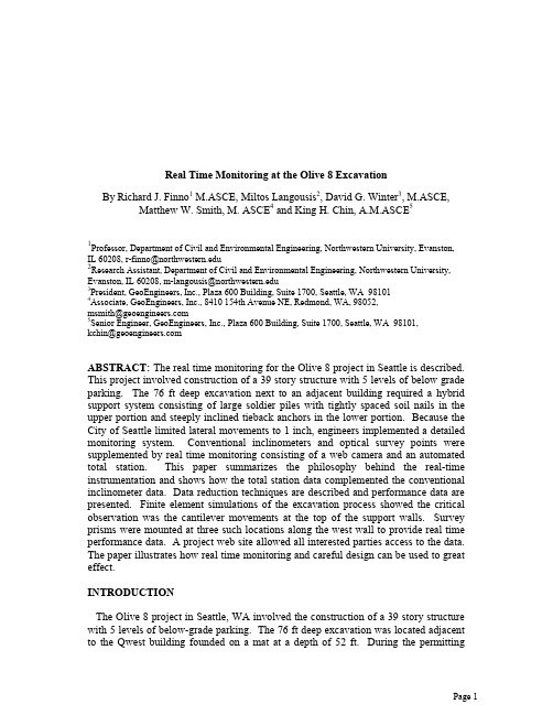
Real Time Monitoring at the Olive 8 Excavation By Richard J. Finno1 M.ASCE, Miltos Langousis2, David G. Winter3, M.ASCE, Matthew W. Smith, M. ASCE4 and King H. Chin, A.M.ASCE5
Py of Seattle stipulated that if the lateral movements were observed to be in excess of ½ inch between two successive readings or if the total wall movements exceeded 1 inch, the construction of the shoring wall would be stopped to evaluate the cause of the movement and to establish the type and extent of remedial measures required. Based on past performance data of excavations through similar soil conditions, typical deflections for excavations of this height (Clough and O’Rourke 1990) were expected to vary from 0.001H to 0.003H, or ¾ inch to about 2.5 inches. Therefore particular attention was paid to designing the support system to limit the movements to less than 1 inch. To meet these requirements, the wall adjacent to the Qwest building was designed with a hybrid support system consisting of large soldier piles with tightly spaced soil nails in the upper portion and steeply inclined tieback anchors in the lower portion. To facilitate timely data acquisition and evaluation during construction, a robotic total station autonomously collected 3-dimensional movements of prisms established at the top of the support wall. These data were placed autonomously on a web site that allowed all interested parties access to the information. The total station data were combined with lateral movements behind the support wall measured with conventional inclinometers. Because design calculations suggested the cantilever movements at the top of the wall could likely have been the largest movements that would occur, the combination of the two types of data would allow essentially real time evaluation of the effects of construction on the ground movements. This paper describes the Olive 8 excavation, discusses the design studies used to develop the instrumentation approach, presents the instrumentation and data acquisition systems employed at the site, summarizes the performance of the support system and compares the design predictions with the observed responses. SITE DESCRIPTION The design of the excavation for the 8th and Olive development in Seattle presented a number of challenges due to the presence of the adjacent Qwest building. A 16 ft alley separated the Olive 8 excavation and the Qwest building, immediately to the west. The Qwest building extends approximately 52 ft below grade and is supported on a perimeter strip footing and a mat foundation for the core of the structure. The design bearing pressure of these foundations was 10 ksf. Existing buried power and communications utilities are located in the alley along with five utility vaults. Because of the movement constraints imposed by these conditions, the design of the excavation support for that wall differed from the other three walls. A cross section through the excavation adjacent to the Qwest building is shown in Figure 1. The shoring system for the west support wall consisted of a combination of soldier piles, soil nails and tiedback ground anchors. The soldier piles were W24x162 sections spaced at approximately 8 ft centers. The upper portion of the alley soils was reinforced with a high density soil nail configuration to the elevation where the tieback anchors were installed. Typically, 9 rows of soil nails were installed at 3 ft vertical by 4 ft horizontal spacing. The soil nails were angled 15 degrees below the horizontal
危大工程监测方案与基坑监控
一、项目背景危大工程监测方案与基坑监控是在工程施工过程中非常重要的一项技术活动,旨在通过对工程施工现场各种监测参数和监测指标的实时、准确、可靠的监测和分析,掌握危大工程施工现场活动规律,及时发现和处理工程施工中存在的风险,确保工程施工安全、顺利、高效进行。
基坑工程是地下工程的一种特殊形式,也是危大工程的一种,其施工难度大、风险高。
基坑施工安全有着特殊的重要意义。
基坑监控作为解决基坑工程施工中的各类地质灾害风险,确保基坑施工安全的一项重要技术手段,被广泛应用于国内外各类基坑工程中。
本文拟针对危大工程监测方案与基坑监控进行研究,探讨其技术要点和技术难点,提出一整套危大工程监测方案与基坑监控技术体系及其相关技术指标,旨在为危大工程监测方案与基坑监控提供一些技术参考和支持,提高危大工程施工安全水平。
二、监测方案的技术要点(一)监测范围和目标危大工程监测方案与基坑监控的监测范围应包括施工现场内、外各种场所和设备,如地下室、基坑、台阶、支撑体系、排水设备、辅助设备等。
监测目标应包括地质变形、土壤稳定性、地下水位、周边建筑结构、施工设备等情况。
(二)监测手段和方法危大工程监测方案与基坑监控的监测手段和方法包括传感器监测、遥感监测、实地测量等技术手段。
其中,传感器监测是指通过各种传感器设备进行实时监测,遥感监测是指通过卫星遥感、无人机遥感等技术手段进行监测,实地测量是指到施工现场进行手工测量等方法。
各种监测手段和方法应根据具体施工环境和监测要求选择和配合使用。
(三)监测指标和标准危大工程监测方案与基坑监控的监测指标和标准应包括地下水位、地下水位变化速度、土壤渗透性、土壤压力、土壤变形、地震烈度等。
各种监测指标和标准应根据当地地质条件和监测要求确定,保障监测准确性和实用性。
(四)监测数据处理和分析危大工程监测方案与基坑监控的监测数据处理和分析应包括数据采集、数据传输、数据处理、数据分析、数据报告等环节。
各种监测数据应通过网络传输、计算机处理等手段进行处理和分析,形成监测数据报告及时反馈给相关部门。
- 1、下载文档前请自行甄别文档内容的完整性,平台不提供额外的编辑、内容补充、找答案等附加服务。
- 2、"仅部分预览"的文档,不可在线预览部分如存在完整性等问题,可反馈申请退款(可完整预览的文档不适用该条件!)。
- 3、如文档侵犯您的权益,请联系客服反馈,我们会尽快为您处理(人工客服工作时间:9:00-18:30)。
国外基坑工程监测方案研究
一、前言
基坑工程是指在地下开挖并临时支护的工程,通常用于地下建筑物或地下结构的施工,如地下停车场、地下商场、地下车站等。
由于基坑工程的复杂性和危险性,必须进行严密的监测工作,以确保施工过程中的安全和稳定性。
本文主要研究国外基坑工程监测方案,探讨国外先进的监测技术和方法,为我国的基坑工程监测提供参考。
二、国外基坑工程监测方案概述
国外基坑工程监测方案通常包括以下几个方面:地质灾害监测、地下水位监测、基坑变形监测、地表沉降监测、环境监测等。
其中,基坑变形监测是最为关键和重要的一个环节,国外常用的监测方法包括GPS监测、测斜仪监测、地下水压力监测、顶管测量等。
下面将对这些监测方法进行详细介绍。
三、 GPS监测
GPS监测是一种利用全球定位系统(GPS)技术对基坑工程变形进行实时监测的方法。
GPS监测系统通常由多个GPS接收器组成,这些接收器分布在基坑工程的周边或者在基坑内部的关键位置。
通过对这些GPS接收器的连续监测和数据分析,可以实时、准确地获得基坑工程的变形情况,为施工管理和安全预警提供重要依据。
国外一些先进的GPS监测系统还具有自动报警和远程监控功能,一旦监测数据出现异常,可以立即通过手机或电脑接收到报警信息,从而及时采取措施,避免事故发生。
GPS监测系统的优点在于监测精度高、实时性强、操作简便,因此在国外的基坑工程监测中得到了广泛应用。
四、测斜仪监测
测斜仪监测是一种利用倾斜传感器对基坑工程支护结构的倾斜变化进行监测的方法。
国外常用的测斜仪包括电子倾角仪、水准仪等,这些仪器可以精确地测量支护结构在垂直方向上的倾斜情况,为基坑工程的变形监测提供重要数据。
测斜仪监测系统的特点在于安装方便、监测可靠、成本低廉,因此在国外的基坑工程监测中得到了广泛应用。
国外一些先进的测斜仪监测系统还可以实现远程数据传输和自动报警功能,因此在基坑工程的实时监测中发挥了重要作用。
五、地下水压力监测
地下水压力监测是一种利用水压力传感器对基坑工程周边的地下水位和水压力进行监测的方法。
地下水位和水压力的变化是导致基坑工程变形和失稳的重要因素,因此对地下水位和水压力进行实时监测是非常重要的。
国外一些先进的地下水压力监测系统可以利用无线传感器网络实现基坑周边地下水压力的
实时监测和远程数据传输。
这些监测系统还可以通过预置的阈值进行自动报警和远程控制,从而及时发现地下水位异常,保障基坑工程的安全。
六、顶管测量
顶管测量是一种利用激光测距仪对基坑工程顶部支撑结构的变形进行监测的方法。
通过对
顶部支撑结构进行连续测量和数据分析,可以获得基坑工程在水平和垂直方向上的变形情况,为基坑工程的变形监测提供重要数据。
国外一些先进的顶管测量系统采用了先进的激光测距仪和高精度的数据处理算法,可以实
现基坑工程变形的实时监测和数据分析。
这些系统通常具有自动报警和远程监控功能,在
基坑工程的安全管理中发挥了重要作用。
七、结论
基坑工程的监测是保障施工安全和工程质量的重要环节,国外已经发展出了一系列先进的
监测技术和方法。
本文通过对国外基坑工程监测方案的研究,对我国的基坑工程监测提出
了一些借鉴和启示。
希望我国的基坑工程监测能够通过引进国外先进技术和方法,进一步
提高监测水平,保障施工安全和工程质量。