abaqus子结构帮助文档

合集下载

ABAQUS

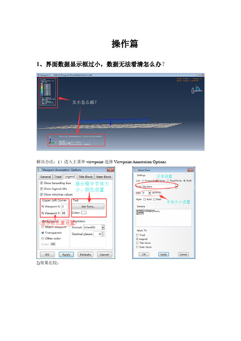
操作篇1、界面数据显示框过小，数据无法看清怎么办？解决办法：1）进入主菜单viewpoint选择Viewpoint Annotation Options 2)效果比较：说明：主菜单中Viewpoint选项中还可以修改显示界面的形式，在模型上添加注释（Annotation），修改数据显示框的位置、大小、形式等等。

2、如何查看节点或单元在模型中的位置？解决办法：1）在主菜单View栏下选中Toolbars，进而选中coustomize编辑框，选中“Group Display”则在主界面生成Group Display快捷操作框。

2）点击”create group display”进入对话框，可以查找相应编号的节点或单元在模型中的具体位置3、分析结果中，显示的位移过大或者过小应该如何调整？解决方法：在界面左边快捷栏点击“common options”4、梁截面定义** Section: Section-1-ADSET3 Profile: Profile-1*Beam Section, elset=ADSET3, material=MATERIAL-2,temperature=GRADIENTS, section=L0.12275, 0.12275, 0.007944, 0.007944 （a,b,t1,t2）-0.883444,-0.468537,0.5、定义表面时“SNEG”“SPOS”表达的含义？*Surface, type=ELEMENT, name=SURF-1_SURF-1_SNEG, SNEG*Surface, type=ELEMENT, name=SURF-1_SURF-1_SPOS_1, SPOS（SNEG/ SPOS的作用是什么？）解答：Refers to the sides of the elements in the surface.用来指定选择的接触面。

EG:6、RigidBody约束和刚体部件的差别在于：刚体部件同部件相关联，RigidBody约束同组装实体中的区域相关联。

ABAQUS使用手册（中文版）

ABAQUS使用手册（中文版）ABAQUS入门使用手册ABAQUS简介：ABAQUS是一套先进的通用有限元程序系统，这套软件的目的是对固体和结构的力学问题进行数值计算分析，而我们将其用于材料的计算机模拟及其前后处理，主要得益于ABAQUS给我们的ABAQUS/Standard及ABAQUS/Explicit通用分析模块。

ABAQUS有众多的分析模块，我们使用的模块主要是ABAQUS/CAE及Viewer,前者用于建模及相应的前处理，后者用于对结果进行分析及处理。

下面将对这两个模块的使用结合本人的体会做一些具体的说明：一．ABAQUS/CAECAE模块用于分析对象的建模，特性及约束条件的给定，网格的划分以及数据传输等等，其核心由七个步骤组成，下面将对这七个步骤作出说明：1.PART步（1）Part→CreatModeling Space:①3D代表三维②2D代表二维③Aaxisymmetric代表轴对称，这三个选项的选定要视所模拟对象的结构而定。

Type: ①Deformable为一般选项，适合于绝大多数的模拟对象。

②Discrete rigid 和Analytical rigid用于多个物体组合时，与我们所研究的对象相关的物体上。

ABAQUS假设这些与所研究的对象相关的物体均为刚体，对于其中较简单的刚体，如球体而言，选择前者即可。

若刚体形状较复杂，或者不是规则的几何图形，那么就选择后者。

需要说明的是，由于后者所建立的模型是离散的，所以只能是近似的，不可能和实际物体一样，因此误差较大。

Shape中有四个选项，其排列规则是按照维数而定的，可以根据我们的模拟对象确定。

Type: ①Extrusion用于建立一般情况的三维模型②Revolution建立旋转体模型③Sweep用于建立形状任意的模型。

Approximate size:在此栏中设定作图区的大致尺寸，其单位与我们选定的单位一致。

设置完毕，点击Continue进入作图区。

abaqus帮助文档翻译 2.1.11 一摞积木在通用接触下的倒塌分析

2.1.11 Collapse of a stack of blocks with general contactProduct: Abaqus/ExplicitThis example illustrates the use of the general contact capability in a simulation involving a large number of contacting bodies. The general contact algorithm allows very simple definitions of contact with very few restrictions on the types of surfaces involved (see “Defining general contact interactions in Abaqus/Explicit,” Section 35.4.1 of the Abaqus Analysis User's Manual).Problem descriptionThe model simulates the collapse of a stack of blocks. The undeformed configuration of the model is shown in Figure 2.1.11–1. There are 35 blocks, and each block is 12.7 × 12.7 × 76.2 mm (0.5 × 0.5 × 3 inches) in size. The blocks are stacked on a rigid floor. The stack is subjected to gravity loading. It is assumed that a key block near the bottom of the stack has been removed just before the start of the analysis, initiating the collapse.Each block is modeled with a single C3D8R element. The use of a coarse mesh highlights the edge-to-edge contact capability of the general contact algorithm, because the majority of the block-to-block interactions do not result in penetrations of nodes into faces.Two different cases are analyzed. In the first analysis the blocks are rigid. In the second analysis the blocks are deformable. In the latter case, the material of the block is assumed to be linear elastic with a Young's modulus of 12.135 GPa (1.76 × 106 Psi), a Poisson's ratio of 0.3, and a density of 577.098 kg/m3 (5.4 × 10–5 lb s2/in4). Only the density is relevant for the analysis assuming rigid blocks. In addition, ENHANCED hourglass control is used for the deformable analysis. The rigid floor is modeled as a discrete rigid surface using a single R3D4 element.This model involves a large number of contacting bodies. The general contact capability greatly simplifies the contact definition, since each of the 595 possible block-to-block pairings does not need to be specified individually. The general contact inclusions option to automatically define an all-inclusive surface is used and is the simplest way to define contact in the model. Coulomb friction with a friction coefficient of 0.15 is assumed between the individual blocks and between the blocks and floor. The general contact property assignment is used to assign this nondefault contact property.By default, the general contact algorithm in Abaqus/Explicit accounts foredge-to-edge contact of perimeter edges on structural elements. Geometric featureedges of a model can also be considered for edge-to-edge contact by the general contact algorithm; including the geometric feature edges is crucial in this analysis. A cutoff feature angle of 20° is specified for the feature angle criterion of the surface property to indicate that all edges with feature angles greater than 20° should be considered for edge-to-edge contact. The feature angle is the angle formed between the normals of the two facets connected to an edge.The magnitude of the gravity loading is increased by a factor of 10 to facilitate demonstration of the edge-to-edge contact capability with a short analysis time. The analysis is performed for a period of 0.15 seconds. For the analysis with rigid blocks there is no deformable element available in the model to control the stable time increment. A fixed time increment of 1 × 10–6 seconds is specified for this purpose, which is similar to the time increment used by the analysis with deformable blocks. The time increment chosen for the analysis with rigid blocks will affect the penalty stiffness used by the contact algorithm since the penalty stiffness is inversely proportional to the time increment squared.Results and discussionResults are shown for the rigid body case. Results for the deformable case are very similar to the rigid model results.Figure 2.1.11–2 shows the displaced shape of the block assembly after 0.0375 seconds. The stack of blocks has started to collapse under gravity loading. Figure2.1.11–3 shows a close-up view of the collapsing blocks after 0.1125 seconds. This figure clearly shows that the geometric feature edges of individual blocks contact each other during collapse. Figure 2.1.11–4 shows the final configuration of the blocks. The stack has collapsed completely on the rigid surface.Input filesblocks_rigid_gcont.inpInput file for the rigid body analysis.blocks_rigid_assembly.inpExternal file referenced by the rigid body analysis.blocks_deform_gcont.inpInput file for the deformable analysis.blocks_deform_assembly.inpExternal file referenced by the deformable analysis.FiguresFigure 2.1.11–1 Initial configuration of the stack of blocks.Figure 2.1.11–2 Displaced shape after 0.0375 s.Figure 2.1.11–3 Close-up view of the collapsing blocks after 0.1125 s.Figure 2.1.11–4 Final configuration of the model.2.1.11 一摞积木在通用接触下的倒塌分析Product：Abaqus/Explicit这个例子说明通用接触的使用在涉及大量接触物体倒塌的模拟中应用。

Abaqus User Subroutines Reference Guide 用户材料子程序帮助文档

1.1.41 UMATUser subroutine to define a material's mechanical behavior.Product: Abaqus/StandardWarning: The use of this subroutine generally requires considerable expertise. Y ou arecautioned that the implementation of any realistic constitutive model requires extensivedevelopment and testing. Initial testing on a single-element model with prescribedtraction loading is strongly recommended.References“User-defined mechanical material behavior,” Section 26.7.1 of the Abaqus Analysis User's Guide“User-defined thermal material behavior,” Section 26.7.2 of the Abaqus Analysis User's Guide*USER MA TERIAL“S D V I N I,” Section 4.1.11 of the Abaqus V erification Guide“U M A T and U H Y P E R,” Section 4.1.21 of the Abaqus V erification GuideOv erv iewUser subroutine U M A T:can be used to define the mechanical constitutive behavior of a material;will be called at all material calculation points of elements for which the material definition includes auser-defined material behavior;can be used with any procedure that includes mechanical behavior;can use solution-dependent state variables;must update the stresses and solution-dependent state variables to their values at the end of theincrement for which it is called;must provide the material Jacobian matrix, , for the mechanical constitutive model;can be used in conjunction with user subroutine U S D F L D to redefine any field variables before they are passed in; andis described further in “User-defined mechanical material behavior,” Section 26.7.1 of the AbaqusAnalysis User's Guide.Storage of stress and strain componentsIn the stress and strain arrays and in the matrices D D S D D E, D D S D D T, and D R P L D E, direct components are stored first, followed by shear components. There are N D I direct and N S H R engineering shear components. The order of the components is defined in “Conventions,” Section 1.2.2 of the Abaqus Analysis User's Guide. Since the number of active stress and strain components varies between element types, the routine must be coded toprovide for all element types with which it will be used.Defining local orientationsIf a local orientation (“Orientations,” Section 2.2.5 of the Abaqus Analysis User's Guide) is used at the same point as user subroutine U M A T, the stress and strain components will be in the local orientation; and, in the case of finite-strain analysis, the basis system in which stress and strain components are stored rotates with the material.StabilityY ou should ensure that the integration scheme coded in this routine is stable—no direct provision is made to include a stability limit in the time stepping scheme based on the calculations in U M A T.Convergence rateD D S D DE and—for coupled temperature-displacement and coupled thermal-electrical-structural analyses—D D S D D T, D R P L D E, and D R P L D T must be defined accurately if rapid convergence of the overall Newton scheme is to be achieved. In most cases the accuracy of this definition is the most important factor governing the convergence rate. Since nonsymmetric equation solution is as much as four times as expensive as the corresponding symmetric system, if the constitutive Jacobian (D D S D D E) is only slightly nonsymmetric (for example, a frictional material with a small friction angle), it may be less expensive computationally to use a symmetric approximation and accept a slower convergence rate.An incorrect definition of the material Jacobian affects only the convergence rate; the results (if obtained) are unaffected.Special considerations for various element typesThere are several special considerations that need to be noted.A v ailability of deformation gradientThe deformation gradient is available for solid (continuum) elements, membranes, and finite-strain shells(S3/S3R, S4, S4R, SAXs, and SAXAs). It is not available for beams or small-strain shells. It is stored as a 3× 3 matrix with component equivalence D F G R D0(I,J). For fully integrated first-order isoparametric elements (4-node quadrilaterals in two dimensions and 8-node hexahedra in three dimensions) the selectively reduced integration technique is used (also known as the technique). Thus, a modified deformation gradientis passed into user subroutine U M A T. For more details, see “Solid isoparametric quadrilaterals and hexahedra,”Section 3.2.4 of the Abaqus Theory Guide.Beams and shells that calculate transv erse shear energyIf user subroutine U M A T is used to describe the material of beams or shells that calculate transverse shear energy, you must specify the transverse shear stiffness as part of the beam or shell section definition to define the transverse shear behavior. See “Shell section behavior,” Section 29.6.4 of the Abaqus Analysis User's Guide, and “Choosing a beam element,” Section 29.3.3 of the Abaqus Analysis User's Guide, for informationon specifying this stiffness.Open-section beam elementsWhen user subroutine U M A T is used to describe the material response of beams with open sections (for example, an I-section), the torsional stiffness is obtained aswhere J is the torsional constant, A is the section area, k is a shear factor, and is the user-specified transverse shear stiffness (see “Transverse shear stiffness definition” in “Choosing a beam element,” Section29.3.3 of the Abaqus Analysis User's Guide).E lements w ith hourglassing modesIf this capability is used to describe the material of elements with hourglassing modes, you must define the hourglass stiffness factor for hourglass control based on the total stiffness approach as part of the element section definition. The hourglass stiffness factor is not required for enhanced hourglass control, but you can define a scaling factor for the stiffness associated with the drill degree of freedom (rotation about the surface normal). See “Section controls,” Section 27.1.4 of the Abaqus Analysis User's Guide, for information on specifying the stiffness factor.Pipe-soil interaction elementsThe constitutive behavior of the pipe-soil interaction elements (see “Pipe-soil interaction elements,” Section 32.12.1 of the Abaqus Analysis User's Guide) is defined by the force per unit length caused by relative displacement between two edges of the element. The relative-displacements are available as “strains” (S T R A N and D S T R A N). The corresponding forces per unit length must be defined in the S T R E S S array. The Jacobian matrix defines the variation of force per unit length with respect to relative displacement.For two-dimensional elements two in-plane components of “stress” and “strain” exist (N T E N S=N D I=2, andN S H R=0). For three-dimensional elements three components of “stress” and “strain” exist (N T E N S=N D I=3, and N S H R=0).Large volume changes with geometric nonlinearityIf the material model allows large volume changes and geometric nonlinearity is considered, the exact definition of the consistent Jacobian should be used to ensure rapid convergence. These conditions are most commonly encountered when considering either large elastic strains or pressure-dependent plasticity. In the former case, total-form constitutive equations relating the Cauchy stress to the deformation gradient are commonly used; in the latter case, rate-form constitutive laws are generally used.For total-form constitutive laws, the exact consistent Jacobian is defined through the variation in Kirchhoff stress:Here, J is the determinant of the deformation gradient, is the Cauchy stress, is the virtual rate of deformation, and is the virtual spin tensor, defined asFor rate-form constitutive laws, the exact consistent Jacobian is given byUse with incompressible elastic materialsFor user-defined incompressible elastic materials, user subroutine U H Y P E R should be used rather than user subroutine U M A T. In U M A T incompressible materials must be modeled via a penalty method; that is, you must ensure that a finite bulk modulus is used. The bulk modulus should be large enough to model incompressibility sufficiently but small enough to avoid loss of precision. As a general guideline, the bulk modulus should be about – times the shear modulus. The tangent bulk modulus can be calculated fromIf a hybrid element is used with user subroutine U M A T, Abaqus/Standard will replace the pressure stress calculated from your definition of S T R E S S with that derived from the Lagrange multiplier and will modify the Jacobian appropriately.For incompressible pressure-sensitive materials the element choice is particularly important when using user subroutine U M A T. In particular, first-order wedge elements should be avoided. For these elements the technique is not used to alter the deformation gradient that is passed into user subroutine U M A T, which increases the risk of volumetric locking.Increments for which only the Jacobian can be definedAbaqus/Standard passes zero strain increments into user subroutine U M A T to start the first increment of all the steps and all increments of steps for which you have suppressed extrapolation (see “Defining an analysis,”Section 6.1.2 of the Abaqus Analysis User's Guide). In this case you can define only the Jacobian (D D S D D E).Utility routinesSeveral utility routines may help in coding user subroutine U M A T. Their functions include determining stress invariants for a stress tensor and calculating principal values and directions for stress or strain tensors. These utility routines are discussed in detail in “Obtaining stress invariants, principal stress/strain values and directions, and rotating tensors in an Abaqus/Standard analysis,” Section 2.1.11.U ser subroutine interfaceS U B R O U T I N E U M A T(S T R E S S,S T A T E V,D D S D D E,S S E,S P D,S C D,1R P L,D D S D D T,D R P L D E,D R P L D T,2S T R A N,D S T R A N,T I M E,D T I M E,T E M P,D T E M P,P R E D E F,D P R E D,C M N A M E,3N D I,N S H R,N T E N S,N S T A T V,P R O P S,N P R O P S,C O O R D S,D R O T,P N E W D T,4C E L E N T,D F G R D0,D F G R D1,N O E L,N P T,L A Y E R,K S P T,K S T E P,K I N C)CI N C L U D E'A B A_P A R A M.I N C'C H A R A C T E R*80C M N A M ED I ME N S I O N S T R E S S(N T E N S),S T A T E V(N S T A T V),1D D S D D E(N T E N S,N T E N S),D D S D D T(N T E N S),D R P L D E(N T E N S),2S T R A N(N T E N S),D S T R A N(N T E N S),T I M E(2),P R E D E F(1),D P R E D(1),3P R O P S(N P R O P S),C O O R D S(3),D R O T(3,3),D F G R D0(3,3),D F G R D1(3,3)user coding to define D D S D D E,S T R E S S,S T A T E V,S S E,S P D,S C Dand, if necessary,R P L,D D S D D T,D R P L D E,D R P L D T,P N E W D TR E T U R NE N DV ariables to be definedIn all situationsD D S D D E(N TE N S,N T E N S)Jacobian matrix of the constitutive model, , where are the stress increments and are the strain increments. D D S D D E(I,J) defines the change in the I th stress component at the end of the time increment caused by an infinitesimal perturbation of the J th component of the strain increment array.Unless you invoke the unsymmetric equation solution capability for the user-defined material,Abaqus/Standard will use only the symmetric part of D D S D D E. The symmetric part of the matrix iscalculated by taking one half the sum of the matrix and its transpose.S T R E S S(N T E N S)This array is passed in as the stress tensor at the beginning of the increment and must be updated in this routine to be the stress tensor at the end of the increment. If you specified initial stresses (“Initial conditions in Abaqus/Standard and Abaqus/Explicit,” Section 34.2.1 of the Abaqus Analysis User's Guide), this array will contain the initial stresses at the start of the analysis. The size of this array depends on the value of N T E N S as defined below. In finite-strain problems the stress tensor has already been rotated to account for rigid body motion in the increment before U M A T is called, so that only the corotational part of the stress integration should be done in U M A T. The measure of stress used is “true” (Cauchy) stress.S T A T E V(N S T A T V)An array containing the solution-dependent state variables. These are passed in as the values at thebeginning of the increment unless they are updated in user subroutines U S D F L D or U E X P A N, in which case the updated values are passed in. In all cases S T A T E V must be returned as the values at the end of the increment. The size of the array is defined as described in “Allocating space” in “User subroutines:overview,” Section 18.1.1 of the Abaqus Analysis User's Guide.In finite-strain problems any vector-valued or tensor-valued state variables must be rotated to account for rigid body motion of the material, in addition to any update in the values associated with constitutivebehavior. The rotation increment matrix, D R O T, is provided for this purpose.S S E,S P D,S C DSpecific elastic strain energy, plastic dissipation, and “creep” dissipation, respectively. These are passed in as the values at the start of the increment and should be updated to the corresponding specific energy values at the end of the increment. They have no effect on the solution, except that they are used forenergy output.Only in a fully coupled thermal-stress or a coupled thermal-electrical-structural analysisR P LV olumetric heat generation per unit time at the end of the increment caused by mechanical working of the material.D D S D D T(N TE N S)V ariation of the stress increments with respect to the temperature.D R P L D E(N TE N S)V ariation of R P L with respect to the strain increments.D R P L D TV ariation of R P L with respect to the temperature.Only in a geostatic stress procedure or a coupled pore fluid diffusion/stress analysis for pore pressure cohesive elementsR P LR P L is used to indicate whether or not a cohesive element is open to the tangential flow of pore fluid. Set R P L equal to 0 if there is no tangential flow; otherwise, assign a nonzero value to R P L if an element is open.Once opened, a cohesive element will remain open to the fluid flow.V ariable that can be updatedP N E W D TRatio of suggested new time increment to the time increment being used (D T I M E, see discussion later in this section). This variable allows you to provide input to the automatic time incrementation algorithms in Abaqus/Standard (if automatic time incrementation is chosen). For a quasi-static procedure the automatic time stepping that Abaqus/Standard uses, which is based on techniques for integrating standard creep laws (see “Quasi-static analysis,” Section 6.2.5 of the Abaqus Analysis User's Guide), cannot becontrolled from within the U M A T subroutine.P N E W D T is set to a large value before each call to U M A T.If P N E W D T is redefined to be less than 1.0, Abaqus/Standard must abandon the time increment andattempt it again with a smaller time increment. The suggested new time increment provided to theautomatic time integration algorithms is P N E W D T × D T I M E, where the P N E W D T used is the minimum value for all calls to user subroutines that allow redefinition of P N E W D T for this iteration.If P N E W D T is given a value that is greater than 1.0 for all calls to user subroutines for this iteration and the increment converges in this iteration, Abaqus/Standard may increase the time increment. The suggestednew time increment provided to the automatic time integration algorithms is P N E W D T × D T I M E, where the P N E W D T used is the minimum value for all calls to user subroutines for this iteration.If automatic time incrementation is not selected in the analysis procedure, values of P N E W D T that aregreater than 1.0 will be ignored and values of P N E W D T that are less than 1.0 will cause the job to terminate. V ariables passed in for informationS T R A N(N T E N S)An array containing the total strains at the beginning of the increment. If thermal expansion is included in the same material definition, the strains passed into U M A T are the mechanical strains only (that is, thethermal strains computed based upon the thermal expansion coefficient have been subtracted from the total strains). These strains are available for output as the “elastic” strains.In finite-strain problems the strain components have been rotated to account for rigid body motion in the increment before U M A T is called and are approximations to logarithmic strain.D S T R A N(N TE N S)Array of strain increments. If thermal expansion is included in the same material definition, these are the mechanical strain increments (the total strain increments minus the thermal strain increments).T I M E(1)V alue of step time at the beginning of the current increment or frequency.T I M E(2)V alue of total time at the beginning of the current increment.D T I M ETime increment.T E M PTemperature at the start of the increment.D TE M PIncrement of temperature.P R E D E FArray of interpolated values of predefined field variables at this point at the start of the increment, based on the values read in at the nodes.D P RE DArray of increments of predefined field variables.C M N A M EUser-defined material name, left justified. Some internal material models are given names starting with the “ABQ_” character string. To avoid conflict, you should not use “ABQ_” as the leading string for C M N A M E. N D INumber of direct stress components at this point.N S H RNumber of engineering shear stress components at this point.N T E N SSize of the stress or strain component array (N D I + N S H R).N S T A T VNumber of solution-dependent state variables that are associated with this material type (defined asdescribed in “Allocating space” in “User subroutines: overview,” Section 18.1.1 of the Abaqus Analysis User's Guide).P R O P S(N P R O P S)User-specified array of material constants associated with this user material.N P R O P SUser-defined number of material constants associated with this user material.C O O RD SAn array containing the coordinates of this point. These are the current coordinates if geometricnonlinearity is accounted for during the step (see “Defining an analysis,” Section 6.1.2 of the Abaqus Analysis User's Guide); otherwise, the array contains the original coordinates of the point.D R O T(3,3)Rotation increment matrix. This matrix represents the increment of rigid body rotation of the basis system in which the components of stress (S T R E S S) and strain (S T R A N) are stored. It is provided so that vector-or tensor-valued state variables can be rotated appropriately in this subroutine: stress and straincomponents are already rotated by this amount before U M A T is called. This matrix is passed in as a unit matrix for small-displacement analysis and for large-displacement analysis if the basis system for thematerial point rotates with the material (as in a shell element or when a local orientation is used).C E L E N TCharacteristic element length, which is a typical length of a line across an element for a first-order element;it is half of the same typical length for a second-order element. For beams and trusses it is a characteristic length along the element axis. For membranes and shells it is a characteristic length in the referencesurface. For axisymmetric elements it is a characteristic length in the plane only. For cohesiveelements it is equal to the constitutive thickness.D F G R D0(3,3)Array containing the deformation gradient at the beginning of the increment. If a local orientation is defined at the material point, the deformation gradient components are expressed in the local coordinate system defined by the orientation at the beginning of the increment. For a discussion regarding the availability of the deformation gradient for various element types, see “Availability of deformation gradient.”D F G R D1(3,3)Array containing the deformation gradient at the end of the increment. If a local orientation is defined at the material point, the deformation gradient components are expressed in the local coordinate system defined by the orientation. This array is set to the identity matrix if nonlinear geometric effects are not included in the step definition associated with this increment. For a discussion regarding the availability of thedeformation gradient for various element types, see “Availability of deformation gradient.”N O E LElement number.N P TIntegration point number.L A Y E RLayer number (for composite shells and layered solids).K S P TSection point number within the current layer.K S T E PStep number.K I N CIncrement number.Example: Using more than one user-defined mechanical material modelTo use more than one user-defined mechanical material model, the variable C M N A M E can be tested for different material names inside user subroutine U M A T as illustrated below:I F(C M N A M E(1:4).E Q.'M A T1')T H E NC A L L U M A T_M A T1(argument_list)E L S E I F(C M N A M E(1:4).E Q.'M A T2')T H E NC A L L U M A T_M A T2(argument_list)E N D I FU M A T_M A T1 and U M A T_M A T2 are the actual user material subroutines containing the constitutive material models for each material M A T1 and M A T2, respectively. Subroutine U M A T merely acts as a directory here. The argument list may be the same as that used in subroutine U M A T.Example: Simple linear viscoelastic materialAs a simple example of the coding of user subroutine U M A T, consider the linear, viscoelastic model shown in Figure 1.1.41–1. Although this is not a very useful model for real materials, it serves to illustrate how to code the routine.Figure 1.1.41–1 Simple linear viscoelastic model.The behavior of the one-dimensional model shown in the figure iswhere and are the time rates of change of stress and strain. This can be generalized for small straining of an isotropic solid asandwhereand , , , , and are material constants ( and are the Lamé constants).A simple, stable integration operator for this equation is the central difference operator:where f is some function, is its value at the beginning of the increment, is the change in the function over the increment, and is the time increment.Applying this to the rate constitutive equations above givesandso that the Jacobian matrix has the termsandThe total change in specific energy in an increment for this material iswhile the change in specific elastic strain energy iswhere D is the elasticity matrix:No state variables are needed for this material, so the allocation of space for them is not necessary. In a morerealistic case a set of parallel models of this type might be used, and the stress components in each model might be stored as state variables.For our simple case a user material definition can be used to read in the five constants in the order , , , , and so thatThe routine can then be coded as follows:S U B R O U T I N E U M A T(S T R E S S,S T A T E V,D D S D D E,S S E,S P D,S C D,1R P L,D D S D D T,D R P L D E,D R P L D T,2S T R A N,D S T R A N,T I M E,D T I M E,T E M P,D T E M P,P R E D E F,D P R E D,C M N A M E,3N D I,N S H R,N T E N S,N S T A T V,P R O P S,N P R O P S,C O O R D S,D R O T,P N E W D T,4C E L E N T,D F G R D0,D F G R D1,N O E L,N P T,L A Y E R,K S P T,K S T E P,K I N C)CI N C L U D E'A B A_P A R A M.I N C'CC H A R A C T E R*80C M N A M ED I ME N S I O N S T R E S S(N T E N S),S T A T E V(N S T A T V),1D D S D D E(N T E N S,N T E N S),2D D S D D T(N T E N S),D R P L D E(N T E N S),3S T R A N(N T E N S),D S T R A N(N T E N S),T I M E(2),P R E D E F(1),D P R E D(1),4P R O P S(N P R O P S),C O O R D S(3),D R O T(3,3),D F G R D0(3,3),D F G R D1(3,3)D I ME N S I O N D S T R E S(6),D(3,3)CC E V A L U A T E N E W S T R E S S T E N S O RCE V=0.D E V=0.D O K1=1,N D IE V=E V+S T R A N(K1)D E V=D E V+D S T R A N(K1)E N D D OCT E R M1=.5*D T I M E+P R O P S(5)T E R M1I=1./T E R M1T E R M2=(.5*D T I M E*P R O P S(1)+P R O P S(3))*T E R M1I*D E VT E R M3=(D T I M E*P R O P S(2)+2.*P R O P S(4))*T E R M1ICD O K1=1,N D ID S T RE S(K1)=T E R M2+T E R M3*D S T R A N(K1)1+D T I M E*T E R M1I*(P R O P S(1)*E V2+2.*P R O P S(2)*S T R A N(K1)-S T R E S S(K1))S T R E S S(K1)=S T R E S S(K1)+D S T R E S(K1)E N D D OCT E R M2=(.5*D T I M E*P R O P S(2)+P R O P S(4))*T E R M1II1=N D ID O K1=1,N S H RI1=I1+1D S T RE S(I1)=T E R M2*D S T R A N(I1)+1D T I M E*T E R M1I*(P R O P S(2)*S T R A N(I1)-S T R E S S(I1)) S T R E S S(I1)=S T R E S S(I1)+D S T R E S(I1)E N D D OCC C R E A T E N E W J A C O B I A NCT E R M2=(D T I M E*(.5*P R O P S(1)+P R O P S(2))+P R O P S(3)+12.*P R O P S(4))*T E R M1IT E R M3=(.5*D T I M E*P R O P S(1)+P R O P S(3))*T E R M1ID O K1=1,N TE N SD O K2=1,N TE N SD D S D D E(K2,K1)=0.E N D D OE N D D OCD O K1=1,N D ID D S D D E(K1,K1)=TE R M2E N D D OCD O K1=2,N D IN2=K1–1D O K2=1,N2D D S D D E(K2,K1)=TE R M3D D S D D E(K1,K2)=TE R M3E N D D OE N D D OT E R M2=(.5*D T I M E*P R O P S(2)+P R O P S(4))*T E R M1II1=N D ID O K1=1,N S H RI1=I1+1D D S D D E(I1,I1)=TE R M2E N D D OCC T O T A L C H A N G E I N S P E C I F I C E N E R G YCT D E=0.D O K1=1,N TE N ST D E=T D E+(S T R E S S(K1)-.5*D S T R E S(K1))*D S T R A N(K1)E N D D OCC C H A N G E I N S P E C I F I C E L A S T I C S T R A I N E N E R G YCT E R M1=P R O P S(1)+2.*P R O P S(2)D O K1=1,N D ID(K1,K1)=T E R M1E N D D OD O K1=2,N D IN2=K1-1D O K2=1,N2D(K1,K2)=P R O P S(1)D(K2,K1)=P R O P S(1)E N D D OE N D D OD E E=0.D O K1=1,N D IT E R M1=0.T E R M2=0.D O K2=1,N D IT E R M1=T E R M1+D(K1,K2)*S T R A N(K2)T E R M2=T E R M2+D(K1,K2)*D S T R A N(K2)E N D D OD E E=D E E+(T E R M1+.5*T E R M2)*D S T R A N(K1)E N D D OI1=N D ID O K1=1,N S H RI1=I1+1D E E=D E E+P R O P S(2)*(S T R A N(I1)+.5*D S T R A N(I1))*D S T R A N(I1)E N D D OS S E=S S E+D E ES C D=S C D+T D E– D E ER E T U R NE N D。

abaqus帮助文档_friction

Specifying frictional behavior for mechanical contact property options You can specify a friction model that defines the force resisting the relative tangential motion of the surfaces in a mechanical contact analysis. For more information, see �Frictional behavior,�Section 35.1.5 of the Abaqus Analysis User's Manual.To specify frictional behavior:1. From the main menu bar, select Interaction Property Create.2. In the Create Interaction Property dialog box that appears, do thefollowing:∙Name the interaction property. For more information aboutnaming objects, see �Using basic dialog boxcomponents,�Section 3.2.1.∙Select the Contact type of interaction property.3. Click Continue to close the Create Interaction Property dialog box.4. From the menu bar in the contact property editor, select MechanicalTangential Behavior.5. In the editor that appears, click the arrow to the right of the Frictionformulation field, and select how you want to define friction betweenthe contact surfaces:∙Select Frictionless if you want Abaqus to assume that surfaces in contact slide freely without friction.∙Select Penalty to use a stiffness (penalty) method that permits some relative motion of the surfaces (an “elastic slip”) when theyshould be sticking. While the surfaces are sticking (i.e., ),the magnitude of sliding is limited to this elastic slip. Abaqus willcontinually adjust the magnitude of the penalty constraint toenforce this condition. For more information, see �Stiffnessmethod for imposing frictional constraints in Abaqus/Standard” in“Frictional behavior,�Section 35.1.5 of the Abaqus AnalysisUser's Manual, and �Stiffness method for imposing frictionalconstraints in Abaqus/Explicit” in “Frictional behavior,�Section35.1.5 of the Abaqus Analysis User's Manual.∙Select Static-Kinetic Exponential Decay to specify static and kinetic friction coefficients directly. In this model it is assumedthat the friction coefficient decays exponentially from the staticvalue to the kinetic value. Alternatively, you can enter test data tofit the exponential model. (This Friction formulation option alsoallows you to specify elastic slip.) For more information,see �Specifying static and kinetic friction coefficients” in“Frictional behavior,�Section 35.1.5 of the Abaqus AnalysisUser's Manual.∙Select Rough to specify an infinite coefficient of friction. For more information, see �Preventing slipping regardless ofconta ct pressure” in “Frictional behavior,�Section 35.1.5 of theAbaqus Analysis User's Manual.∙Select Lagrange Multiplier (Standard only) to enforce the sticking constraints at an interface between two surfaces usingthe Lagrange multiplier implementation. With this method there isno relative motion between two closed surfaces until .For more information, see �Lagrange multiplier method forimposing frictional constraints in Abaqus/Standard” in “Frictionalbehavior,�Section 35.1.5 of the Abaqus Analysis User'sManual.∙Select User-defined to define the shear interaction between the contact surfaces with user subroutine FRIC or VFRIC. For moreinformation, see �User-defined friction model” in “Frictionalbehavior,�Section 35.1.5 of the Abaqus Analysis User'sManual.6. If you selected the Penalty or Lagrange Multiplier (Standardonly) friction formulation, perform the following steps:a. Display the Friction tabbed page.b. Choose the Directionality:∙Choose Isotropic to enter a uniform friction coefficient.∙Choose Anisotropic (Standard only) to allow fordifferent friction coefficients in the two orthogonaldirections on the contact surface. For more information,see �Using the anisotropic friction model inAbaqus/Standard” in “Frictional behavior,�Section35.1.5 of the Abaqus Analysis User's Manual.c. Toggle on Use slip-rate-dependent data if the frictioncoefficient is dependent on slip rate.d. Toggle on Use contact-pressure-dependent data if the frictioncoefficient is dependent on the contact pressure.e. Toggle on Use temperature-dependent data if the frictioncoefficient is dependent on temperature.f. Click the arrows to the right of the Number of fieldvariables field to specify the number of field variables on whichthe friction coefficient depends.g. Enter the required data in the data table provided.h. Display the Shear Stress tabbed page, and choose a Shearstress limit option:∙Choose No limit if you do not want to limit the shearstress that can be carried by the interface before thesurfaces begin to slide.∙Choose Specify to enter an equivalent shear stresslimit, . If you choose this option, sliding will occur ifthe magnitude of the equivalent shear stress reaches thisvalue, regardless of the magnitude of the contact pressurestress. For more information, see �Using the optionalshear stress limit” in “Frictional behavior,�Section 35.1.5of the Abaqus Analysis User's Manual.i. If you selected the Penalty friction formulation, displaythe Elastic Slip tabbed page, and specify how you want todefine elastic slip:∙If you are performing an Abaqus/Standard analysis,choose an option to Specify maximum elastic slip:▪Choose Fraction of characteristic surfacedimension to calculate the allowable elastic slip asa small fraction of the characteristic contact surfacelength.▪Choose Absolute distance to enter the absolutemagnitude of the allowable elastic slip, . (For asteady-state transport analysis set this parameterequal to the absolute magnitude of the allowableelastic slip velocity () to be used in the stiffnessmethod for sticking friction.)∙If you are performing an Abaqus/Explicit analysis, choosean Elastic slip stiffness option:▪Choose Infinite (no slip) to deactivate shearsoftening.▪Choose Specify to activate softened tangentialbehavior. Enter the slope of the curve that definesthe shear traction as a function of the elastic slipbetween the two surfaces.If you selected the Static-Kinetic Exponential Decay friction formulation, perform the following steps:. Display the Friction tabbed page.a. Choose an option for defining the exponential decay frictionmodel:∙Choose Coefficients to provide the static frictioncoefficient, the kinetic friction coefficient, and the decaycoefficient directly.∙Choose Test data to provide test data points to fit theexponential model.b. If you selected the Coefficients definition option, enter thefollowing in the data table provided:∙Static friction coefficient, .∙Kinetic friction coefficient, .∙Decay coefficient, .If you selected the Test data definition option, enter the following in the data table provided:∙In the first row, enter the static friction coefficient, .∙In the second row, enter the dynamic frictioncoefficient, and the reference slip rate, , atwhich is measured.∙In the third row, enter the kinetic friction coefficient, .This value corresponds to the asymptotic value of thefriction coefficient at infinite slip rate, . If this data line isomitted, Abaqus/Standard automaticallycalculates such that .c. Display the Elastic Slip tabbed page, and specify how you wantto define elastic slip:∙If you are performing an Abaqus/Standard analysis, choose an option to Specify maximum elastic slip:▪Choose Fraction of characteristic surfacedimension to calculate the allowable elastic slip asa small fraction of the characteristic contact surfacelength.▪Choose Absolute distance to enter the absolutemagnitude of the allowable elastic slip, . (For asteady-state transport analysis set this parameterequal to the absolute magnitude of the allowableelastic slip velocity () to be used in the stiffnessmethod for sticking friction.)∙If you are performing an Abaqus/Explicit analysis, choose an Elastic slip stiffness option:▪Choose Infinite (no slip) to deactivate shearsoftening.▪Choose Specify to activate shear softening. Enterthe slope of the curve that defines the sheartraction as a function of the elastic slip between thetwo surfaces.Click OK to create the contact property and to exit the Edit Contact Property dialog box. Alternatively, you can select another contact property option to define from the menus in the Edit Contact Property dialog box.。

Abaqus帮助文档整理汇总

model）通常由一个或几个部件（part）组成，“部件”
feature）组成，每一个部分至少有一个基
base feature），特征体可以是所创建的实体，如挤压体、
．首先建立“部件”
1）根据实际模型的尺寸决定部件的近似尺寸，进入绘图区。绘图
edit菜
sketcher options选项里调整。
(比如奇异)。接触刚度的值决
当默认罚刚度设置用于罚函数
拉格朗日乘子默认不使用。如果用于罚函数
1000倍时，则默
-过
1000倍时，默认拉格朗日乘
：设置主面名2 v* c. b: S8 s) l
：设置允许违反接触条件的最大点数。这个条件由perrmx和
：使standard自动计算过盈容差和分离压力
以防止接触中的振荡。该参数不能与maxchp、perrmx和uerrmx
onset：设置其=immediate(默认)则在接触发生时在增量步
=delayed则延迟摩擦的应用。 G) P# q/ q7
：设置其=yes则强迫接触约束为拉格朗日乘子
=no则不使用拉格朗日乘子法。对于高刚度问题不推荐no，因为
3）分配截面特性给各特征体，把截面特性分配给部件的某一区域
．建立刚体
1）部件包括可变形体、不连续介质刚体和分析刚体三种类型，在
一旦建立后就不能更改其类型。采
在绘制轴对称部件的外形轮廓时不能超过其对
2）刚体是不能够施加质量、惯性轴等特性的，建立刚体后必须给
reference point）。在加载模块里对参考点施
solid element）只有平动自由度，没有转动自由度，所
ABAQUS将边界条件传递给其后的每一个分析步。对

abaqus子结构定义实例_理论说明

abaqus子结构定义实例理论说明1. 引言1.1 概述在工程学中，结构分析是一项重要的研究领域，在设计和优化各种结构时起着关键作用。

然而，随着结构复杂性的增加，传统的整体结构分析方法往往变得困难且耗时。

为了克服这些问题，Abaqus软件提供了子结构定义功能，可以方便地进行局部区域的分析和模拟。

1.2 文章结构本文旨在介绍Abaqus软件中子结构定义的实例和理论说明。

首先，在引言部分概述了文章的背景和目的。

接下来，将详细介绍什么是Abaqus子结构以及子结构定义的步骤和注意事项。

然后，对子结构分析原理、应用范围以及其优势和限制条件进行了理论说明。

最后，通过一个具体实例展示了子结构定义过程，并对分析结果进行讨论与总结。

文章最后给出了研究展望与未来工作方向。

1.3 目的本文旨在帮助读者全面了解Abaqus软件中子结构定义的实际应用，并通过理论说明揭示其原理和优缺点。

同时，通过实例展示，读者可以更好地了解如何在实际工程中应用子结构定义的方法与技巧。

最终目的是为读者提供一个清晰且全面的指南，使其能够准确有效地使用Abaqus软件进行结构分析和模拟。

2. Abaqus子结构定义实例：2.1 什么是Abaqus子结构？在Abaqus中，子结构定义是一种分析方法，用于对复杂系统进行建模和分析。

它将一个大型模型划分为多个独立的子结构，每个子结构代表系统中的一个组件或部分。

通过将系统分解为更小的部分，可以简化整体模型的处理和求解过程。

2.2 子结构定义的步骤：子结构定义包括以下步骤：1) 确定需要进行子结构定义的系统或模型。

2) 根据系统的物理特性和功能划分出相应的独立子结构。

3) 选择适当的边界条件以及接口节点来连接不同的子结构。

4) 在每个子结构中添加适当的约束条件。

5) 定义加载和约束条件以对整体系统施加外部载荷并固定某些节点。

6) 求解整个系统模型。

2.3 子结构定义的注意事项：在进行Abaqus子结构定义时，需要注意以下几点：1) 子结构之间必须有明确定义且正确匹配的接口节点。

ABAQUS入门使用手册[1].

ABAQUS 入门使用手册ABAQUS 简介:ABAQUS 是一套先进的通用有限元程序系统,这套软件的目的是对固体和结构的力学问题进行数值计算分析, 而我们将其用于材料的计算机模拟及其前后处理,主要得益于 ABAQUS 给我们的 ABAQUS/Standard及ABAQUS/Explicit通用分析模块。

ABAQUS 有众多的分析模块,我们使用的模块主要是 ABAQUS/CAE及 Viewer, 前者用于建模及相应的前处理, 后者用于对结果进行分析及处理。

下面将对这两个模块的使用结合本人的体会做一些具体的说明:一. ABAQUS/CAECAE 模块用于分析对象的建模, 特性及约束条件的给定, 网格的划分以及数据传输等等,其核心由七个步骤组成,下面将对这七个步骤作出说明: 1.PART 步(1 Part →CreatModeling Space:① 3D 代表三维② 2D 代表二维③ Aaxisymmetric 代表轴对称,这三个选项的选定要视所模拟对象的结构而定。

Type: ① Deformable 为一般选项,适合于绝大多数的模拟对象。

② Discrete rigid 和 Analytical rigid用于多个物体组合时,与我们所研究的对象相关的物体上。

ABAQUS 假设这些与所研究的对象相关的物体均为刚体,对于其中较简单的刚体, 如球体而言, 选择前者即可。

若刚体形状较复杂, 或者不是规则的几何图形, 那么就选择后者。

需要说明的是, 由于后者所建立的模型是离散的, 所以只能是近似的,不可能和实际物体一样,因此误差较大。

Shape 中有四个选项,其排列规则是按照维数而定的,可以根据我们的模拟对象确定。

Type: ① Extrusion 用于建立一般情况的三维模型② Revolution 建立旋转体模型③ Sweep 用于建立形状任意的模型。

Approximate size:在此栏中设定作图区的大致尺寸,其单位与我们选定的单位一致。

1、下载文档前请自行甄别文档内容的完整性，平台不提供额外的编辑、内容补充、找答案等附加服务。
2、"仅部分预览"的文档,不可在线预览部分如存在完整性等问题,可反馈申请退款(可完整预览的文档不适用该条件!)。
3、如文档侵犯您的权益，请联系客服反馈,我们会尽快为您处理(人工客服工作时间：9:00-18:30)。

OVERVIEW OF SUBSTRUCTURES IN Abaqus/CAE39.SubstructuresThis section explains how to integrate substructures into your analysis in Abaqus/CAE.The following topics are covered:•“Overview of substructures in Abaqus/CAE,”Section39.1•“Generating a substructure,”Section39.2•“Specifying the retained nodal degrees of freedom and load cases for a substructure,”Section39.3•“Importing a substructure into Abaqus/CAE,”Section39.4•“Using substructure part instances in an assembly,”Section39.5•“Recoveringﬁeld output for substructures,”Section39.7•“Visualizing substructure output,”Section39.839.1Overview of substructures in Abaqus/CAESubstructures are collections of elements that have been grouped together,so the internal degrees of freedom have been eliminated for the ing a substructure make model deﬁnition easier and analysis faster when you analyze a model that contains identical pieces that appear multiple times(such as the teeth of a gear),because you can use a substructure repeatedly in a model.Substructures are connected to the rest of the model by the retained degrees of freedom at the retained nodes.Factors that determine how many and which nodes and degrees of freedom should be retained are discussed in “Deﬁning substructures,”Section10.1.2of the Abaqus Analysis User’s Manual.Substructure deﬁnition in your model follows two sets of steps:•“Creating substructures in your model database,”Section39.1.1•“Including substructures in your analysis,”Section39.1.239.1.1Creating substructures in your model databaseYou can create substructures in Abaqus/CAE by following these general steps:1.Create or open the model database in which you want to specify substructures in Abaqus/CAE.2.In the Step module,create a Substructure generation step.Abaqus/CAE converts the entiremodel into a single substructure.For more information,see“Generating a substructure,”Section39.2.3.In the Load module,create Retained nodal dofs boundary conditions to determine which degreesof freedom will be retained as external degrees of freedom on the substructure.You can also deﬁnea load case in the substructure generation step if you want to apply a load to the substructure atGENERA TING A SUBSTRUCTUREa location other than its retained degrees of freedom.For more information,see“Specifying theretained nodal degrees of freedom and load cases for a substructure,”Section39.3.4.In the Job module,create a new job and submit the analysis.When you perform an analysis of an assembly that includes substructure data,Abaqus/CAE creates separate output databases for the results of each substructure part instance and does not include the results from the substructure part instances in the output database for the assembly.The Visualization module provides tools that enable you to integrate the results from the substructure components back into the results from the assembly;for more information,see“Visualizing substructure output,”Section39.8.39.1.2Including substructures in your analysisSubstructure usage should be performed in a different model than substructure generation.You can include substructures in your analysis in Abaqus/CAE by following these general steps:1.Import each substructure that you want to use in your model database from the corresponding.simﬁle.For more information,see“Importing a substructure into Abaqus/CAE,”Section39.4,in the online HTML version of this manual.2.In the Assembly module,instance each substructure part that you want to add to the assembly,andposition the substructure part instances in the desired locations in the assembly.“Using substructure part instances in an assembly,”Section39.5,explains the capabilities and limitations of substructure part instances.3.In the Load module,activate substructure load cases by creating a Substructure load deﬁnition.For more information,see“Activating load cases during substructure usage,”Section39.6.4.In the Step module,create aﬁeld output request with Substructure as the Domain,then select thesubstructure sets for which you want to recoverﬁeld data.For more information,see“Recovering ﬁeld output for substructures,”Section39.7.5.In the Interaction module,apply constraints to attach the substructure part instance to the rest of theassembly.39.2Generating a substructureTheﬁrst step in substructure deﬁnition is the addition of a Substructure generate step in your analysis.The substructure generation step enables you to create a substructure in your model database and,if desired,specify substructure-related options such as the writing of the recovery matrix,stiffness matrix, mass matrix,and load case vectors to aﬁle.These options are described later in this section.A single analysis can include multiple substructure generate steps,and Abaqus/CAE createscorresponding output databaseﬁles for each step.Multiple preloading steps can precede everySPECIFYING THE RETAINED NODAL DEGREES OF FREEDOM AND LOADCASES FOR A SUBSTRUCTURE substructure generation step in your analysis.If you want to specify retained eigenmodes forsubstructure generation,you must also include a frequency extraction step in the analysis.Substructure identifierYou must specify a unique identiﬁer for each substructure you create.Substructure identiﬁers must begin with the letter Z followed by a number that cannot exceed999.Recovery optionsYou can recover theﬁeld output data for a substructure during the usage-level analysis,but you must specify the recovery region during substructure generation.Substructure recovery can be performed only on the sets included in the recovery region.You can specify that recovery be performed on the whole model or for an individual node set or element set.While performing the substructure recovery in the usage model,Abaqus/CAE must have access to the substructure’s.mdl,.prt, .stt,and.supﬁles.For more information about theseﬁle types,see“Deﬁning substructures,”Section10.1.2of the Abaqus Analysis User’s Manual.Generation optionsYou can control several aspects of the substructure generation process,including calculation of gravity load vectors,evaluation of frequency-dependent material properties,and generation of a reduced mass matrix,reduced structural damping matrix,and viscous damping matrix.Retained eigenmodesYou can specify retained eigenmodes for generation of a coupled acoustic-structural substructure.When you choose to specify retained eigenmodes,Abaqus/CAE enables you to specify eigenmodes by mode range or by frequency range.DampingYou can specify several global damping controls and substructure damping controls.For global damping you can choose to apply damping settings to acoustic or mechanical options;for substructure damping you can specify separate controls for viscous and structural damping. 39.3Specifying the retained nodal degrees of freedom and load casesfor a substructureAfter you deﬁned the substructure generation step or steps for your analysis,you must deﬁne a Retained nodal dofs boundary condition for a substructure.The retained degrees of freedom for a substructure node are the degrees of freedom that are external and are available for use in the analysis;all other degrees of freedom for the speciﬁed node are assumed to be internal to the substructure and do not factor into the analysis.When you import a substructure from this analysis into a model for substructure usage, Abaqus/CAE displays these nodes as light blue crosses,which enables you to pick them easily from a part instance or assembly.ACTIVA TING LOAD CASES DURING SUBSTRUCTURE USAGEIf you want to apply a load to the substructure at a location other than its retained degrees of freedom, you can deﬁne a load case in the substructure generation step.39.4Importing a substructure into Abaqus/CAEYou can include substructure deﬁnitions in a model database and begin to use them for modeling by importing the substructures as new part deﬁnitions.Substructure data are available in.simﬁles, and the substructure identiﬁer is included in theﬁle name;for example,in an analysis in which the substructure is named FAN and the substructure identiﬁer is Z400,the substructure databaseﬁle is named FAN_Z400.sim.The.simﬁle from which you import a substructure must reside in the same directory as the supporting Abaqusﬁles to which the.sim database refers;these supportingﬁles may include data in the formats.prt,.mdl,.stt,or.sup.Substructure import also requires an output database(.odb)ﬁle for mesh display.39.5Using substructure part instances in an assemblyOnce you import substructure parts into your model database,you can add them to your assembly by instancing them in the same manner you would for any part.Substructure part instances are displayed in a translucent color in the viewport.You can move and apply constraints to substructure part instances;however,substructure part instances have the following modeling limitations:•You cannot assign sections to a substructure part instance.•You cannot apply attributes to a substructure part instance.•Substructure part instances are not eligible for deﬁnition of contact pairs.•Gravity loads are the only load deﬁnition that can be applied to substructure part instances. 39.6Activating load cases during substructure usageThe Substructure load deﬁnition enables you to activate the substructure load cases that are speciﬁed during the substructure generation step.As you activate a load case,you can scale its load deﬁnitions or apply an amplitude to them.VISUALIZING SUBSTRUCTURE OUTPUT39.7Recovering field output for substructuresYou can specify that Abaqus/CAE writeﬁeld output data for one or more substructure sets in your analysis.From theﬁeld output editor,select Substructure from the Domainﬁeld,then click to open the Select Substructure Sets dialog box.This dialog box lists only the substructure sets that were deﬁned while generating the substructure.You cannot recover data for sets that you deﬁne on substructure part instances in Abaqus/CAE.39.8Visualizing substructure outputAbaqus/CAE creates separate output database(.odb)ﬁles for each substructure part instance used in the analysis,so you must perform some additional steps if you want to display substructure results in context with the rest of the assembly.The Visualization module provides the following tools that enable you to incorporate substructure results into the rest of the model:•You can use an overlay plot to display plots of substructure data in the same viewport as a plot of the rest of the assembly.•You can use the Combine ODBs plug-in to combine the data in one or more substructure output databaseﬁles with the data from the rest of the assembly.。