ABAQUS子程序帮助文档
ABAQUS帮助范例中文索引
帮助文档ABAQUS Example Problems Menual1.静态应力/位移分析1.1.静态与准静态应力分析1.1.1.螺栓结合型管法兰连接的轴对称分析1.1.2.薄壁机械肘在平面弯曲与内部压力下的弹塑性失效1.1.3.线弹性管线在平面弯曲下的参数研究1.1.4.橡胶海绵在圆形凸模下的变形分析1.1.5.混泥土板的失效1.1.6.有接缝的石坡稳定性研究1.1.7.锯齿状梁在循环载荷下的响应1.1.8.静水力学流体单元:空气弹簧模型1.1.9.管连接中的壳-固体子模型与壳-固体耦合的建立1.1.10.无应力单元的再激活1.1.11.黏弹性轴衬的动载响应1.1.12.厚板的凹入响应1.1.13.叠层复合板的损害和失效1.1.14.汽车密封套分析1.1.15.通风道接缝密封的压力渗透分析1.1.16.震动缓冲器的橡胶/海绵成分的自接触分析1.1.17.橡胶垫圈的橡胶/海绵成分的自接触分析1.1.18.堆叠金属片装配中的子模型分析1.1.19.螺纹连接的轴对称分析1.1.20.周期热-机械载荷下的汽缸盖的直接循环分析1.1.21.材料(沙产品)在油井中的侵蚀分析1.1.22.压力容器盖的子模型应力分析1.1.23.模拟游艇船体中复合涂覆层的应用1.2.屈曲与失效分析1.2.1.圆拱的完全弯曲分析1.2.2. 层压复合壳中带圆孔圆柱形面的屈曲分析1.2.3.点焊圆柱的屈曲分析1.2.4. K型结构的弹塑性分析1.2.5. 不稳定问题:压缩载荷下的加强板分析1.2.6.缺陷敏感柱型壳的屈曲分析1.3. 成形分析1.3.1. 圆柱形坯料墩粗:利用网格对网格方案配置与自适应网格的准静态分析1.3.2. 矩形方盒的超塑性成型1.3.3. 球形凸模的薄板拉伸1.3.4. 圆柱杯的深拉伸1.3.5. 考虑摩擦热产生的圆柱形棒材的挤压成形分析1.3.6. 厚板轧制成形分析1.3.7. 圆柱杯的轴对称成形分析1.3.8. 杯/槽成形分析1.3.9. 正弦曲线形凹模锻造1.3.10. 多重复合凹模锻造1.3.11. 平滑辊成形中的瞬态与稳态分析1.3.12. 型钢扎制成形分析1.3.13. 环扎成形分析1.3.14. 轴对称挤压成形中的瞬态与稳态分析1.3.15. 两步成形仿真1.3.16. 圆柱形坯料墩粗:热-位移耦合与隔热分析1.3.17. 金属板热成形中的不稳定静态问题分析1.4. 破裂与损伤1.4.1. 平板局部破裂分析:弹性线弹簧模拟1.4.2. 线弹性无限半空间中的锥裂纹围道积分1.4.3. 带局部轴向裂纹有限长度圆筒的弹塑性线弹簧模拟1.4.4. 三点弯曲试件的裂纹扩展1.4.5. 压力下刚性表面的松解工艺分析1.4.6. 钝角槽光纤金属绝缘板的失效分析1.5. 输入分析1.5.1. 二维拉伸弯曲的回弹1.5.2. 方形盒的深拉伸2. 动态应力/位移分析2.1. 动态应力分析2.1.1. 有局部非弹性失效结构的非线性动态分析2.1.2. Detroit Edison管滑轮试验2.1.3. 刚性抛丸对板的变化及影响2.1.4. 侵蚀抛丸对板的变化及影响2.1.5. 网球拍与球2.1.6. 变厚度燃料水槽壳的受压分析2.1.7. 汽车悬架模拟2.1.8. 管塞爆炸2.1.9. 常规接触的膝垫效应2.1.10. 常规接触的压接成形2.1.11. 常规接触的堆块失稳2.1.12. 带海绵效应限幅器的木桶坠落2.1.13. 铜杆的斜碰2.1.14. 带挡板木桶中的流体晃动2.1.15. 混泥土重力坝的地震分析2.1.16. 准静态或动载下薄壁铝挤压成形中的逐步损坏分析2.2. 基于模态的动态分析2.2.1.利用子结构和循环对称的旋转风扇分析2.2.2.Indian Point反应堆给水线的线性分析2.2.3. 三维框架建筑的感应波谱2.2.4. 使用平行Lanczos本征求解器结构的特征值分析2.2.5. 制动噪声分析2.2.6. 使用剩余模态的天线结构的动态分析2.2.7. 白车身模型的恒定动态分析2.3.联合仿真分析2.3.1. 充气门密封的关闭模拟。
Abaqus User Subroutines Reference Guide 用户材料子程序帮助文档
1.1.41 UMATUser subroutine to define a material's mechanical behavior.Product: Abaqus/StandardWarning: The use of this subroutine generally requires considerable expertise. Y ou arecautioned that the implementation of any realistic constitutive model requires extensivedevelopment and testing. Initial testing on a single-element model with prescribedtraction loading is strongly recommended.References“User-defined mechanical material behavior,” Section 26.7.1 of the Abaqus Analysis User's Guide“User-defined thermal material behavior,” Section 26.7.2 of the Abaqus Analysis User's Guide*USER MA TERIAL“S D V I N I,” Section 4.1.11 of the Abaqus V erification Guide“U M A T and U H Y P E R,” Section 4.1.21 of the Abaqus V erification GuideOv erv iewUser subroutine U M A T:can be used to define the mechanical constitutive behavior of a material;will be called at all material calculation points of elements for which the material definition includes auser-defined material behavior;can be used with any procedure that includes mechanical behavior;can use solution-dependent state variables;must update the stresses and solution-dependent state variables to their values at the end of theincrement for which it is called;must provide the material Jacobian matrix, , for the mechanical constitutive model;can be used in conjunction with user subroutine U S D F L D to redefine any field variables before they are passed in; andis described further in “User-defined mechanical material behavior,” Section 26.7.1 of the AbaqusAnalysis User's Guide.Storage of stress and strain componentsIn the stress and strain arrays and in the matrices D D S D D E, D D S D D T, and D R P L D E, direct components are stored first, followed by shear components. There are N D I direct and N S H R engineering shear components. The order of the components is defined in “Conventions,” Section 1.2.2 of the Abaqus Analysis User's Guide. Since the number of active stress and strain components varies between element types, the routine must be coded toprovide for all element types with which it will be used.Defining local orientationsIf a local orientation (“Orientations,” Section 2.2.5 of the Abaqus Analysis User's Guide) is used at the same point as user subroutine U M A T, the stress and strain components will be in the local orientation; and, in the case of finite-strain analysis, the basis system in which stress and strain components are stored rotates with the material.StabilityY ou should ensure that the integration scheme coded in this routine is stable—no direct provision is made to include a stability limit in the time stepping scheme based on the calculations in U M A T.Convergence rateD D S D DE and—for coupled temperature-displacement and coupled thermal-electrical-structural analyses—D D S D D T, D R P L D E, and D R P L D T must be defined accurately if rapid convergence of the overall Newton scheme is to be achieved. In most cases the accuracy of this definition is the most important factor governing the convergence rate. Since nonsymmetric equation solution is as much as four times as expensive as the corresponding symmetric system, if the constitutive Jacobian (D D S D D E) is only slightly nonsymmetric (for example, a frictional material with a small friction angle), it may be less expensive computationally to use a symmetric approximation and accept a slower convergence rate.An incorrect definition of the material Jacobian affects only the convergence rate; the results (if obtained) are unaffected.Special considerations for various element typesThere are several special considerations that need to be noted.A v ailability of deformation gradientThe deformation gradient is available for solid (continuum) elements, membranes, and finite-strain shells(S3/S3R, S4, S4R, SAXs, and SAXAs). It is not available for beams or small-strain shells. It is stored as a 3× 3 matrix with component equivalence D F G R D0(I,J). For fully integrated first-order isoparametric elements (4-node quadrilaterals in two dimensions and 8-node hexahedra in three dimensions) the selectively reduced integration technique is used (also known as the technique). Thus, a modified deformation gradientis passed into user subroutine U M A T. For more details, see “Solid isoparametric quadrilaterals and hexahedra,”Section 3.2.4 of the Abaqus Theory Guide.Beams and shells that calculate transv erse shear energyIf user subroutine U M A T is used to describe the material of beams or shells that calculate transverse shear energy, you must specify the transverse shear stiffness as part of the beam or shell section definition to define the transverse shear behavior. See “Shell section behavior,” Section 29.6.4 of the Abaqus Analysis User's Guide, and “Choosing a beam element,” Section 29.3.3 of the Abaqus Analysis User's Guide, for informationon specifying this stiffness.Open-section beam elementsWhen user subroutine U M A T is used to describe the material response of beams with open sections (for example, an I-section), the torsional stiffness is obtained aswhere J is the torsional constant, A is the section area, k is a shear factor, and is the user-specified transverse shear stiffness (see “Transverse shear stiffness definition” in “Choosing a beam element,” Section29.3.3 of the Abaqus Analysis User's Guide).E lements w ith hourglassing modesIf this capability is used to describe the material of elements with hourglassing modes, you must define the hourglass stiffness factor for hourglass control based on the total stiffness approach as part of the element section definition. The hourglass stiffness factor is not required for enhanced hourglass control, but you can define a scaling factor for the stiffness associated with the drill degree of freedom (rotation about the surface normal). See “Section controls,” Section 27.1.4 of the Abaqus Analysis User's Guide, for information on specifying the stiffness factor.Pipe-soil interaction elementsThe constitutive behavior of the pipe-soil interaction elements (see “Pipe-soil interaction elements,” Section 32.12.1 of the Abaqus Analysis User's Guide) is defined by the force per unit length caused by relative displacement between two edges of the element. The relative-displacements are available as “strains” (S T R A N and D S T R A N). The corresponding forces per unit length must be defined in the S T R E S S array. The Jacobian matrix defines the variation of force per unit length with respect to relative displacement.For two-dimensional elements two in-plane components of “stress” and “strain” exist (N T E N S=N D I=2, andN S H R=0). For three-dimensional elements three components of “stress” and “strain” exist (N T E N S=N D I=3, and N S H R=0).Large volume changes with geometric nonlinearityIf the material model allows large volume changes and geometric nonlinearity is considered, the exact definition of the consistent Jacobian should be used to ensure rapid convergence. These conditions are most commonly encountered when considering either large elastic strains or pressure-dependent plasticity. In the former case, total-form constitutive equations relating the Cauchy stress to the deformation gradient are commonly used; in the latter case, rate-form constitutive laws are generally used.For total-form constitutive laws, the exact consistent Jacobian is defined through the variation in Kirchhoff stress:Here, J is the determinant of the deformation gradient, is the Cauchy stress, is the virtual rate of deformation, and is the virtual spin tensor, defined asFor rate-form constitutive laws, the exact consistent Jacobian is given byUse with incompressible elastic materialsFor user-defined incompressible elastic materials, user subroutine U H Y P E R should be used rather than user subroutine U M A T. In U M A T incompressible materials must be modeled via a penalty method; that is, you must ensure that a finite bulk modulus is used. The bulk modulus should be large enough to model incompressibility sufficiently but small enough to avoid loss of precision. As a general guideline, the bulk modulus should be about – times the shear modulus. The tangent bulk modulus can be calculated fromIf a hybrid element is used with user subroutine U M A T, Abaqus/Standard will replace the pressure stress calculated from your definition of S T R E S S with that derived from the Lagrange multiplier and will modify the Jacobian appropriately.For incompressible pressure-sensitive materials the element choice is particularly important when using user subroutine U M A T. In particular, first-order wedge elements should be avoided. For these elements the technique is not used to alter the deformation gradient that is passed into user subroutine U M A T, which increases the risk of volumetric locking.Increments for which only the Jacobian can be definedAbaqus/Standard passes zero strain increments into user subroutine U M A T to start the first increment of all the steps and all increments of steps for which you have suppressed extrapolation (see “Defining an analysis,”Section 6.1.2 of the Abaqus Analysis User's Guide). In this case you can define only the Jacobian (D D S D D E).Utility routinesSeveral utility routines may help in coding user subroutine U M A T. Their functions include determining stress invariants for a stress tensor and calculating principal values and directions for stress or strain tensors. These utility routines are discussed in detail in “Obtaining stress invariants, principal stress/strain values and directions, and rotating tensors in an Abaqus/Standard analysis,” Section 2.1.11.U ser subroutine interfaceS U B R O U T I N E U M A T(S T R E S S,S T A T E V,D D S D D E,S S E,S P D,S C D,1R P L,D D S D D T,D R P L D E,D R P L D T,2S T R A N,D S T R A N,T I M E,D T I M E,T E M P,D T E M P,P R E D E F,D P R E D,C M N A M E,3N D I,N S H R,N T E N S,N S T A T V,P R O P S,N P R O P S,C O O R D S,D R O T,P N E W D T,4C E L E N T,D F G R D0,D F G R D1,N O E L,N P T,L A Y E R,K S P T,K S T E P,K I N C)CI N C L U D E'A B A_P A R A M.I N C'C H A R A C T E R*80C M N A M ED I ME N S I O N S T R E S S(N T E N S),S T A T E V(N S T A T V),1D D S D D E(N T E N S,N T E N S),D D S D D T(N T E N S),D R P L D E(N T E N S),2S T R A N(N T E N S),D S T R A N(N T E N S),T I M E(2),P R E D E F(1),D P R E D(1),3P R O P S(N P R O P S),C O O R D S(3),D R O T(3,3),D F G R D0(3,3),D F G R D1(3,3)user coding to define D D S D D E,S T R E S S,S T A T E V,S S E,S P D,S C Dand, if necessary,R P L,D D S D D T,D R P L D E,D R P L D T,P N E W D TR E T U R NE N DV ariables to be definedIn all situationsD D S D D E(N TE N S,N T E N S)Jacobian matrix of the constitutive model, , where are the stress increments and are the strain increments. D D S D D E(I,J) defines the change in the I th stress component at the end of the time increment caused by an infinitesimal perturbation of the J th component of the strain increment array.Unless you invoke the unsymmetric equation solution capability for the user-defined material,Abaqus/Standard will use only the symmetric part of D D S D D E. The symmetric part of the matrix iscalculated by taking one half the sum of the matrix and its transpose.S T R E S S(N T E N S)This array is passed in as the stress tensor at the beginning of the increment and must be updated in this routine to be the stress tensor at the end of the increment. If you specified initial stresses (“Initial conditions in Abaqus/Standard and Abaqus/Explicit,” Section 34.2.1 of the Abaqus Analysis User's Guide), this array will contain the initial stresses at the start of the analysis. The size of this array depends on the value of N T E N S as defined below. In finite-strain problems the stress tensor has already been rotated to account for rigid body motion in the increment before U M A T is called, so that only the corotational part of the stress integration should be done in U M A T. The measure of stress used is “true” (Cauchy) stress.S T A T E V(N S T A T V)An array containing the solution-dependent state variables. These are passed in as the values at thebeginning of the increment unless they are updated in user subroutines U S D F L D or U E X P A N, in which case the updated values are passed in. In all cases S T A T E V must be returned as the values at the end of the increment. The size of the array is defined as described in “Allocating space” in “User subroutines:overview,” Section 18.1.1 of the Abaqus Analysis User's Guide.In finite-strain problems any vector-valued or tensor-valued state variables must be rotated to account for rigid body motion of the material, in addition to any update in the values associated with constitutivebehavior. The rotation increment matrix, D R O T, is provided for this purpose.S S E,S P D,S C DSpecific elastic strain energy, plastic dissipation, and “creep” dissipation, respectively. These are passed in as the values at the start of the increment and should be updated to the corresponding specific energy values at the end of the increment. They have no effect on the solution, except that they are used forenergy output.Only in a fully coupled thermal-stress or a coupled thermal-electrical-structural analysisR P LV olumetric heat generation per unit time at the end of the increment caused by mechanical working of the material.D D S D D T(N TE N S)V ariation of the stress increments with respect to the temperature.D R P L D E(N TE N S)V ariation of R P L with respect to the strain increments.D R P L D TV ariation of R P L with respect to the temperature.Only in a geostatic stress procedure or a coupled pore fluid diffusion/stress analysis for pore pressure cohesive elementsR P LR P L is used to indicate whether or not a cohesive element is open to the tangential flow of pore fluid. Set R P L equal to 0 if there is no tangential flow; otherwise, assign a nonzero value to R P L if an element is open.Once opened, a cohesive element will remain open to the fluid flow.V ariable that can be updatedP N E W D TRatio of suggested new time increment to the time increment being used (D T I M E, see discussion later in this section). This variable allows you to provide input to the automatic time incrementation algorithms in Abaqus/Standard (if automatic time incrementation is chosen). For a quasi-static procedure the automatic time stepping that Abaqus/Standard uses, which is based on techniques for integrating standard creep laws (see “Quasi-static analysis,” Section 6.2.5 of the Abaqus Analysis User's Guide), cannot becontrolled from within the U M A T subroutine.P N E W D T is set to a large value before each call to U M A T.If P N E W D T is redefined to be less than 1.0, Abaqus/Standard must abandon the time increment andattempt it again with a smaller time increment. The suggested new time increment provided to theautomatic time integration algorithms is P N E W D T × D T I M E, where the P N E W D T used is the minimum value for all calls to user subroutines that allow redefinition of P N E W D T for this iteration.If P N E W D T is given a value that is greater than 1.0 for all calls to user subroutines for this iteration and the increment converges in this iteration, Abaqus/Standard may increase the time increment. The suggestednew time increment provided to the automatic time integration algorithms is P N E W D T × D T I M E, where the P N E W D T used is the minimum value for all calls to user subroutines for this iteration.If automatic time incrementation is not selected in the analysis procedure, values of P N E W D T that aregreater than 1.0 will be ignored and values of P N E W D T that are less than 1.0 will cause the job to terminate. V ariables passed in for informationS T R A N(N T E N S)An array containing the total strains at the beginning of the increment. If thermal expansion is included in the same material definition, the strains passed into U M A T are the mechanical strains only (that is, thethermal strains computed based upon the thermal expansion coefficient have been subtracted from the total strains). These strains are available for output as the “elastic” strains.In finite-strain problems the strain components have been rotated to account for rigid body motion in the increment before U M A T is called and are approximations to logarithmic strain.D S T R A N(N TE N S)Array of strain increments. If thermal expansion is included in the same material definition, these are the mechanical strain increments (the total strain increments minus the thermal strain increments).T I M E(1)V alue of step time at the beginning of the current increment or frequency.T I M E(2)V alue of total time at the beginning of the current increment.D T I M ETime increment.T E M PTemperature at the start of the increment.D TE M PIncrement of temperature.P R E D E FArray of interpolated values of predefined field variables at this point at the start of the increment, based on the values read in at the nodes.D P RE DArray of increments of predefined field variables.C M N A M EUser-defined material name, left justified. Some internal material models are given names starting with the “ABQ_” character string. To avoid conflict, you should not use “ABQ_” as the leading string for C M N A M E. N D INumber of direct stress components at this point.N S H RNumber of engineering shear stress components at this point.N T E N SSize of the stress or strain component array (N D I + N S H R).N S T A T VNumber of solution-dependent state variables that are associated with this material type (defined asdescribed in “Allocating space” in “User subroutines: overview,” Section 18.1.1 of the Abaqus Analysis User's Guide).P R O P S(N P R O P S)User-specified array of material constants associated with this user material.N P R O P SUser-defined number of material constants associated with this user material.C O O RD SAn array containing the coordinates of this point. These are the current coordinates if geometricnonlinearity is accounted for during the step (see “Defining an analysis,” Section 6.1.2 of the Abaqus Analysis User's Guide); otherwise, the array contains the original coordinates of the point.D R O T(3,3)Rotation increment matrix. This matrix represents the increment of rigid body rotation of the basis system in which the components of stress (S T R E S S) and strain (S T R A N) are stored. It is provided so that vector-or tensor-valued state variables can be rotated appropriately in this subroutine: stress and straincomponents are already rotated by this amount before U M A T is called. This matrix is passed in as a unit matrix for small-displacement analysis and for large-displacement analysis if the basis system for thematerial point rotates with the material (as in a shell element or when a local orientation is used).C E L E N TCharacteristic element length, which is a typical length of a line across an element for a first-order element;it is half of the same typical length for a second-order element. For beams and trusses it is a characteristic length along the element axis. For membranes and shells it is a characteristic length in the referencesurface. For axisymmetric elements it is a characteristic length in the plane only. For cohesiveelements it is equal to the constitutive thickness.D F G R D0(3,3)Array containing the deformation gradient at the beginning of the increment. If a local orientation is defined at the material point, the deformation gradient components are expressed in the local coordinate system defined by the orientation at the beginning of the increment. For a discussion regarding the availability of the deformation gradient for various element types, see “Availability of deformation gradient.”D F G R D1(3,3)Array containing the deformation gradient at the end of the increment. If a local orientation is defined at the material point, the deformation gradient components are expressed in the local coordinate system defined by the orientation. This array is set to the identity matrix if nonlinear geometric effects are not included in the step definition associated with this increment. For a discussion regarding the availability of thedeformation gradient for various element types, see “Availability of deformation gradient.”N O E LElement number.N P TIntegration point number.L A Y E RLayer number (for composite shells and layered solids).K S P TSection point number within the current layer.K S T E PStep number.K I N CIncrement number.Example: Using more than one user-defined mechanical material modelTo use more than one user-defined mechanical material model, the variable C M N A M E can be tested for different material names inside user subroutine U M A T as illustrated below:I F(C M N A M E(1:4).E Q.'M A T1')T H E NC A L L U M A T_M A T1(argument_list)E L S E I F(C M N A M E(1:4).E Q.'M A T2')T H E NC A L L U M A T_M A T2(argument_list)E N D I FU M A T_M A T1 and U M A T_M A T2 are the actual user material subroutines containing the constitutive material models for each material M A T1 and M A T2, respectively. Subroutine U M A T merely acts as a directory here. The argument list may be the same as that used in subroutine U M A T.Example: Simple linear viscoelastic materialAs a simple example of the coding of user subroutine U M A T, consider the linear, viscoelastic model shown in Figure 1.1.41–1. Although this is not a very useful model for real materials, it serves to illustrate how to code the routine.Figure 1.1.41–1 Simple linear viscoelastic model.The behavior of the one-dimensional model shown in the figure iswhere and are the time rates of change of stress and strain. This can be generalized for small straining of an isotropic solid asandwhereand , , , , and are material constants ( and are the Lamé constants).A simple, stable integration operator for this equation is the central difference operator:where f is some function, is its value at the beginning of the increment, is the change in the function over the increment, and is the time increment.Applying this to the rate constitutive equations above givesandso that the Jacobian matrix has the termsandThe total change in specific energy in an increment for this material iswhile the change in specific elastic strain energy iswhere D is the elasticity matrix:No state variables are needed for this material, so the allocation of space for them is not necessary. In a morerealistic case a set of parallel models of this type might be used, and the stress components in each model might be stored as state variables.For our simple case a user material definition can be used to read in the five constants in the order , , , , and so thatThe routine can then be coded as follows:S U B R O U T I N E U M A T(S T R E S S,S T A T E V,D D S D D E,S S E,S P D,S C D,1R P L,D D S D D T,D R P L D E,D R P L D T,2S T R A N,D S T R A N,T I M E,D T I M E,T E M P,D T E M P,P R E D E F,D P R E D,C M N A M E,3N D I,N S H R,N T E N S,N S T A T V,P R O P S,N P R O P S,C O O R D S,D R O T,P N E W D T,4C E L E N T,D F G R D0,D F G R D1,N O E L,N P T,L A Y E R,K S P T,K S T E P,K I N C)CI N C L U D E'A B A_P A R A M.I N C'CC H A R A C T E R*80C M N A M ED I ME N S I O N S T R E S S(N T E N S),S T A T E V(N S T A T V),1D D S D D E(N T E N S,N T E N S),2D D S D D T(N T E N S),D R P L D E(N T E N S),3S T R A N(N T E N S),D S T R A N(N T E N S),T I M E(2),P R E D E F(1),D P R E D(1),4P R O P S(N P R O P S),C O O R D S(3),D R O T(3,3),D F G R D0(3,3),D F G R D1(3,3)D I ME N S I O N D S T R E S(6),D(3,3)CC E V A L U A T E N E W S T R E S S T E N S O RCE V=0.D E V=0.D O K1=1,N D IE V=E V+S T R A N(K1)D E V=D E V+D S T R A N(K1)E N D D OCT E R M1=.5*D T I M E+P R O P S(5)T E R M1I=1./T E R M1T E R M2=(.5*D T I M E*P R O P S(1)+P R O P S(3))*T E R M1I*D E VT E R M3=(D T I M E*P R O P S(2)+2.*P R O P S(4))*T E R M1ICD O K1=1,N D ID S T RE S(K1)=T E R M2+T E R M3*D S T R A N(K1)1+D T I M E*T E R M1I*(P R O P S(1)*E V2+2.*P R O P S(2)*S T R A N(K1)-S T R E S S(K1))S T R E S S(K1)=S T R E S S(K1)+D S T R E S(K1)E N D D OCT E R M2=(.5*D T I M E*P R O P S(2)+P R O P S(4))*T E R M1II1=N D ID O K1=1,N S H RI1=I1+1D S T RE S(I1)=T E R M2*D S T R A N(I1)+1D T I M E*T E R M1I*(P R O P S(2)*S T R A N(I1)-S T R E S S(I1)) S T R E S S(I1)=S T R E S S(I1)+D S T R E S(I1)E N D D OCC C R E A T E N E W J A C O B I A NCT E R M2=(D T I M E*(.5*P R O P S(1)+P R O P S(2))+P R O P S(3)+12.*P R O P S(4))*T E R M1IT E R M3=(.5*D T I M E*P R O P S(1)+P R O P S(3))*T E R M1ID O K1=1,N TE N SD O K2=1,N TE N SD D S D D E(K2,K1)=0.E N D D OE N D D OCD O K1=1,N D ID D S D D E(K1,K1)=TE R M2E N D D OCD O K1=2,N D IN2=K1–1D O K2=1,N2D D S D D E(K2,K1)=TE R M3D D S D D E(K1,K2)=TE R M3E N D D OE N D D OT E R M2=(.5*D T I M E*P R O P S(2)+P R O P S(4))*T E R M1II1=N D ID O K1=1,N S H RI1=I1+1D D S D D E(I1,I1)=TE R M2E N D D OCC T O T A L C H A N G E I N S P E C I F I C E N E R G YCT D E=0.D O K1=1,N TE N ST D E=T D E+(S T R E S S(K1)-.5*D S T R E S(K1))*D S T R A N(K1)E N D D OCC C H A N G E I N S P E C I F I C E L A S T I C S T R A I N E N E R G YCT E R M1=P R O P S(1)+2.*P R O P S(2)D O K1=1,N D ID(K1,K1)=T E R M1E N D D OD O K1=2,N D IN2=K1-1D O K2=1,N2D(K1,K2)=P R O P S(1)D(K2,K1)=P R O P S(1)E N D D OE N D D OD E E=0.D O K1=1,N D IT E R M1=0.T E R M2=0.D O K2=1,N D IT E R M1=T E R M1+D(K1,K2)*S T R A N(K2)T E R M2=T E R M2+D(K1,K2)*D S T R A N(K2)E N D D OD E E=D E E+(T E R M1+.5*T E R M2)*D S T R A N(K1)E N D D OI1=N D ID O K1=1,N S H RI1=I1+1D E E=D E E+P R O P S(2)*(S T R A N(I1)+.5*D S T R A N(I1))*D S T R A N(I1)E N D D OS S E=S S E+D E ES C D=S C D+T D E– D E ER E T U R NE N D。
abaqus帮助文档_friction

Specifying frictional behavior for mechanical contact property options You can specify a friction model that defines the force resisting the relative tangential motion of the surfaces in a mechanical contact analysis. For more information, see �Frictional behavior,�Section 35.1.5 of the Abaqus Analysis User's Manual.To specify frictional behavior:1. From the main menu bar, select Interaction Property Create.2. In the Create Interaction Property dialog box that appears, do thefollowing:∙Name the interaction property. For more information aboutnaming objects, see �Using basic dialog boxcomponents,�Section 3.2.1.∙Select the Contact type of interaction property.3. Click Continue to close the Create Interaction Property dialog box.4. From the menu bar in the contact property editor, select MechanicalTangential Behavior.5. In the editor that appears, click the arrow to the right of the Frictionformulation field, and select how you want to define friction betweenthe contact surfaces:∙Select Frictionless if you want Abaqus to assume that surfaces in contact slide freely without friction.∙Select Penalty to use a stiffness (penalty) method that permits some relative motion of the surfaces (an “elastic slip”) when theyshould be sticking. While the surfaces are sticking (i.e., ),the magnitude of sliding is limited to this elastic slip. Abaqus willcontinually adjust the magnitude of the penalty constraint toenforce this condition. For more information, see �Stiffnessmethod for imposing frictional constraints in Abaqus/Standard” in“Frictional behavior,�Section 35.1.5 of the Abaqus AnalysisUser's Manual, and �Stiffness method for imposing frictionalconstraints in Abaqus/Explicit” in “Frictional behavior,�Section35.1.5 of the Abaqus Analysis User's Manual.∙Select Static-Kinetic Exponential Decay to specify static and kinetic friction coefficients directly. In this model it is assumedthat the friction coefficient decays exponentially from the staticvalue to the kinetic value. Alternatively, you can enter test data tofit the exponential model. (This Friction formulation option alsoallows you to specify elastic slip.) For more information,see �Specifying static and kinetic friction coefficients” in“Frictional behavior,�Section 35.1.5 of the Abaqus AnalysisUser's Manual.∙Select Rough to specify an infinite coefficient of friction. For more information, see �Preventing slipping regardless ofconta ct pressure” in “Frictional behavior,�Section 35.1.5 of theAbaqus Analysis User's Manual.∙Select Lagrange Multiplier (Standard only) to enforce the sticking constraints at an interface between two surfaces usingthe Lagrange multiplier implementation. With this method there isno relative motion between two closed surfaces until .For more information, see �Lagrange multiplier method forimposing frictional constraints in Abaqus/Standard” in “Frictionalbehavior,�Section 35.1.5 of the Abaqus Analysis User'sManual.∙Select User-defined to define the shear interaction between the contact surfaces with user subroutine FRIC or VFRIC. For moreinformation, see �User-defined friction model” in “Frictionalbehavior,�Section 35.1.5 of the Abaqus Analysis User'sManual.6. If you selected the Penalty or Lagrange Multiplier (Standardonly) friction formulation, perform the following steps:a. Display the Friction tabbed page.b. Choose the Directionality:∙Choose Isotropic to enter a uniform friction coefficient.∙Choose Anisotropic (Standard only) to allow fordifferent friction coefficients in the two orthogonaldirections on the contact surface. For more information,see �Using the anisotropic friction model inAbaqus/Standard” in “Frictional behavior,�Section35.1.5 of the Abaqus Analysis User's Manual.c. Toggle on Use slip-rate-dependent data if the frictioncoefficient is dependent on slip rate.d. Toggle on Use contact-pressure-dependent data if the frictioncoefficient is dependent on the contact pressure.e. Toggle on Use temperature-dependent data if the frictioncoefficient is dependent on temperature.f. Click the arrows to the right of the Number of fieldvariables field to specify the number of field variables on whichthe friction coefficient depends.g. Enter the required data in the data table provided.h. Display the Shear Stress tabbed page, and choose a Shearstress limit option:∙Choose No limit if you do not want to limit the shearstress that can be carried by the interface before thesurfaces begin to slide.∙Choose Specify to enter an equivalent shear stresslimit, . If you choose this option, sliding will occur ifthe magnitude of the equivalent shear stress reaches thisvalue, regardless of the magnitude of the contact pressurestress. For more information, see �Using the optionalshear stress limit” in “Frictional behavior,�Section 35.1.5of the Abaqus Analysis User's Manual.i. If you selected the Penalty friction formulation, displaythe Elastic Slip tabbed page, and specify how you want todefine elastic slip:∙If you are performing an Abaqus/Standard analysis,choose an option to Specify maximum elastic slip:▪Choose Fraction of characteristic surfacedimension to calculate the allowable elastic slip asa small fraction of the characteristic contact surfacelength.▪Choose Absolute distance to enter the absolutemagnitude of the allowable elastic slip, . (For asteady-state transport analysis set this parameterequal to the absolute magnitude of the allowableelastic slip velocity () to be used in the stiffnessmethod for sticking friction.)∙If you are performing an Abaqus/Explicit analysis, choosean Elastic slip stiffness option:▪Choose Infinite (no slip) to deactivate shearsoftening.▪Choose Specify to activate softened tangentialbehavior. Enter the slope of the curve that definesthe shear traction as a function of the elastic slipbetween the two surfaces.If you selected the Static-Kinetic Exponential Decay friction formulation, perform the following steps:. Display the Friction tabbed page.a. Choose an option for defining the exponential decay frictionmodel:∙Choose Coefficients to provide the static frictioncoefficient, the kinetic friction coefficient, and the decaycoefficient directly.∙Choose Test data to provide test data points to fit theexponential model.b. If you selected the Coefficients definition option, enter thefollowing in the data table provided:∙Static friction coefficient, .∙Kinetic friction coefficient, .∙Decay coefficient, .If you selected the Test data definition option, enter the following in the data table provided:∙In the first row, enter the static friction coefficient, .∙In the second row, enter the dynamic frictioncoefficient, and the reference slip rate, , atwhich is measured.∙In the third row, enter the kinetic friction coefficient, .This value corresponds to the asymptotic value of thefriction coefficient at infinite slip rate, . If this data line isomitted, Abaqus/Standard automaticallycalculates such that .c. Display the Elastic Slip tabbed page, and specify how you wantto define elastic slip:∙If you are performing an Abaqus/Standard analysis, choose an option to Specify maximum elastic slip:▪Choose Fraction of characteristic surfacedimension to calculate the allowable elastic slip asa small fraction of the characteristic contact surfacelength.▪Choose Absolute distance to enter the absolutemagnitude of the allowable elastic slip, . (For asteady-state transport analysis set this parameterequal to the absolute magnitude of the allowableelastic slip velocity () to be used in the stiffnessmethod for sticking friction.)∙If you are performing an Abaqus/Explicit analysis, choose an Elastic slip stiffness option:▪Choose Infinite (no slip) to deactivate shearsoftening.▪Choose Specify to activate shear softening. Enterthe slope of the curve that defines the sheartraction as a function of the elastic slip between thetwo surfaces.Click OK to create the contact property and to exit the Edit Contact Property dialog box. Alternatively, you can select another contact property option to define from the menus in the Edit Contact Property dialog box.。
完整word版ABAQUS中Fortran子程序调用方法—自己总结
第一种方法:在Job模块里,创建工作,在Edit Job对话框中选择General选项卡,在Usersubroutine file中点击Select按钮,从弹出对话框中选择你要调用的子程序文件(后缀为.for或.f)。
第二种方法:1. 建立工作目录?崠2. 将Abaqus安装目录\6.4-pr11\site下的aba_param_dp.inc 或aba_param_sp.inc 拷贝到工作目录,并改名为aba_param.inc;3. 将编译的fortran程序拷贝到工作目录;4.将.obj文件拷贝到工作目录;5. 建立好输入文件.inp;6. 运行abaqus job=inp_name user=fortran name即可。
以下是网上摘录的资料,供参考:用户进行二次开发时,要在命令行窗口执行下面的命令:abaqus job=job_name user=sub_nameABAQUS会把用户的源程序编译成obj文件,然后临时生成一个静态库standardU.lib和动态库standardU.dll,还有其它一些临时文件,而它的主程序(如standard.exe和explicit.exe等)则没有任何改变,由此看来ABAQUS是通过加载上述2个库文件来实现对用户程序的连接,而一旦运行结束则删除所有的临时文件。
这种运行机制与ANSYS、LS-DYNA、marc等都不同。
这些生成的临时文件要到文件夹C:\Documents and Settings\Administrator\Local Settings\Temp\中才能找到,这也是6楼所说的藏了一些工作吧,大家不妨试一下。
1子程序格式(程序后缀是.f; .f90; .for;.obj??)答:我试过,.for格是应该是不可以的,至少6.2和6.3版本应该是不行,其他的没用过,没有发言权。
在Abaqus中,运行abaqus j=jobname user=username时,默认的用户子程序后缀名是.for(.f,.f90应该都不行的,手册上也有讲过),只有在username.for文件没有找到的情况下,才会去搜索username.obj,如果两者都没有,就会报错误信息。
abaqus帮助文档水力压裂例子inp文件解释10.1.5-副本(53)
abaqus帮助文档水力压裂例子inp文件解释10.1.5-副本(53)预览说明:预览图片所展示的格式为文档的源格式展示,下载源文件没有水印,内容可编辑和复制**约束底面单元u3=0*Amplitude, name=volumerate振幅,名称=volumerate0.0,0.0, 200.0,-1.0**时间或频率,幅值1;时间或频率,幅值2**STEP ----------------------------------------------------------------**** STEP: Step-1***Step, name=Step-1, nlgeom=YES, unsymm=YESNlgeom选择ON表示计算中加入几何非线性。
材料力学和弹性力学的一项基本假设是材料的位移与应变关系是线性的,且应变为小量,即几何关系是线性的,属于小变形问题。
UNSYMM:设置UNSYMM=YES表明使用非对称矩阵存储求解。
设置=NO表明使用对称矩阵存储求解。
该参数的默认值依赖于模型和求解序列*Geostatic**初始应力平衡**** LOADS加载**** Name: Load-1 Type: Pressure名称:Load-1 类型:Pressure*Dsload_PickedSurf260, P, 42000.**顶面施加42000的垂向压力:表面名,分布载荷类型标签,参考载荷大小** Name: Load-2 Type: Body force名称:Load-2 类型:Body force(体力)*Dload_PickedSet8, BZ, -20.**所有单元施加向下的分布力20** Name: Load-3 Type: Pressure*Dsloadwell_bore, PNU, 1.**井筒上的分布载荷,user-defined?井眼,PNU,1***Boundary,user**边界,在子程序disp中定义**_PickedSet5, 8, 8, 1TOP, 8, 8, 1**顶面所有点,8,8——孔隙压力(或静水压),变量大小BOT, 8, 8, 1**底面所有点**。
ABAQUS帮助文档轮胎磨损例子翻译
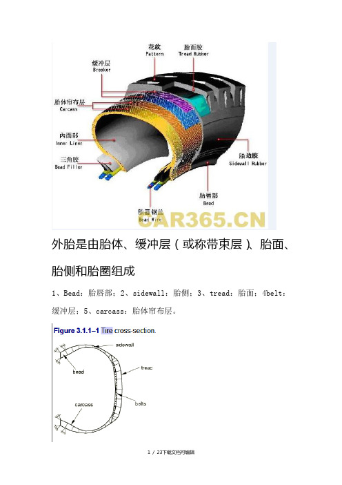
外胎是由胎体、缓冲层(或称带束层)、胎面、胎侧和胎圈组成1、Bead:胎唇部;2、sidewall:胎侧;3、tread:胎面;4belt:缓冲层;5、carcass:胎体帘布层。
3.1.8 Tread wear simulation using adaptive meshing in Abaqus/Standard3.1.8使用自适应网格在Abaqus/Standard中进行轮胎磨损仿真分析软件:Abaqus/Standard这个例子在Abaqus/Standard中使用自适应网格技术对稳态滚动的轮胎进行建模。
这次分析使用类似“Steady-state rolling analysis of a tire”Section 3.1.2来建立稳态滚动轮胎的接地印迹和状态。
接着,进行稳态传输分析来计算和推测持续分析步,在稳态过程中产生一个近似瞬态磨损解。
问题描述和建模轮胎描述和有限元建模和“Import of a steady-state rolling tire,”Section 3.1.6一样,但是有一些不一样,在这里需要指出。
由于这次分析的中心是轮胎磨损,所以胎面建模需要更加精细。
另外台面使用线性弹性材料模型来避免超弹性材料在网格自适应过程中不收敛。
图1所示的是轴对称175SR14轮胎的一半模型。
橡胶层用CGAX4和CGAX3单元建模。
加强层使用带有rebar层的SFMGAX1单元模拟。
橡胶层和加强层之间潜入单元约束。
橡胶层的弹性模量为6Mpa,泊松比为0.49。
剩下的轮胎部分用超弹性材料模型模拟。
多应变能使用系数C10=10^6,C01=0和D1=2*10^8。
用来模拟骨架纤维的刚性层和径向成0°,弹性模量为9.87Gpa。
压缩系数设置成受拉系数的百分之一。
名义应力应变数据用马洛超弹性模型定义材料本构关系。
Belt fibers材料的拉伸弹性模量为172.2Gpa。
压缩系数设置成拉伸系数的的百分之一。
Abaqus关于用户子程序(simwe)
Abaqus关于用户子程序(simwe)序,但可以调用用户自己编写的FORTRAN子程序和ABAQUS应用程序。
当用户编写FORTRAN子程序时,建议子程序名以K开头,以免和ABAQUS内部程序冲突。
2.当用户在用户子程序中利用OPEN打开外部文件时,要注意以下两点:一是设备号的选择是有限制的,只能取15-18和大于100的设备号,其余的都已被ABAQUS占用。
二是用户需提供外部文件的绝对路径而不是相对路径。
3.ABAQUS 应用程序必须由用户子程序调用。
当用到某个用户子程序时,用户所关心的主要有两方面:一是ABAQUS提供的用户子程序的接口参数。
有些参数是ABAQUS传到用户子程序中的,例如SUBROUTINE DLOAD中的KSTEP,KINC,COORDS;有些是需要用户自己定义的,例如F。
二是ABAQUS何时调用该用户子程序,对于不同的用户子程序ABAQUS调用的时间是不同的。
有些是在每个STEP的开始,有的是STEP结尾,有的是在每个INCREMENT的开始等等。
当ABAQUS调用用户子程序是,都会把当前的STEP和INCREMENT利用用户子程序的两个实参KSTEP和KINC传给用户子程序,用户可编个小程序把它们输出到外部文件中,这样对ABAQUS何时调用该用户子程序就会有更深的了解。
下面就选出几个常用的用户子程序和应用程序进行详细解释:一.SUBROUTINEDLOAD(F,KSTEP,KINC,TIME,NOEL,NPT,LAYER,KSPT,COORDS, JLTYP,SNAME)参数:1. F为用户定义的是每个积分点所作用的荷载的大小;2.KSTEP,KINC为ABAQUS传到用户子程序当前的STEP和INCREMENT值;3. TIME(1),TIME(2)为当前STEP TIME和INCREMENT TIME的值;4. NOEL,NPT为积分点所在单元的编号和积分点的编号;5. COORDS为当前积分点的坐标;6.除F外,所有参数的值都是ABAQUS传到用户子程序中的。
abaqus1用户材料子程序
19 ABAQUS用户材料子程序(UMAT)虽然ABAQUS为用户提供了大量的单元库和求解模型,使用户能够利用这些模型处理绝大多数的问题;但是现实世界毕竟十分复杂,ABAQUS不可能把所有可能出现的问题都包含进去。
所以ABAQUS提供了大量的用户子程序(User Subroutine)。
用户子程序允许用户在找不到合适模型的情况下自行定义符合自己问题的模型。
这些用户子程序涵盖了建模从载荷到单元的几乎各个部分。
ABAQUS为用户提供的这个接口,允许用户通过自定义的子程序定制ABAQUS,以实现特定的功能。
用户子程序具有以下的功能和特点:(1)如果ABAQUS的一些固有选项模型功能有限;用户子程序可以提高ABAQUS中这些选项的功能;(2)通常用户子程序是用FORTRAN语言的代码写成;(3)它可以以几种不同的方式包含在模型中;(4)由于它们没有存储在restart文件中,如果需要的话,可以在重新开始运行时修改它;(5)在某些情况下它可以利用ABAQUS允许的已有程序。
要在模型中包含用户子程序,可以利用ABAQUS执行程序,在abaqus执行程序中应用user选项指明包含这些子程序的FORTRAN源程序或者目标程序的名字。
提示:ABAQUS的输入文件除了可以通过ABAQUS/CAE的作业模块中提交运行外,还可以在ABAQUS Command窗口中输入ABAQUS执行程序直接运行:ABAQUS job=输入文件名 user=用户子程序的Fortran文件名ABAQUS/Standard和ABAQUS/Explicit都支持用户子程序功能,但是他们所支持的用户子程序种类不尽相同,读者在需要使用时请注意查询手册。
在接下来的最后两章里,我们将讨论两种常用的用户子程序——用户材料子程序和用户单元子程序。
本章将通过在ABAQUS/Standard中创建Johnson-Cook的材料模型,对编写Standard 的用户材料子程序UMAT进行一个简单介绍。