ABAQUS帮助文档
ABAQUS帮助范例中文索引
帮助文档ABAQUS Example Problems Menual1.静态应力/位移分析1.1.静态与准静态应力分析1.1.1.螺栓结合型管法兰连接的轴对称分析1.1.2.薄壁机械肘在平面弯曲与内部压力下的弹塑性失效1.1.3.线弹性管线在平面弯曲下的参数研究1.1.4.橡胶海绵在圆形凸模下的变形分析1.1.5.混泥土板的失效1.1.6.有接缝的石坡稳定性研究1.1.7.锯齿状梁在循环载荷下的响应1.1.8.静水力学流体单元:空气弹簧模型1.1.9.管连接中的壳-固体子模型与壳-固体耦合的建立1.1.10.无应力单元的再激活1.1.11.黏弹性轴衬的动载响应1.1.12.厚板的凹入响应1.1.13.叠层复合板的损害和失效1.1.14.汽车密封套分析1.1.15.通风道接缝密封的压力渗透分析1.1.16.震动缓冲器的橡胶/海绵成分的自接触分析1.1.17.橡胶垫圈的橡胶/海绵成分的自接触分析1.1.18.堆叠金属片装配中的子模型分析1.1.19.螺纹连接的轴对称分析1.1.20.周期热-机械载荷下的汽缸盖的直接循环分析1.1.21.材料(沙产品)在油井中的侵蚀分析1.1.22.压力容器盖的子模型应力分析1.1.23.模拟游艇船体中复合涂覆层的应用1.2.屈曲与失效分析1.2.1.圆拱的完全弯曲分析1.2.2. 层压复合壳中带圆孔圆柱形面的屈曲分析1.2.3.点焊圆柱的屈曲分析1.2.4. K型结构的弹塑性分析1.2.5. 不稳定问题:压缩载荷下的加强板分析1.2.6.缺陷敏感柱型壳的屈曲分析1.3. 成形分析1.3.1. 圆柱形坯料墩粗:利用网格对网格方案配置与自适应网格的准静态分析1.3.2. 矩形方盒的超塑性成型1.3.3. 球形凸模的薄板拉伸1.3.4. 圆柱杯的深拉伸1.3.5. 考虑摩擦热产生的圆柱形棒材的挤压成形分析1.3.6. 厚板轧制成形分析1.3.7. 圆柱杯的轴对称成形分析1.3.8. 杯/槽成形分析1.3.9. 正弦曲线形凹模锻造1.3.10. 多重复合凹模锻造1.3.11. 平滑辊成形中的瞬态与稳态分析1.3.12. 型钢扎制成形分析1.3.13. 环扎成形分析1.3.14. 轴对称挤压成形中的瞬态与稳态分析1.3.15. 两步成形仿真1.3.16. 圆柱形坯料墩粗:热-位移耦合与隔热分析1.3.17. 金属板热成形中的不稳定静态问题分析1.4. 破裂与损伤1.4.1. 平板局部破裂分析:弹性线弹簧模拟1.4.2. 线弹性无限半空间中的锥裂纹围道积分1.4.3. 带局部轴向裂纹有限长度圆筒的弹塑性线弹簧模拟1.4.4. 三点弯曲试件的裂纹扩展1.4.5. 压力下刚性表面的松解工艺分析1.4.6. 钝角槽光纤金属绝缘板的失效分析1.5. 输入分析1.5.1. 二维拉伸弯曲的回弹1.5.2. 方形盒的深拉伸2. 动态应力/位移分析2.1. 动态应力分析2.1.1. 有局部非弹性失效结构的非线性动态分析2.1.2. Detroit Edison管滑轮试验2.1.3. 刚性抛丸对板的变化及影响2.1.4. 侵蚀抛丸对板的变化及影响2.1.5. 网球拍与球2.1.6. 变厚度燃料水槽壳的受压分析2.1.7. 汽车悬架模拟2.1.8. 管塞爆炸2.1.9. 常规接触的膝垫效应2.1.10. 常规接触的压接成形2.1.11. 常规接触的堆块失稳2.1.12. 带海绵效应限幅器的木桶坠落2.1.13. 铜杆的斜碰2.1.14. 带挡板木桶中的流体晃动2.1.15. 混泥土重力坝的地震分析2.1.16. 准静态或动载下薄壁铝挤压成形中的逐步损坏分析2.2. 基于模态的动态分析2.2.1.利用子结构和循环对称的旋转风扇分析2.2.2.Indian Point反应堆给水线的线性分析2.2.3. 三维框架建筑的感应波谱2.2.4. 使用平行Lanczos本征求解器结构的特征值分析2.2.5. 制动噪声分析2.2.6. 使用剩余模态的天线结构的动态分析2.2.7. 白车身模型的恒定动态分析2.3.联合仿真分析2.3.1. 充气门密封的关闭模拟。
Abaqus User Subroutines Reference Guide 用户材料子程序帮助文档
1.1.41 UMATUser subroutine to define a material's mechanical behavior.Product: Abaqus/StandardWarning: The use of this subroutine generally requires considerable expertise. Y ou arecautioned that the implementation of any realistic constitutive model requires extensivedevelopment and testing. Initial testing on a single-element model with prescribedtraction loading is strongly recommended.References“User-defined mechanical material behavior,” Section 26.7.1 of the Abaqus Analysis User's Guide“User-defined thermal material behavior,” Section 26.7.2 of the Abaqus Analysis User's Guide*USER MA TERIAL“S D V I N I,” Section 4.1.11 of the Abaqus V erification Guide“U M A T and U H Y P E R,” Section 4.1.21 of the Abaqus V erification GuideOv erv iewUser subroutine U M A T:can be used to define the mechanical constitutive behavior of a material;will be called at all material calculation points of elements for which the material definition includes auser-defined material behavior;can be used with any procedure that includes mechanical behavior;can use solution-dependent state variables;must update the stresses and solution-dependent state variables to their values at the end of theincrement for which it is called;must provide the material Jacobian matrix, , for the mechanical constitutive model;can be used in conjunction with user subroutine U S D F L D to redefine any field variables before they are passed in; andis described further in “User-defined mechanical material behavior,” Section 26.7.1 of the AbaqusAnalysis User's Guide.Storage of stress and strain componentsIn the stress and strain arrays and in the matrices D D S D D E, D D S D D T, and D R P L D E, direct components are stored first, followed by shear components. There are N D I direct and N S H R engineering shear components. The order of the components is defined in “Conventions,” Section 1.2.2 of the Abaqus Analysis User's Guide. Since the number of active stress and strain components varies between element types, the routine must be coded toprovide for all element types with which it will be used.Defining local orientationsIf a local orientation (“Orientations,” Section 2.2.5 of the Abaqus Analysis User's Guide) is used at the same point as user subroutine U M A T, the stress and strain components will be in the local orientation; and, in the case of finite-strain analysis, the basis system in which stress and strain components are stored rotates with the material.StabilityY ou should ensure that the integration scheme coded in this routine is stable—no direct provision is made to include a stability limit in the time stepping scheme based on the calculations in U M A T.Convergence rateD D S D DE and—for coupled temperature-displacement and coupled thermal-electrical-structural analyses—D D S D D T, D R P L D E, and D R P L D T must be defined accurately if rapid convergence of the overall Newton scheme is to be achieved. In most cases the accuracy of this definition is the most important factor governing the convergence rate. Since nonsymmetric equation solution is as much as four times as expensive as the corresponding symmetric system, if the constitutive Jacobian (D D S D D E) is only slightly nonsymmetric (for example, a frictional material with a small friction angle), it may be less expensive computationally to use a symmetric approximation and accept a slower convergence rate.An incorrect definition of the material Jacobian affects only the convergence rate; the results (if obtained) are unaffected.Special considerations for various element typesThere are several special considerations that need to be noted.A v ailability of deformation gradientThe deformation gradient is available for solid (continuum) elements, membranes, and finite-strain shells(S3/S3R, S4, S4R, SAXs, and SAXAs). It is not available for beams or small-strain shells. It is stored as a 3× 3 matrix with component equivalence D F G R D0(I,J). For fully integrated first-order isoparametric elements (4-node quadrilaterals in two dimensions and 8-node hexahedra in three dimensions) the selectively reduced integration technique is used (also known as the technique). Thus, a modified deformation gradientis passed into user subroutine U M A T. For more details, see “Solid isoparametric quadrilaterals and hexahedra,”Section 3.2.4 of the Abaqus Theory Guide.Beams and shells that calculate transv erse shear energyIf user subroutine U M A T is used to describe the material of beams or shells that calculate transverse shear energy, you must specify the transverse shear stiffness as part of the beam or shell section definition to define the transverse shear behavior. See “Shell section behavior,” Section 29.6.4 of the Abaqus Analysis User's Guide, and “Choosing a beam element,” Section 29.3.3 of the Abaqus Analysis User's Guide, for informationon specifying this stiffness.Open-section beam elementsWhen user subroutine U M A T is used to describe the material response of beams with open sections (for example, an I-section), the torsional stiffness is obtained aswhere J is the torsional constant, A is the section area, k is a shear factor, and is the user-specified transverse shear stiffness (see “Transverse shear stiffness definition” in “Choosing a beam element,” Section29.3.3 of the Abaqus Analysis User's Guide).E lements w ith hourglassing modesIf this capability is used to describe the material of elements with hourglassing modes, you must define the hourglass stiffness factor for hourglass control based on the total stiffness approach as part of the element section definition. The hourglass stiffness factor is not required for enhanced hourglass control, but you can define a scaling factor for the stiffness associated with the drill degree of freedom (rotation about the surface normal). See “Section controls,” Section 27.1.4 of the Abaqus Analysis User's Guide, for information on specifying the stiffness factor.Pipe-soil interaction elementsThe constitutive behavior of the pipe-soil interaction elements (see “Pipe-soil interaction elements,” Section 32.12.1 of the Abaqus Analysis User's Guide) is defined by the force per unit length caused by relative displacement between two edges of the element. The relative-displacements are available as “strains” (S T R A N and D S T R A N). The corresponding forces per unit length must be defined in the S T R E S S array. The Jacobian matrix defines the variation of force per unit length with respect to relative displacement.For two-dimensional elements two in-plane components of “stress” and “strain” exist (N T E N S=N D I=2, andN S H R=0). For three-dimensional elements three components of “stress” and “strain” exist (N T E N S=N D I=3, and N S H R=0).Large volume changes with geometric nonlinearityIf the material model allows large volume changes and geometric nonlinearity is considered, the exact definition of the consistent Jacobian should be used to ensure rapid convergence. These conditions are most commonly encountered when considering either large elastic strains or pressure-dependent plasticity. In the former case, total-form constitutive equations relating the Cauchy stress to the deformation gradient are commonly used; in the latter case, rate-form constitutive laws are generally used.For total-form constitutive laws, the exact consistent Jacobian is defined through the variation in Kirchhoff stress:Here, J is the determinant of the deformation gradient, is the Cauchy stress, is the virtual rate of deformation, and is the virtual spin tensor, defined asFor rate-form constitutive laws, the exact consistent Jacobian is given byUse with incompressible elastic materialsFor user-defined incompressible elastic materials, user subroutine U H Y P E R should be used rather than user subroutine U M A T. In U M A T incompressible materials must be modeled via a penalty method; that is, you must ensure that a finite bulk modulus is used. The bulk modulus should be large enough to model incompressibility sufficiently but small enough to avoid loss of precision. As a general guideline, the bulk modulus should be about – times the shear modulus. The tangent bulk modulus can be calculated fromIf a hybrid element is used with user subroutine U M A T, Abaqus/Standard will replace the pressure stress calculated from your definition of S T R E S S with that derived from the Lagrange multiplier and will modify the Jacobian appropriately.For incompressible pressure-sensitive materials the element choice is particularly important when using user subroutine U M A T. In particular, first-order wedge elements should be avoided. For these elements the technique is not used to alter the deformation gradient that is passed into user subroutine U M A T, which increases the risk of volumetric locking.Increments for which only the Jacobian can be definedAbaqus/Standard passes zero strain increments into user subroutine U M A T to start the first increment of all the steps and all increments of steps for which you have suppressed extrapolation (see “Defining an analysis,”Section 6.1.2 of the Abaqus Analysis User's Guide). In this case you can define only the Jacobian (D D S D D E).Utility routinesSeveral utility routines may help in coding user subroutine U M A T. Their functions include determining stress invariants for a stress tensor and calculating principal values and directions for stress or strain tensors. These utility routines are discussed in detail in “Obtaining stress invariants, principal stress/strain values and directions, and rotating tensors in an Abaqus/Standard analysis,” Section 2.1.11.U ser subroutine interfaceS U B R O U T I N E U M A T(S T R E S S,S T A T E V,D D S D D E,S S E,S P D,S C D,1R P L,D D S D D T,D R P L D E,D R P L D T,2S T R A N,D S T R A N,T I M E,D T I M E,T E M P,D T E M P,P R E D E F,D P R E D,C M N A M E,3N D I,N S H R,N T E N S,N S T A T V,P R O P S,N P R O P S,C O O R D S,D R O T,P N E W D T,4C E L E N T,D F G R D0,D F G R D1,N O E L,N P T,L A Y E R,K S P T,K S T E P,K I N C)CI N C L U D E'A B A_P A R A M.I N C'C H A R A C T E R*80C M N A M ED I ME N S I O N S T R E S S(N T E N S),S T A T E V(N S T A T V),1D D S D D E(N T E N S,N T E N S),D D S D D T(N T E N S),D R P L D E(N T E N S),2S T R A N(N T E N S),D S T R A N(N T E N S),T I M E(2),P R E D E F(1),D P R E D(1),3P R O P S(N P R O P S),C O O R D S(3),D R O T(3,3),D F G R D0(3,3),D F G R D1(3,3)user coding to define D D S D D E,S T R E S S,S T A T E V,S S E,S P D,S C Dand, if necessary,R P L,D D S D D T,D R P L D E,D R P L D T,P N E W D TR E T U R NE N DV ariables to be definedIn all situationsD D S D D E(N TE N S,N T E N S)Jacobian matrix of the constitutive model, , where are the stress increments and are the strain increments. D D S D D E(I,J) defines the change in the I th stress component at the end of the time increment caused by an infinitesimal perturbation of the J th component of the strain increment array.Unless you invoke the unsymmetric equation solution capability for the user-defined material,Abaqus/Standard will use only the symmetric part of D D S D D E. The symmetric part of the matrix iscalculated by taking one half the sum of the matrix and its transpose.S T R E S S(N T E N S)This array is passed in as the stress tensor at the beginning of the increment and must be updated in this routine to be the stress tensor at the end of the increment. If you specified initial stresses (“Initial conditions in Abaqus/Standard and Abaqus/Explicit,” Section 34.2.1 of the Abaqus Analysis User's Guide), this array will contain the initial stresses at the start of the analysis. The size of this array depends on the value of N T E N S as defined below. In finite-strain problems the stress tensor has already been rotated to account for rigid body motion in the increment before U M A T is called, so that only the corotational part of the stress integration should be done in U M A T. The measure of stress used is “true” (Cauchy) stress.S T A T E V(N S T A T V)An array containing the solution-dependent state variables. These are passed in as the values at thebeginning of the increment unless they are updated in user subroutines U S D F L D or U E X P A N, in which case the updated values are passed in. In all cases S T A T E V must be returned as the values at the end of the increment. The size of the array is defined as described in “Allocating space” in “User subroutines:overview,” Section 18.1.1 of the Abaqus Analysis User's Guide.In finite-strain problems any vector-valued or tensor-valued state variables must be rotated to account for rigid body motion of the material, in addition to any update in the values associated with constitutivebehavior. The rotation increment matrix, D R O T, is provided for this purpose.S S E,S P D,S C DSpecific elastic strain energy, plastic dissipation, and “creep” dissipation, respectively. These are passed in as the values at the start of the increment and should be updated to the corresponding specific energy values at the end of the increment. They have no effect on the solution, except that they are used forenergy output.Only in a fully coupled thermal-stress or a coupled thermal-electrical-structural analysisR P LV olumetric heat generation per unit time at the end of the increment caused by mechanical working of the material.D D S D D T(N TE N S)V ariation of the stress increments with respect to the temperature.D R P L D E(N TE N S)V ariation of R P L with respect to the strain increments.D R P L D TV ariation of R P L with respect to the temperature.Only in a geostatic stress procedure or a coupled pore fluid diffusion/stress analysis for pore pressure cohesive elementsR P LR P L is used to indicate whether or not a cohesive element is open to the tangential flow of pore fluid. Set R P L equal to 0 if there is no tangential flow; otherwise, assign a nonzero value to R P L if an element is open.Once opened, a cohesive element will remain open to the fluid flow.V ariable that can be updatedP N E W D TRatio of suggested new time increment to the time increment being used (D T I M E, see discussion later in this section). This variable allows you to provide input to the automatic time incrementation algorithms in Abaqus/Standard (if automatic time incrementation is chosen). For a quasi-static procedure the automatic time stepping that Abaqus/Standard uses, which is based on techniques for integrating standard creep laws (see “Quasi-static analysis,” Section 6.2.5 of the Abaqus Analysis User's Guide), cannot becontrolled from within the U M A T subroutine.P N E W D T is set to a large value before each call to U M A T.If P N E W D T is redefined to be less than 1.0, Abaqus/Standard must abandon the time increment andattempt it again with a smaller time increment. The suggested new time increment provided to theautomatic time integration algorithms is P N E W D T × D T I M E, where the P N E W D T used is the minimum value for all calls to user subroutines that allow redefinition of P N E W D T for this iteration.If P N E W D T is given a value that is greater than 1.0 for all calls to user subroutines for this iteration and the increment converges in this iteration, Abaqus/Standard may increase the time increment. The suggestednew time increment provided to the automatic time integration algorithms is P N E W D T × D T I M E, where the P N E W D T used is the minimum value for all calls to user subroutines for this iteration.If automatic time incrementation is not selected in the analysis procedure, values of P N E W D T that aregreater than 1.0 will be ignored and values of P N E W D T that are less than 1.0 will cause the job to terminate. V ariables passed in for informationS T R A N(N T E N S)An array containing the total strains at the beginning of the increment. If thermal expansion is included in the same material definition, the strains passed into U M A T are the mechanical strains only (that is, thethermal strains computed based upon the thermal expansion coefficient have been subtracted from the total strains). These strains are available for output as the “elastic” strains.In finite-strain problems the strain components have been rotated to account for rigid body motion in the increment before U M A T is called and are approximations to logarithmic strain.D S T R A N(N TE N S)Array of strain increments. If thermal expansion is included in the same material definition, these are the mechanical strain increments (the total strain increments minus the thermal strain increments).T I M E(1)V alue of step time at the beginning of the current increment or frequency.T I M E(2)V alue of total time at the beginning of the current increment.D T I M ETime increment.T E M PTemperature at the start of the increment.D TE M PIncrement of temperature.P R E D E FArray of interpolated values of predefined field variables at this point at the start of the increment, based on the values read in at the nodes.D P RE DArray of increments of predefined field variables.C M N A M EUser-defined material name, left justified. Some internal material models are given names starting with the “ABQ_” character string. To avoid conflict, you should not use “ABQ_” as the leading string for C M N A M E. N D INumber of direct stress components at this point.N S H RNumber of engineering shear stress components at this point.N T E N SSize of the stress or strain component array (N D I + N S H R).N S T A T VNumber of solution-dependent state variables that are associated with this material type (defined asdescribed in “Allocating space” in “User subroutines: overview,” Section 18.1.1 of the Abaqus Analysis User's Guide).P R O P S(N P R O P S)User-specified array of material constants associated with this user material.N P R O P SUser-defined number of material constants associated with this user material.C O O RD SAn array containing the coordinates of this point. These are the current coordinates if geometricnonlinearity is accounted for during the step (see “Defining an analysis,” Section 6.1.2 of the Abaqus Analysis User's Guide); otherwise, the array contains the original coordinates of the point.D R O T(3,3)Rotation increment matrix. This matrix represents the increment of rigid body rotation of the basis system in which the components of stress (S T R E S S) and strain (S T R A N) are stored. It is provided so that vector-or tensor-valued state variables can be rotated appropriately in this subroutine: stress and straincomponents are already rotated by this amount before U M A T is called. This matrix is passed in as a unit matrix for small-displacement analysis and for large-displacement analysis if the basis system for thematerial point rotates with the material (as in a shell element or when a local orientation is used).C E L E N TCharacteristic element length, which is a typical length of a line across an element for a first-order element;it is half of the same typical length for a second-order element. For beams and trusses it is a characteristic length along the element axis. For membranes and shells it is a characteristic length in the referencesurface. For axisymmetric elements it is a characteristic length in the plane only. For cohesiveelements it is equal to the constitutive thickness.D F G R D0(3,3)Array containing the deformation gradient at the beginning of the increment. If a local orientation is defined at the material point, the deformation gradient components are expressed in the local coordinate system defined by the orientation at the beginning of the increment. For a discussion regarding the availability of the deformation gradient for various element types, see “Availability of deformation gradient.”D F G R D1(3,3)Array containing the deformation gradient at the end of the increment. If a local orientation is defined at the material point, the deformation gradient components are expressed in the local coordinate system defined by the orientation. This array is set to the identity matrix if nonlinear geometric effects are not included in the step definition associated with this increment. For a discussion regarding the availability of thedeformation gradient for various element types, see “Availability of deformation gradient.”N O E LElement number.N P TIntegration point number.L A Y E RLayer number (for composite shells and layered solids).K S P TSection point number within the current layer.K S T E PStep number.K I N CIncrement number.Example: Using more than one user-defined mechanical material modelTo use more than one user-defined mechanical material model, the variable C M N A M E can be tested for different material names inside user subroutine U M A T as illustrated below:I F(C M N A M E(1:4).E Q.'M A T1')T H E NC A L L U M A T_M A T1(argument_list)E L S E I F(C M N A M E(1:4).E Q.'M A T2')T H E NC A L L U M A T_M A T2(argument_list)E N D I FU M A T_M A T1 and U M A T_M A T2 are the actual user material subroutines containing the constitutive material models for each material M A T1 and M A T2, respectively. Subroutine U M A T merely acts as a directory here. The argument list may be the same as that used in subroutine U M A T.Example: Simple linear viscoelastic materialAs a simple example of the coding of user subroutine U M A T, consider the linear, viscoelastic model shown in Figure 1.1.41–1. Although this is not a very useful model for real materials, it serves to illustrate how to code the routine.Figure 1.1.41–1 Simple linear viscoelastic model.The behavior of the one-dimensional model shown in the figure iswhere and are the time rates of change of stress and strain. This can be generalized for small straining of an isotropic solid asandwhereand , , , , and are material constants ( and are the Lamé constants).A simple, stable integration operator for this equation is the central difference operator:where f is some function, is its value at the beginning of the increment, is the change in the function over the increment, and is the time increment.Applying this to the rate constitutive equations above givesandso that the Jacobian matrix has the termsandThe total change in specific energy in an increment for this material iswhile the change in specific elastic strain energy iswhere D is the elasticity matrix:No state variables are needed for this material, so the allocation of space for them is not necessary. In a morerealistic case a set of parallel models of this type might be used, and the stress components in each model might be stored as state variables.For our simple case a user material definition can be used to read in the five constants in the order , , , , and so thatThe routine can then be coded as follows:S U B R O U T I N E U M A T(S T R E S S,S T A T E V,D D S D D E,S S E,S P D,S C D,1R P L,D D S D D T,D R P L D E,D R P L D T,2S T R A N,D S T R A N,T I M E,D T I M E,T E M P,D T E M P,P R E D E F,D P R E D,C M N A M E,3N D I,N S H R,N T E N S,N S T A T V,P R O P S,N P R O P S,C O O R D S,D R O T,P N E W D T,4C E L E N T,D F G R D0,D F G R D1,N O E L,N P T,L A Y E R,K S P T,K S T E P,K I N C)CI N C L U D E'A B A_P A R A M.I N C'CC H A R A C T E R*80C M N A M ED I ME N S I O N S T R E S S(N T E N S),S T A T E V(N S T A T V),1D D S D D E(N T E N S,N T E N S),2D D S D D T(N T E N S),D R P L D E(N T E N S),3S T R A N(N T E N S),D S T R A N(N T E N S),T I M E(2),P R E D E F(1),D P R E D(1),4P R O P S(N P R O P S),C O O R D S(3),D R O T(3,3),D F G R D0(3,3),D F G R D1(3,3)D I ME N S I O N D S T R E S(6),D(3,3)CC E V A L U A T E N E W S T R E S S T E N S O RCE V=0.D E V=0.D O K1=1,N D IE V=E V+S T R A N(K1)D E V=D E V+D S T R A N(K1)E N D D OCT E R M1=.5*D T I M E+P R O P S(5)T E R M1I=1./T E R M1T E R M2=(.5*D T I M E*P R O P S(1)+P R O P S(3))*T E R M1I*D E VT E R M3=(D T I M E*P R O P S(2)+2.*P R O P S(4))*T E R M1ICD O K1=1,N D ID S T RE S(K1)=T E R M2+T E R M3*D S T R A N(K1)1+D T I M E*T E R M1I*(P R O P S(1)*E V2+2.*P R O P S(2)*S T R A N(K1)-S T R E S S(K1))S T R E S S(K1)=S T R E S S(K1)+D S T R E S(K1)E N D D OCT E R M2=(.5*D T I M E*P R O P S(2)+P R O P S(4))*T E R M1II1=N D ID O K1=1,N S H RI1=I1+1D S T RE S(I1)=T E R M2*D S T R A N(I1)+1D T I M E*T E R M1I*(P R O P S(2)*S T R A N(I1)-S T R E S S(I1)) S T R E S S(I1)=S T R E S S(I1)+D S T R E S(I1)E N D D OCC C R E A T E N E W J A C O B I A NCT E R M2=(D T I M E*(.5*P R O P S(1)+P R O P S(2))+P R O P S(3)+12.*P R O P S(4))*T E R M1IT E R M3=(.5*D T I M E*P R O P S(1)+P R O P S(3))*T E R M1ID O K1=1,N TE N SD O K2=1,N TE N SD D S D D E(K2,K1)=0.E N D D OE N D D OCD O K1=1,N D ID D S D D E(K1,K1)=TE R M2E N D D OCD O K1=2,N D IN2=K1–1D O K2=1,N2D D S D D E(K2,K1)=TE R M3D D S D D E(K1,K2)=TE R M3E N D D OE N D D OT E R M2=(.5*D T I M E*P R O P S(2)+P R O P S(4))*T E R M1II1=N D ID O K1=1,N S H RI1=I1+1D D S D D E(I1,I1)=TE R M2E N D D OCC T O T A L C H A N G E I N S P E C I F I C E N E R G YCT D E=0.D O K1=1,N TE N ST D E=T D E+(S T R E S S(K1)-.5*D S T R E S(K1))*D S T R A N(K1)E N D D OCC C H A N G E I N S P E C I F I C E L A S T I C S T R A I N E N E R G YCT E R M1=P R O P S(1)+2.*P R O P S(2)D O K1=1,N D ID(K1,K1)=T E R M1E N D D OD O K1=2,N D IN2=K1-1D O K2=1,N2D(K1,K2)=P R O P S(1)D(K2,K1)=P R O P S(1)E N D D OE N D D OD E E=0.D O K1=1,N D IT E R M1=0.T E R M2=0.D O K2=1,N D IT E R M1=T E R M1+D(K1,K2)*S T R A N(K2)T E R M2=T E R M2+D(K1,K2)*D S T R A N(K2)E N D D OD E E=D E E+(T E R M1+.5*T E R M2)*D S T R A N(K1)E N D D OI1=N D ID O K1=1,N S H RI1=I1+1D E E=D E E+P R O P S(2)*(S T R A N(I1)+.5*D S T R A N(I1))*D S T R A N(I1)E N D D OS S E=S S E+D E ES C D=S C D+T D E– D E ER E T U R NE N D。
ABAQUS帮助文档

初始损伤对应于材料开场退化,当应力或应变满足于定义的初始临界损伤准则,则此时退化开场。
Abaqus 的Damage for traction separation laws 中包括:Quade Damage、Ma*e Damage、Quads Damage、Ma*s Damage、Ma*pe Damage、Ma*ps Damage 六种初始损伤准则,其中前四种用于一般复合材料分层模拟,后两种主要是在扩展有限元法模拟不连续体〔比方crack 问题〕问题时使用。
前四种对应于界面单元的含义如下: Ma*e Damage 最大名义应变准则: Ma*s Damage 最大名义应力准则: Quads Damage 二次名义应变准则: Quade Damage 二次名义应力准则最大主应力和最大主应变没有特定的联系,不同材料适用不同准则就像强度理论有最大应力理论和最大应变理论一样~ABAQUS帮助文档10.7.1 Modeling discontinuities as an enriched feature using the e*tended finite element method 看看里面有没有你想要的Defining damage evolution based on energy dissipated during the damage process根据损伤过程中消耗的能量定义损伤演变You can specify the fracture energy per unit area,, to be dissipated during the damage process directly.您可以指定每单位面积的断裂能量,在损坏过程中直接消散。
Instantaneous failure will occur if is specified as 0.瞬间失效将发生However, this choice is not remended and should be used with care because it causes a sudden drop in the stress at the material point that can lead to dynamic instabilities.但是,不推荐这种选择,应慎重使用,因为它会导致材料点的应力突然下降,从而导致动态不稳定。
abaqus子结构帮助文档
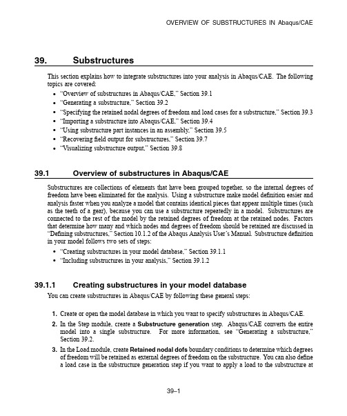
OVERVIEW OF SUBSTRUCTURES IN Abaqus/CAE39.SubstructuresThis section explains how to integrate substructures into your analysis in Abaqus/CAE.The following topics are covered:•“Overview of substructures in Abaqus/CAE,”Section39.1•“Generating a substructure,”Section39.2•“Specifying the retained nodal degrees of freedom and load cases for a substructure,”Section39.3•“Importing a substructure into Abaqus/CAE,”Section39.4•“Using substructure part instances in an assembly,”Section39.5•“Recoveringfield output for substructures,”Section39.7•“Visualizing substructure output,”Section39.839.1Overview of substructures in Abaqus/CAESubstructures are collections of elements that have been grouped together,so the internal degrees of freedom have been eliminated for the ing a substructure make model definition easier and analysis faster when you analyze a model that contains identical pieces that appear multiple times(such as the teeth of a gear),because you can use a substructure repeatedly in a model.Substructures are connected to the rest of the model by the retained degrees of freedom at the retained nodes.Factors that determine how many and which nodes and degrees of freedom should be retained are discussed in “Defining substructures,”Section10.1.2of the Abaqus Analysis User’s Manual.Substructure definition in your model follows two sets of steps:•“Creating substructures in your model database,”Section39.1.1•“Including substructures in your analysis,”Section39.1.239.1.1Creating substructures in your model databaseYou can create substructures in Abaqus/CAE by following these general steps:1.Create or open the model database in which you want to specify substructures in Abaqus/CAE.2.In the Step module,create a Substructure generation step.Abaqus/CAE converts the entiremodel into a single substructure.For more information,see“Generating a substructure,”Section39.2.3.In the Load module,create Retained nodal dofs boundary conditions to determine which degreesof freedom will be retained as external degrees of freedom on the substructure.You can also definea load case in the substructure generation step if you want to apply a load to the substructure atGENERA TING A SUBSTRUCTUREa location other than its retained degrees of freedom.For more information,see“Specifying theretained nodal degrees of freedom and load cases for a substructure,”Section39.3.4.In the Job module,create a new job and submit the analysis.When you perform an analysis of an assembly that includes substructure data,Abaqus/CAE creates separate output databases for the results of each substructure part instance and does not include the results from the substructure part instances in the output database for the assembly.The Visualization module provides tools that enable you to integrate the results from the substructure components back into the results from the assembly;for more information,see“Visualizing substructure output,”Section39.8.39.1.2Including substructures in your analysisSubstructure usage should be performed in a different model than substructure generation.You can include substructures in your analysis in Abaqus/CAE by following these general steps:1.Import each substructure that you want to use in your model database from the corresponding.simfile.For more information,see“Importing a substructure into Abaqus/CAE,”Section39.4,in the online HTML version of this manual.2.In the Assembly module,instance each substructure part that you want to add to the assembly,andposition the substructure part instances in the desired locations in the assembly.“Using substructure part instances in an assembly,”Section39.5,explains the capabilities and limitations of substructure part instances.3.In the Load module,activate substructure load cases by creating a Substructure load definition.For more information,see“Activating load cases during substructure usage,”Section39.6.4.In the Step module,create afield output request with Substructure as the Domain,then select thesubstructure sets for which you want to recoverfield data.For more information,see“Recovering field output for substructures,”Section39.7.5.In the Interaction module,apply constraints to attach the substructure part instance to the rest of theassembly.39.2Generating a substructureThefirst step in substructure definition is the addition of a Substructure generate step in your analysis.The substructure generation step enables you to create a substructure in your model database and,if desired,specify substructure-related options such as the writing of the recovery matrix,stiffness matrix, mass matrix,and load case vectors to afile.These options are described later in this section.A single analysis can include multiple substructure generate steps,and Abaqus/CAE createscorresponding output databasefiles for each step.Multiple preloading steps can precede everySPECIFYING THE RETAINED NODAL DEGREES OF FREEDOM AND LOADCASES FOR A SUBSTRUCTURE substructure generation step in your analysis.If you want to specify retained eigenmodes forsubstructure generation,you must also include a frequency extraction step in the analysis.Substructure identifierYou must specify a unique identifier for each substructure you create.Substructure identifiers must begin with the letter Z followed by a number that cannot exceed999.Recovery optionsYou can recover thefield output data for a substructure during the usage-level analysis,but you must specify the recovery region during substructure generation.Substructure recovery can be performed only on the sets included in the recovery region.You can specify that recovery be performed on the whole model or for an individual node set or element set.While performing the substructure recovery in the usage model,Abaqus/CAE must have access to the substructure’s.mdl,.prt, .stt,and.supfiles.For more information about thesefile types,see“Defining substructures,”Section10.1.2of the Abaqus Analysis User’s Manual.Generation optionsYou can control several aspects of the substructure generation process,including calculation of gravity load vectors,evaluation of frequency-dependent material properties,and generation of a reduced mass matrix,reduced structural damping matrix,and viscous damping matrix.Retained eigenmodesYou can specify retained eigenmodes for generation of a coupled acoustic-structural substructure.When you choose to specify retained eigenmodes,Abaqus/CAE enables you to specify eigenmodes by mode range or by frequency range.DampingYou can specify several global damping controls and substructure damping controls.For global damping you can choose to apply damping settings to acoustic or mechanical options;for substructure damping you can specify separate controls for viscous and structural damping. 39.3Specifying the retained nodal degrees of freedom and load casesfor a substructureAfter you defined the substructure generation step or steps for your analysis,you must define a Retained nodal dofs boundary condition for a substructure.The retained degrees of freedom for a substructure node are the degrees of freedom that are external and are available for use in the analysis;all other degrees of freedom for the specified node are assumed to be internal to the substructure and do not factor into the analysis.When you import a substructure from this analysis into a model for substructure usage, Abaqus/CAE displays these nodes as light blue crosses,which enables you to pick them easily from a part instance or assembly.ACTIVA TING LOAD CASES DURING SUBSTRUCTURE USAGEIf you want to apply a load to the substructure at a location other than its retained degrees of freedom, you can define a load case in the substructure generation step.39.4Importing a substructure into Abaqus/CAEYou can include substructure definitions in a model database and begin to use them for modeling by importing the substructures as new part definitions.Substructure data are available in.simfiles, and the substructure identifier is included in thefile name;for example,in an analysis in which the substructure is named FAN and the substructure identifier is Z400,the substructure databasefile is named FAN_Z400.sim.The.simfile from which you import a substructure must reside in the same directory as the supporting Abaqusfiles to which the.sim database refers;these supportingfiles may include data in the formats.prt,.mdl,.stt,or.sup.Substructure import also requires an output database(.odb)file for mesh display.39.5Using substructure part instances in an assemblyOnce you import substructure parts into your model database,you can add them to your assembly by instancing them in the same manner you would for any part.Substructure part instances are displayed in a translucent color in the viewport.You can move and apply constraints to substructure part instances;however,substructure part instances have the following modeling limitations:•You cannot assign sections to a substructure part instance.•You cannot apply attributes to a substructure part instance.•Substructure part instances are not eligible for definition of contact pairs.•Gravity loads are the only load definition that can be applied to substructure part instances. 39.6Activating load cases during substructure usageThe Substructure load definition enables you to activate the substructure load cases that are specified during the substructure generation step.As you activate a load case,you can scale its load definitions or apply an amplitude to them.VISUALIZING SUBSTRUCTURE OUTPUT39.7Recovering field output for substructuresYou can specify that Abaqus/CAE writefield output data for one or more substructure sets in your analysis.From thefield output editor,select Substructure from the Domainfield,then click to open the Select Substructure Sets dialog box.This dialog box lists only the substructure sets that were defined while generating the substructure.You cannot recover data for sets that you define on substructure part instances in Abaqus/CAE.39.8Visualizing substructure outputAbaqus/CAE creates separate output database(.odb)files for each substructure part instance used in the analysis,so you must perform some additional steps if you want to display substructure results in context with the rest of the assembly.The Visualization module provides the following tools that enable you to incorporate substructure results into the rest of the model:•You can use an overlay plot to display plots of substructure data in the same viewport as a plot of the rest of the assembly.•You can use the Combine ODBs plug-in to combine the data in one or more substructure output databasefiles with the data from the rest of the assembly.。
Abaqus帮助文档整理汇总
feature)组成,每一个部分至少有一个基
base feature),特征体可以是所创建的实体,如挤压体、
.首先建立“部件”
1)根据实际模型的尺寸决定部件的近似尺寸,进入绘图区。绘图
edit菜
sketcher options选项里调整。
(比如奇异)。 接触刚度的值决
当默认罚刚度设置用于罚函数
拉格朗日乘子默认不使用。如果用于罚函数
1000倍时,则默
-过
1000倍时,默认拉格朗日乘
:设置主面名2 v* c. b: S8 s) l
:设置允许违反接触条件的最大点数。这个条件由perrmx和
:使standard自动计算过盈容差和分离压力
以防止接触中的振荡。该参数不能与maxchp、perrmx和uerrmx
onset:设置其=immediate(默认)则在接触发生时在增量步
=delayed则延迟摩擦的应用。 G) P# q/ q7
:设置其=yes则强迫接触约束为拉格朗日乘子
=no则不使用拉格朗日乘子法。对于高刚度问题不推荐no,因为
3)分配截面特性给各特征体,把截面特性分配给部件的某一区域
.建立刚体
1)部件包括可变形体、不连续介质刚体和分析刚体三种类型,在
一旦建立后就不能更改其类型。采
在绘制轴对称部件的外形轮廓时不能超过其对
2)刚体是不能够施加质量、惯性轴等特性的,建立刚体后必须给
reference point)。在加载模块里对参考点施
solid element)只有平动自由度,没有转动自由度,所
ABAQUS将边界条件传递给其后的每一个分析步。对
Abaqus帮助文档整理汇总(20200501064837)

Abaqus 使用日记Abaqus标准版共有“部件(part)”、“材料特性(propoterty)”、“装配(assemble)”、“计算步骤(step)”、“交互(interaction)”、“加载(load)”、“单元划分(mesh)”、“计算(job)”、“后处理(visualization)”、“草图(sketch)”十大模块组成。
建模方法:一个模型(model)通常由一个或几个部件(part)组成,“部件”又由一个或几个特征体(feature)组成,每一个部分至少有一个基本特征体(base feature),特征体可以是所创建的实体,如挤压体、切割挤压体、数据点、参考点、数据轴,数据平面,装配体的装配约束、装配体的实例等等。
1.首先建立“部件”(1)根据实际模型的尺寸决定部件的近似尺寸,进入绘图区。
绘图区根据所输入的近似尺寸决定网格的间距,间距大小可以在edit菜单sketcher options选项里调整。
(2)在绘图区分别建立部件中的各个特征体,建立特征体的方法主要有挤压、旋转、平扫三种。
同一个模型中两个不同的部件可以有同名的特征体组成,也就是说不同部件中可以有同名的特征体,同名特征体可以相同也可以不同。
部件的特征体包括用各种方法建立的基本特征体、数据点(datum point)、数据轴(datum axis)、数据平面(datum plane)等等。
(3)编辑部件可以用部件管理器进行部件复制,重命名,删除等,部件中的特征体可以是直接建立的特征体,还可以间接手段建立,如首先建立一个数据点特征体,通过数据点建立数据轴特征体,然后建立数据平面特征体,再由此基础上建立某一特征体,最先建立的数据点特征体就是父特征体,依次往下分别为子特征体,删除或隐藏父特征体其下级所有子特征体都将被删除或隐藏。
××××特征体被删除后将不能够恢复,一个部件如果只包含一个特征体,删除特征体时部件也同时被删除×××××2.建立材料特性(1)输入材料特性参数弹性模量、泊松比等(2)建立截面(section)特性,如均质的、各项同性、平面应力平面应变等等,截面特性管理器依赖于材料参数管理器(3)分配截面特性给各特征体,把截面特性分配给部件的某一区域就表示该区域已经和该截面特性相关联3.建立刚体(1)部件包括可变形体、不连续介质刚体和分析刚体三种类型,在创建部件时需要指定部件的类型,一旦建立后就不能更改其类型。
abaqus帮助文档_friction

Specifying frictional behavior for mechanical contact property options You can specify a friction model that defines the force resisting the relative tangential motion of the surfaces in a mechanical contact analysis. For more information, see �Frictional behavior,�Section 35.1.5 of the Abaqus Analysis User's Manual.To specify frictional behavior:1. From the main menu bar, select Interaction Property Create.2. In the Create Interaction Property dialog box that appears, do thefollowing:∙Name the interaction property. For more information aboutnaming objects, see �Using basic dialog boxcomponents,�Section 3.2.1.∙Select the Contact type of interaction property.3. Click Continue to close the Create Interaction Property dialog box.4. From the menu bar in the contact property editor, select MechanicalTangential Behavior.5. In the editor that appears, click the arrow to the right of the Frictionformulation field, and select how you want to define friction betweenthe contact surfaces:∙Select Frictionless if you want Abaqus to assume that surfaces in contact slide freely without friction.∙Select Penalty to use a stiffness (penalty) method that permits some relative motion of the surfaces (an “elastic slip”) when theyshould be sticking. While the surfaces are sticking (i.e., ),the magnitude of sliding is limited to this elastic slip. Abaqus willcontinually adjust the magnitude of the penalty constraint toenforce this condition. For more information, see �Stiffnessmethod for imposing frictional constraints in Abaqus/Standard” in“Frictional behavior,�Section 35.1.5 of the Abaqus AnalysisUser's Manual, and �Stiffness method for imposing frictionalconstraints in Abaqus/Explicit” in “Frictional behavior,�Section35.1.5 of the Abaqus Analysis User's Manual.∙Select Static-Kinetic Exponential Decay to specify static and kinetic friction coefficients directly. In this model it is assumedthat the friction coefficient decays exponentially from the staticvalue to the kinetic value. Alternatively, you can enter test data tofit the exponential model. (This Friction formulation option alsoallows you to specify elastic slip.) For more information,see �Specifying static and kinetic friction coefficients” in“Frictional behavior,�Section 35.1.5 of the Abaqus AnalysisUser's Manual.∙Select Rough to specify an infinite coefficient of friction. For more information, see �Preventing slipping regardless ofconta ct pressure” in “Frictional behavior,�Section 35.1.5 of theAbaqus Analysis User's Manual.∙Select Lagrange Multiplier (Standard only) to enforce the sticking constraints at an interface between two surfaces usingthe Lagrange multiplier implementation. With this method there isno relative motion between two closed surfaces until .For more information, see �Lagrange multiplier method forimposing frictional constraints in Abaqus/Standard” in “Frictionalbehavior,�Section 35.1.5 of the Abaqus Analysis User'sManual.∙Select User-defined to define the shear interaction between the contact surfaces with user subroutine FRIC or VFRIC. For moreinformation, see �User-defined friction model” in “Frictionalbehavior,�Section 35.1.5 of the Abaqus Analysis User'sManual.6. If you selected the Penalty or Lagrange Multiplier (Standardonly) friction formulation, perform the following steps:a. Display the Friction tabbed page.b. Choose the Directionality:∙Choose Isotropic to enter a uniform friction coefficient.∙Choose Anisotropic (Standard only) to allow fordifferent friction coefficients in the two orthogonaldirections on the contact surface. For more information,see �Using the anisotropic friction model inAbaqus/Standard” in “Frictional behavior,�Section35.1.5 of the Abaqus Analysis User's Manual.c. Toggle on Use slip-rate-dependent data if the frictioncoefficient is dependent on slip rate.d. Toggle on Use contact-pressure-dependent data if the frictioncoefficient is dependent on the contact pressure.e. Toggle on Use temperature-dependent data if the frictioncoefficient is dependent on temperature.f. Click the arrows to the right of the Number of fieldvariables field to specify the number of field variables on whichthe friction coefficient depends.g. Enter the required data in the data table provided.h. Display the Shear Stress tabbed page, and choose a Shearstress limit option:∙Choose No limit if you do not want to limit the shearstress that can be carried by the interface before thesurfaces begin to slide.∙Choose Specify to enter an equivalent shear stresslimit, . If you choose this option, sliding will occur ifthe magnitude of the equivalent shear stress reaches thisvalue, regardless of the magnitude of the contact pressurestress. For more information, see �Using the optionalshear stress limit” in “Frictional behavior,�Section 35.1.5of the Abaqus Analysis User's Manual.i. If you selected the Penalty friction formulation, displaythe Elastic Slip tabbed page, and specify how you want todefine elastic slip:∙If you are performing an Abaqus/Standard analysis,choose an option to Specify maximum elastic slip:▪Choose Fraction of characteristic surfacedimension to calculate the allowable elastic slip asa small fraction of the characteristic contact surfacelength.▪Choose Absolute distance to enter the absolutemagnitude of the allowable elastic slip, . (For asteady-state transport analysis set this parameterequal to the absolute magnitude of the allowableelastic slip velocity () to be used in the stiffnessmethod for sticking friction.)∙If you are performing an Abaqus/Explicit analysis, choosean Elastic slip stiffness option:▪Choose Infinite (no slip) to deactivate shearsoftening.▪Choose Specify to activate softened tangentialbehavior. Enter the slope of the curve that definesthe shear traction as a function of the elastic slipbetween the two surfaces.If you selected the Static-Kinetic Exponential Decay friction formulation, perform the following steps:. Display the Friction tabbed page.a. Choose an option for defining the exponential decay frictionmodel:∙Choose Coefficients to provide the static frictioncoefficient, the kinetic friction coefficient, and the decaycoefficient directly.∙Choose Test data to provide test data points to fit theexponential model.b. If you selected the Coefficients definition option, enter thefollowing in the data table provided:∙Static friction coefficient, .∙Kinetic friction coefficient, .∙Decay coefficient, .If you selected the Test data definition option, enter the following in the data table provided:∙In the first row, enter the static friction coefficient, .∙In the second row, enter the dynamic frictioncoefficient, and the reference slip rate, , atwhich is measured.∙In the third row, enter the kinetic friction coefficient, .This value corresponds to the asymptotic value of thefriction coefficient at infinite slip rate, . If this data line isomitted, Abaqus/Standard automaticallycalculates such that .c. Display the Elastic Slip tabbed page, and specify how you wantto define elastic slip:∙If you are performing an Abaqus/Standard analysis, choose an option to Specify maximum elastic slip:▪Choose Fraction of characteristic surfacedimension to calculate the allowable elastic slip asa small fraction of the characteristic contact surfacelength.▪Choose Absolute distance to enter the absolutemagnitude of the allowable elastic slip, . (For asteady-state transport analysis set this parameterequal to the absolute magnitude of the allowableelastic slip velocity () to be used in the stiffnessmethod for sticking friction.)∙If you are performing an Abaqus/Explicit analysis, choose an Elastic slip stiffness option:▪Choose Infinite (no slip) to deactivate shearsoftening.▪Choose Specify to activate shear softening. Enterthe slope of the curve that defines the sheartraction as a function of the elastic slip between thetwo surfaces.Click OK to create the contact property and to exit the Edit Contact Property dialog box. Alternatively, you can select another contact property option to define from the menus in the Edit Contact Property dialog box.。
- 1、下载文档前请自行甄别文档内容的完整性,平台不提供额外的编辑、内容补充、找答案等附加服务。
- 2、"仅部分预览"的文档,不可在线预览部分如存在完整性等问题,可反馈申请退款(可完整预览的文档不适用该条件!)。
- 3、如文档侵犯您的权益,请联系客服反馈,我们会尽快为您处理(人工客服工作时间:9:00-18:30)。
初始损伤对应于材料开始退化,当应力或应变满足于定义的初始临界损伤准则,则此时退化开始。
Abaqus 的Damage for traction separation laws 中包括:Quade Damage、Maxe Damage、Quads Damage、Maxs Damage、Maxpe Damage、Maxps Damage 六种初始损伤准则,其中前四种用于一般复合材料分层模拟,后两种主要是在扩展有限元法模拟不连续体(比如crack 问题)问题时使用。
前四种对应于界面单元的含义如下:Maxe Damage 最大名义应变准则:Maxs Damage 最大名义应力准则:Quads Damage 二次名义应变准则:Quade Damage 二次名义应力准则最大主应力和最大主应变没有特定的联系,不同材料适用不同准则就像强度理论有最大应力理论和最大应变理论一样~ABAQUS帮助文档10.7.1 Modeling discontinuities as an enriched feature using the extended finite element method 看看里面有没有你想要的Defining damage evolution based on energy dissipated during the damage process根据损伤过程中消耗的能量定义损伤演变You can specify the fracture energy per unit area,, to be dissipated during the damage process directly.您可以指定每单位面积的断裂能量,在损坏过程中直接消散。
Instantaneous failure will occur if is specified as 0.瞬间失效将发生However, this choice is not recommended and should be used with care because it causes a sudden drop in the stress at the material point that can lead to dynamic instabilities.但是,不推荐这种选择,应谨慎使用,因为它会导致材料点的应力突然下降,从而导致动态不稳定。
The evolution in the damage can be specified in linear or exponential form.损伤的演变可以以线性或指数形式指定。
Linear form 线性形式Assume a linear evolution of the damage variable with plastic displacement. You can specify the fracture energy per unit area,.假设损伤变量的线性演变与塑性位移。
您可以指定每单位面积的断裂能量,Then, once the damage initiation criterion is met, the damage variable increases according to然后,一旦满足损伤启动标准,损坏变量就会增加where the equivalent plastic displacement at failure is computed as其中失效时的等效塑性位移计算为and is the value of the yield stress at the time when the failure criterion is reached.并且是达到失效准则时屈服应力的值。
Therefore, the model becomes equivalent to that shown in Figure 24.2.3–2(b). 因此,该模型等同于图24.2.3-2(b)所示。
The model ensures that the energy dissipated during the damage evolution process is equal to only if the effective response of the material is perfectly plastic (constant yield stress) beyond the onset of damage.该模型确保在损伤演变过程中消耗的能量仅等于材料的有效响应在损坏开始之后是完全塑性的(恒定屈服应力)。
Input File Usage:*DAMAGE EVOLUTION, TYPE=ENERGY,SOFTENING=LINEARAbaqus/CAE Usage:P roperty module: material editor:Mechanical Damagefor Ductile Metals criterion:Suboptions DamageEvolution:Type:Energy:Softening:Linear输入文件用法:*损坏进化,类型=能量,软化=线性Abaqus / CAE用法:属性模块:材料编辑器:金属韧性的机械损伤标准:子选项损伤演变:类型:能量:软化:线性Exponential form 指数形式Assume an exponential evolution of the damage variable given as假设损伤变量呈指数演变为The formulation of the model ensures that the energy dissipated during the damage evolution process is equal to, as shown in Figure 24.2.3–3(a).模型的制定确保了在损伤演变过程中消耗的能量等于,如图24.2.3-3(a)所示。
In theory, the damage variable reaches a value of 1 only asymptotically atinfinite equivalent plastic displacement (Figure 24.2.3–3(b)).理论上,损伤变量仅在无穷大等效塑性位移时渐近达到1(图24.2.3-3(b))。
In practice, Abaqus/Explicit will set d equal to one when the dissipated energy reaches a value of.在实践中,当耗散的能量达到值时,Abaqus / Explicit将d设置为等于1。
Input File Usage:*DAMAGE EVOLUTION, TYPE=ENERGY,SOFTENING=EXPONENTIALAbaqus/CAE Usage:P roperty module: material editor:Mechanical Damagefor Ductile Metals criterion:Suboptions DamageEvolution:Type:Energy:Softening:Exponential输入文件用法:*损坏进化,类型=能量,=徐世指数Abaqus / CAE用法:属性模块:材料编辑器:韧性金属的机械损伤标准:子选项损伤演变:类型:能量:软化:指数Figure 24.2.3–3Energy-based damage evolution with exponential law: evolution of (a) yield stress and (b) damage variable图24.2.3-3基于能量的损伤演化与指数定律:(a)屈服应力和(b)损伤变量的演化伤害演变损伤演变定义定义了在满足一个或多个损伤启动标准后材料如何降级。
多种形式的损伤演变可以同时作用于材料- 对于每个定义的损伤启动标准。
有关“属性”模块中可用损坏演变类型的更多信息,请参阅“Abaqus分析用户指南”第24.2.3节“延性金属的损伤演变和元素去除”。
“纤维增强复合材料的损伤演变和元素去除”,Abaqus分析用户指南第24.3.3节;和“连接器损坏行为”,Abaqus分析用户指南的第31.2.7节。
以下过程包括“属性”模块中可用的每种损坏演变的数据条目。
选择因当前的损伤启动形式而异。
定义损伤演变:1.在“编辑材料”对话框中创建损伤启动标准时,选择“子选项损坏演变”以指定相关的损坏演变参数。
(有关输入损伤启动标准的信息,请参阅第12.9.3节“定义损坏”。
)2.选择伤害演变类型:移位位移损伤演变将损伤定义为损伤开始后的总量(对于粘性元件中的弹性材料)或塑料(用于体弹性塑料材料)位移的函数。
此类型对应于“数据”表中的“故障时位移”字段。
能源能量损伤演变定义了在损坏开始后失效(断裂能量)所需能量的损害。
此类型对应于数据表中的“裂缝能量”字段。
3.选择柔化方法:线性线性软化指定线性弹性材料的线性软化应力- 应变响应或弹性塑料材料的变形的损伤变量的线性演变。
线性柔化是默认方法。
指数指数软化指定线性弹性材料的指数软化应力- 应变响应或弹性塑料材料的变形损伤变量的指数演变。
表格式的表格软化以表格形式指定损坏变量随着变形的演变,仅当您为类型选择“置换”时才可用。
“数据”表中的“失败时位移”字段将替换为“损伤变量”字段和“位移”字段,您可以添加其他行来定义位移。
4.选择混合模式行为(仅适用于与聚元素关联的材料):独立于模式的与模式无关是默认选择。
表格式的表格混合模式行为直接指定断裂能量或位移(总或塑性)作为粘性元件的剪切- 正常模式混合的函数。
选择具有聚元素的置换类型时,必须使用此方法。
权力法幂律混合模式行为通过幂律混合模式断裂准则将断裂能量指定为模式混合的函数;只有在选择具有粘性元素的能量类型时才可用。
数据表中的裂缝能量场被正常模式下的裂缝能量以及第一方向和第二方向剪切模式分量所取代。
BKBK混合模式行为通过Benzeggagh-Kenane混合模式破裂准则将破裂能量指定为模式混合的函数。
该数据表项是相同的幂律。
5.选择Degradation可确定当多个表格处于活动状态时Abaqus如何结合损害演变:最大值最大退化形式表明当前的损伤演化机制将在最大意义上与其他损伤演化机制相互作用,以确定多种机制的总损伤。
最大值是默认选择。
乘乘法降级形式表明当前的损伤演化机制将以乘法的方式与使用该形式定义的其他损伤演化机制相互作用,以确定来自多个机制的总损伤。