美国数学建模竞赛优秀论文阅读报告
美国大学生数学建模竞赛优秀论文
For office use onlyT1________________ T2________________ T3________________ T4________________Team Control Number7018Problem ChosencFor office use onlyF1________________F2________________F3________________F4________________ SummaryThe article is aimed to research the potential impact of the marine garbage debris on marine ecosystem and human beings,and how we can deal with the substantial problems caused by the aggregation of marine wastes.In task one,we give a definition of the potential long-term and short-term impact of marine plastic garbage. Regard the toxin concentration effect caused by marine garbage as long-term impact and to track and monitor it. We etablish the composite indicator model on density of plastic toxin,and the content of toxin absorbed by plastic fragment in the ocean to express the impact of marine garbage on ecosystem. Take Japan sea as example to examine our model.In ask two, we designe an algorithm, using the density value of marine plastic of each year in discrete measure point given by reference,and we plot plastic density of the whole area in varies locations. Based on the changes in marine plastic density in different years, we determine generally that the center of the plastic vortex is East—West140°W—150°W, South—North30°N—40°N. According to our algorithm, we can monitor a sea area reasonably only by regular observation of part of the specified measuring pointIn task three,we classify the plastic into three types,which is surface layer plastic,deep layer plastic and interlayer between the two. Then we analysis the the degradation mechanism of plastic in each layer. Finally,we get the reason why those plastic fragments come to a similar size.In task four, we classify the source of the marine plastic into three types,the land accounting for 80%,fishing gears accounting for 10%,boating accounting for 10%,and estimate the optimization model according to the duel-target principle of emissions reduction and management. Finally, we arrive at a more reasonable optimization strategy.In task five,we first analyze the mechanism of the formation of the Pacific ocean trash vortex, and thus conclude that the marine garbage swirl will also emerge in south Pacific,south Atlantic and the India ocean. According to the Concentration of diffusion theory, we establish the differential prediction model of the future marine garbage density,and predict the density of the garbage in south Atlantic ocean. Then we get the stable density in eight measuring point .In task six, we get the results by the data of the annual national consumption ofpolypropylene plastic packaging and the data fitting method, and predict the environmental benefit generated by the prohibition of polypropylene take-away food packaging in the next decade. By means of this model and our prediction,each nation will reduce releasing 1.31 million tons of plastic garbage in next decade.Finally, we submit a report to expediction leader,summarize our work and make some feasible suggestions to the policy- makers.Task 1:Definition:●Potential short-term effects of the plastic: the hazardeffects will be shown in the short term.●Potential long-term effects of the plastic: thepotential effects, of which hazards are great, willappear after a long time.The short- and long-term effects of the plastic on the ocean environment:In our definition, the short-term and long-term effects of the plastic on the ocean environment are as follows.Short-term effects:1)The plastic is eaten by marine animals or birds.2) Animals are wrapped by plastics, such as fishing nets, which hurt or even kill them.3)Deaden the way of the passing vessels.Long-term effects:1)Enrichment of toxins through the food chain: the waste plastic in the ocean has no natural degradation in theshort-term, which will first be broken down into tinyfragments through the role of light, waves,micro-organisms, while the molecular structure has notchanged. These "plastic sands", easy to be eaten byplankton, fish and other, are Seemingly very similar tomarine life’s food,causing the enrichment and delivery of toxins.2)Accelerate the greenhouse effect: after a long-term accumulation and pollution of plastics, the waterbecame turbid, which will seriously affect the marineplants (such as phytoplankton and algae) inphotosynthesis. A large number of plankton’s deathswould also lower the ability of the ocean to absorbcarbon dioxide, intensifying the greenhouse effect tosome extent.To monitor the impact of plastic rubbish on the marine ecosystem:According to the relevant literature, we know that plastic resin pellets accumulate toxic chemicals , such as PCBs、DDE , and nonylphenols , and may serve as a transport medium and soure of toxins to marine organisms that ingest them[]2. As it is difficult for the plastic garbage in the ocean to complete degradation in the short term, the plastic resin pellets in the water will increase over time and thus absorb more toxins, resulting in the enrichment of toxins and causing serious impact on the marine ecosystem.Therefore, we track the monitoring of the concentration of PCBs, DDE, and nonylphenols containing in the plastic resin pellets in the sea water, as an indicator to compare the extent of pollution in different regions of the sea, thus reflecting the impact of plastic rubbish on ecosystem.To establish pollution index evaluation model: For purposes of comparison, we unify the concentration indexes of PCBs, DDE, and nonylphenols in a comprehensive index.Preparations:1)Data Standardization2)Determination of the index weightBecause Japan has done researches on the contents of PCBs,DDE, and nonylphenols in the plastic resin pellets, we illustrate the survey conducted in Japanese waters by the University of Tokyo between 1997 and 1998.To standardize the concentration indexes of PCBs, DDE,and nonylphenols. We assume Kasai Sesside Park, KeihinCanal, Kugenuma Beach, Shioda Beach in the survey arethe first, second, third, fourth region; PCBs, DDE, andnonylphenols are the first, second, third indicators.Then to establish the standardized model:j j jij ij V V V V V min max min --= (1,2,3,4;1,2,3i j ==)wherej V max is the maximum of the measurement of j indicator in the four regions.j V min is the minimum of the measurement of j indicatorstandardized value of j indicator in i region.According to the literature [2], Japanese observationaldata is shown in Table 1.Table 1. PCBs, DDE, and, nonylphenols Contents in Marine PolypropyleneTable 1 Using the established standardized model to standardize, we have Table 2.In Table 2,the three indicators of Shioda Beach area are all 0, because the contents of PCBs, DDE, and nonylphenols in Polypropylene Plastic Resin Pellets in this area are the least, while 0 only relatively represents the smallest. Similarly, 1 indicates that in some area the value of a indicator is the largest.To determine the index weight of PCBs, DDE, and nonylphenolsWe use Analytic Hierarchy Process (AHP) to determine the weight of the three indicators in the general pollution indicator. AHP is an effective method which transforms semi-qualitative and semi-quantitative problems into quantitative calculation. It uses ideas of analysis and synthesis in decision-making, ideally suited for multi-index comprehensive evaluation.Hierarchy are shown in figure 1.Fig.1 Hierarchy of index factorsThen we determine the weight of each concentrationindicator in the generall pollution indicator, and the process are described as follows:To analyze the role of each concentration indicator, we haveestablished a matrix P to study the relative proportion.⎥⎥⎥⎦⎤⎢⎢⎢⎣⎡=111323123211312P P P P P P P Where mn P represents the relative importance of theconcentration indicators m B and n B . Usually we use 1,2,…,9 and their reciprocals to represent different importance. The greater the number is, the more important it is. Similarly, the relative importance of m B and n B is mn P /1(3,2,1,=n m ).Suppose the maximum eigenvalue of P is m ax λ, then theconsistency index is1max --=n nCI λThe average consistency index is RI , then the consistencyratio isRICI CR = For the matrix P of 3≥n , if 1.0<CR the consistency isthougt to be better, of which eigenvector can be used as the weight vector.We get the comparison matrix accoding to the harmful levelsof PCBs, DDE, and nonylphenols and the requirments ofEPA on the maximum concentration of the three toxins inseawater as follows:⎥⎥⎥⎦⎤⎢⎢⎢⎣⎡=165416131431P We get the maximum eigenvalue of P by MATLAB calculation0012.3max =λand the corresponding eigenvector of it is()2393.02975.09243.0,,=W1.0042.012.1047.0<===RI CI CR Therefore,we determine the degree of inconsistency formatrix P within the permissible range. With the eigenvectors of p as weights vector, we get thefinal weight vector by normalization ()1638.02036.06326.0',,=W . Defining the overall target of pollution for the No i oceanis i Q , among other things the standardized value of threeindicators for the No i ocean is ()321,,i i i i V V V V = and the weightvector is 'W ,Then we form the model for the overall target of marine pollution assessment, (3,2,1=i )By the model above, we obtained the Value of the totalpollution index for four regions in Japanese ocean in Table 3T B W Q '=In Table3, the value of the total pollution index is the hightest that means the concentration of toxins in Polypropylene Plastic Resin Pellets is the hightest, whereas the value of the total pollution index in Shioda Beach is the lowest(we point up 0 is only a relative value that’s not in the name of free of plastics pollution)Getting through the assessment method above, we can monitor the concentration of PCBs, DDE and nonylphenols in the plastic debris for the sake of reflecting the influence to ocean ecosystem.The highter the the concentration of toxins,the bigger influence of the marine organism which lead to the inrichment of food chain is more and more dramatic.Above all, the variation of toxins’ concentration simultaneously reflects the distribution and time-varying of marine litter. We can predict the future development of marine litter by regularly monitoring the content of these substances, to provide data for the sea expedition of the detection of marine litter and reference for government departments to make the policies for ocean governance.Task 2:In the North Pacific, the clockwise flow formed a never-ending maelstrom which rotates the plastic garbage. Over the years, the subtropical eddy current in North Pacific gathered together the garbage from the coast or the fleet, entrapped them in the whirlpool, and brought them to the center under the action of the centripetal force, forming an area of 3.43 million square kilometers (more than one-third of Europe) .As time goes by, the garbage in the whirlpool has the trend of increasing year by year in terms of breadth, density, and distribution. In order to clearly describe the variability of the increases over time and space, according to “Count Densities of Plastic Debris from Ocean Surface Samples North Pacific Gyre 1999—2008”, we analyze the data, exclude them with a great dispersion, and retain them with concentrated distribution, while the longitude values of the garbage locations in sampled regions of years serve as the x-coordinate value of a three-dimensional coordinates, latitude values as the y-coordinate value, the Plastic Count per cubic Meter of water of the position as the z-coordinate value. Further, we establish an irregular grid in the yx plane according to obtained data, and draw a grid line through all the data points. Using the inverse distance squared method with a factor, which can not only estimate the Plastic Count per cubic Meter of water of any position, but also calculate the trends of the Plastic Counts per cubic Meter of water between two original data points, we can obtain the unknown grid points approximately. When the data of all the irregular grid points are known (or approximately known, or obtained from the original data), we can draw the three-dimensional image with the Matlab software, which can fully reflect the variability of the increases in the garbage density over time and space.Preparations:First, to determine the coordinates of each year’s sampled garbage.The distribution range of garbage is about the East - West 120W-170W, South - North 18N-41N shown in the “Count Densities of Plastic Debris from Ocean Surface Samples North Pacific Gyre 1999--2008”, we divide a square in the picture into 100 grids in Figure (1) as follows:According to the position of the grid where the measuring point’s center is, we can identify the latitude and longitude for each point, which respectively serve as the x- and y- coordinate value of the three-dimensional coordinates.To determine the Plastic Count per cubic Meter of water. As the “Plastic Count per cubic Meter of water” provided by “Count Densities of P lastic Debris from Ocean Surface Samples North Pacific Gyre 1999--2008”are 5 density interval, to identify the exact values of the garbage density of one year’s different measuring points, we assume that the density is a random variable which obeys uniform distribution in each interval.Uniform distribution can be described as below:()⎪⎩⎪⎨⎧-=01a b x f ()others b a x ,∈We use the uniform function in Matlab to generatecontinuous uniformly distributed random numbers in each interval, which approximately serve as the exact values of the garbage density andz-coordinate values of the three-dimensional coordinates of the year’s measuring points.Assumptions(1)The data we get is accurate and reasonable.(2)Plastic Count per cubic Meter of waterIn the oceanarea isa continuous change.(3)Density of the plastic in the gyre is a variable by region.Density of the plastic in the gyre and its surrounding area is interdependent , However, this dependence decreases with increasing distance . For our discussion issue, Each data point influences the point of each unknown around and the point of each unknown around is influenced by a given data point. The nearer a given data point from the unknown point, the larger the role.Establishing the modelFor the method described by the previous,we serve the distributions of garbage density in the “Count Pensities of Plastic Debris from Ocean Surface Samples North Pacific Gyre 1999--2008”as coordinates ()z y,, As Table 1:x,Through analysis and comparison, We excluded a number of data which has very large dispersion and retained the data that is under the more concentrated the distribution which, can be seen on Table 2.In this way, this is conducive for us to get more accurate density distribution map.Then we have a segmentation that is according to the arrangement of the composition of X direction and Y direction from small to large by using x co-ordinate value and y co-ordinate value of known data points n, in order to form a non-equidistant Segmentation which has n nodes. For the Segmentation we get above,we only know the density of the plastic known n nodes, therefore, we must find other density of the plastic garbage of n nodes.We only do the sampling survey of garbage density of the north pacificvortex,so only understand logically each known data point has a certain extent effect on the unknown node and the close-known points of density of the plastic garbage has high-impact than distant known point.In this respect,we use the weighted average format, that means using the adverse which with distance squared to express more important effects in close known points. There're two known points Q1 and Q2 in a line ,that is to say we have already known the plastic litter density in Q1 and Q2, then speculate the plastic litter density's affects between Q1、Q2 and the point G which in the connection of Q1 and Q2. It can be shown by a weighted average algorithm22212221111121GQ GQ GQ Z GQ Z Z Q Q G +*+*=in this formula GQ expresses the distance between the pointG and Q.We know that only use a weighted average close to the unknown point can not reflect the trend of the known points, we assume that any two given point of plastic garbage between the changes in the density of plastic impact the plastic garbage density of the unknown point and reflecting the density of plastic garbage changes in linear trend. So in the weighted average formula what is in order to presume an unknown point of plastic garbage density, we introduce the trend items. And because the greater impact at close range point, and thus the density of plastic wastes trends close points stronger. For the one-dimensional case, the calculation formula G Z in the previous example modify in the following format:2212122212212122211111112121Q Q GQ GQ GQ Q Q GQ Z GQ Z GQ Z Z Q Q Q Q G ++++*+*+*=Among them, 21Q Q known as the separation distance of the known point, 21Q Q Z is the density of plastic garbage which is the plastic waste density of 1Q and 2Q for the linear trend of point G . For the two-dimensional area, point G is not on the line 21Q Q , so we make a vertical from the point G and cross the line connect the point 1Q and 2Q , and get point P , the impact of point P to 1Q and 2Q just like one-dimensional, and the one-dimensional closer of G to P , the distant of G to P become farther, the smaller of the impact, so the weighting factor should also reflect the GP in inversely proportional to a certain way, then we adopt following format:221212222122121222211111112121Q Q GQ GP GQ GQ Q Q GQ GP Z GQ Z GQ Z Z P Q Q Q Q G ++++++*+*+*=Taken together, we speculated following roles:(1) Each known point data are influence the density of plastic garbage of each unknown point in the inversely proportional to the square of the distance;(2) the change of density of plastic garbage between any two known points data, for each unknown point are affected, and the influence to each particular point of their plastic garbage diffuse the straight line along the two known particular point; (3) the change of the density of plastic garbage between any two known data points impact a specific unknown points of the density of plastic litter depends on the three distances: a. the vertical distance to a straight line which is a specific point link to a known point;b. the distance between the latest known point to a specific unknown point;c. the separation distance between two known data points.If we mark 1Q ,2Q ,…,N Q as the location of known data points,G as an unknown node, ijG P is the intersection of the connection of i Q ,j Q and the vertical line from G to i Q ,j Q()G Q Q Z j i ,,is the density trend of i Q ,j Q in the of plasticgarbage points and prescribe ()G Q Q Z j i ,,is the testing point i Q ’ s density of plastic garbage ,so there are calculation formula:()()∑∑∑∑==-==++++*=Ni N ij ji i ijGji i ijG N i Nj j i G Q Q GQ GPQ Q GQ GP G Q Q Z Z 11222222111,,Here we plug each year’s observational data in schedule 1 into our model, and draw the three-dimensional images of the spatial distribution of the marine garbage ’s density with Matlab in Figure (2) as follows:199920002002200520062007-2008(1)It’s observed and analyzed that, from 1999 to 2008, the density of plastic garbage is increasing year by year and significantly in the region of East – West 140W-150W, south - north 30N-40N. Therefore, we can make sure that this region is probably the center of the marine litter whirlpool. Gathering process should be such that the dispersed garbage floating in the ocean move with the ocean currents and gradually close to the whirlpool region. At the beginning, the area close to the vortex will have obviously increasable about plastic litter density, because of this centripetal they keeping move to the center of the vortex ,then with the time accumulates ,the garbage density in the center of the vortex become much bigger and bigger , at last it becomes the Pacific rubbish island we have seen today.It can be seen that through our algorithm, as long as the reference to be able to detect the density in an area which has a number of discrete measuring points,Through tracking these density changes ,we Will be able to value out all the waters of the density measurement through our models to determine,This will reduce the workload of the marine expedition team monitoring marine pollution significantly, and also saving costs .Task 3:The degradation mechanism of marine plasticsWe know that light, mechanical force, heat, oxygen, water, microbes, chemicals, etc. can result in the degradation of plastics . In mechanism ,Factors result in the degradation can be summarized as optical ,biological,and chemical。
全美数学建模大赛A论文-环岛城市交通
摘 要一、本文主要有三个数学模型:1. 通过环岛的理想模型,分析推出计算环岛的最大交通能力;对比设置停让交通标志控制以及信号灯控制对环岛通行能力。
得出:当经过环岛的实际流量'Q <环岛的最大通行能力Z Q ,应用指示牌控制法较宜,做法是在交通环岛的各个进口处设置指示牌,并设置环岛内交通车流的方向指示牌。
当'Z Q Q ≥时,宜采用信号灯控制法,并采用指示牌控制法予以辅助。
信号控制的目的在于最大限度地提高交叉口的使用效率。
2. 引入精英蚂蚁寻优策略模型。
针对城市道路交叉口的交通流特性,对单路口交通信号多相位实时控制的模型和算法进行研究。
采用能随交通需求的变化而实时变化的加权系数,将交叉口3 个优化目标函数转化为单目标函数优化的问题。
为提高模型的计算速度以及降低交叉口信号机的单机计算量,采用蚂蚁算法中的精英蚂蚁寻优3. 策略求解模型。
模型的目标方程为:ﻩ 42421411(1(/))min (,)2(1.0)[(1.0/)]/[2(1.0)](2(/))1.1(1.0)0.9(1.0/)/(1.0)2(3600/)(/)i i i i i i i i i i i i i i i Zl c Z x c s y Y c x c y l c s y Y c x c y c Y x c s Q ===-=⋅-⋅-⋅-++⋅⋅-⋅⋅⋅---⋅⋅⋅+∑∑∑4. 基于精英蚂蚁寻优策略模型,对其进行优化得到理想状态下计算信号灯系统中各路口的绿灯时间的目标方程z max (,)[2(3600/)(/)]Q i i Z x c c Y x c s =⋅⋅⋅+∑,引入算例,将算例所提供的数据代入优化得到的模型,使用软件求解。
当通过交通工程师通过观察法得到平稳期、高峰期的Y,S,当预设C 值,即可通过上述计算方法获得最大的通行量的四个信号的绿灯时长配置。
该优化模型可以将其应用到交通环岛各路口红绿灯时长的控制,并用交通标志配合控制交通流量。
数学建模 美赛获奖论文
________________
F2
________________
F3
________________
F4
________________
2010 Mathematical Contest in Modeling (MCM) Summary Sheet
(Attach a copy of this page to each copy of your solution paper.)
Keywords:simple harmonic motion system , differential equations model , collision system
2012年美国高中生数学建模竞赛特等奖论文
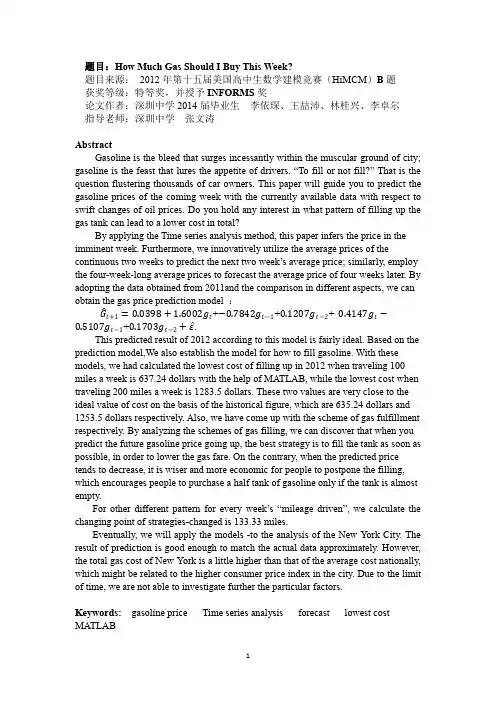
题目:How Much Gas Should I Buy This Week?题目来源:2012年第十五届美国高中生数学建模竞赛(HiMCM)B题获奖等级:特等奖,并授予INFORMS奖论文作者:深圳中学2014届毕业生李依琛、王喆沛、林桂兴、李卓尔指导老师:深圳中学张文涛AbstractGasoline is the bleed that surges incessantly within the muscular ground of city; gasoline is the feast that lures the appetite of drivers. “To fill or not fill?” That is the question flustering thousands of car owners. This paper will guide you to predict the gasoline prices of the coming week with the currently available data with respect to swift changes of oil prices. Do you hold any interest in what pattern of filling up the gas tank can lead to a lower cost in total?By applying the Time series analysis method, this paper infers the price in the imminent week. Furthermore, we innovatively utilize the average prices of the continuous two weeks to predict the next two week’s average price; similarly, employ the four-week-long average prices to forecast the average price of four weeks later. By adopting the data obtained from 2011and the comparison in different aspects, we can obtain the gas price prediction model :G t+1=0.0398+1.6002g t+−0.7842g t−1+0.1207g t−2+ 0.4147g t−0.5107g t−1+0.1703g t−2+ε .This predicted result of 2012 according to this model is fairly ideal. Based on the prediction model,We also establish the model for how to fill gasoline. With these models, we had calculated the lowest cost of filling up in 2012 when traveling 100 miles a week is 637.24 dollars with the help of MATLAB, while the lowest cost when traveling 200 miles a week is 1283.5 dollars. These two values are very close to the ideal value of cost on the basis of the historical figure, which are 635.24 dollars and 1253.5 dollars respectively. Also, we have come up with the scheme of gas fulfillment respectively. By analyzing the schemes of gas filling, we can discover that when you predict the future gasoline price going up, the best strategy is to fill the tank as soon as possible, in order to lower the gas fare. On the contrary, when the predicted price tends to decrease, it is wiser and more economic for people to postpone the filling, which encourages people to purchase a half tank of gasoline only if the tank is almost empty.For other different pattern for every week’s “mileage driven”, we calculate the changing point of strategies-changed is 133.33 miles.Eventually, we will apply the models -to the analysis of the New York City. The result of prediction is good enough to match the actual data approximately. However, the total gas cost of New York is a little higher than that of the average cost nationally, which might be related to the higher consumer price index in the city. Due to the limit of time, we are not able to investigate further the particular factors.Keywords: gasoline price Time series analysis forecast lowest cost MATLABAbstract ---------------------------------------------------------------------------------------1 Restatement --------------------------------------------------------------------------------------21. Assumption----------------------------------------------------------------------------------42. Definitions of Variables and Models-----------------------------------------------------4 2.1 Models for the prediction of gasoline price in the subsequent week------------4 2.2 The Model of oil price next two weeks and four weeks--------------------------5 2.3 Model for refuel decision-------------------------------------------------------------52.3.1 Decision Model for consumer who drives 100 miles per week-------------62.3.2 Decision Model for consumer who drives 200 miles per week-------------73. Train and Test Model by 2011 dataset---------------------------------------------------8 3.1 Determine the all the parameters in Equation ② from the 2011 dataset-------8 3.2 Test the Forecast Model of gasoline price by the dataset of gasoline price in2012-------------------------------------------------------------------------------------10 3.3 Calculating ε --------------------------------------------------------------------------12 3.4 Test Decision Models of buying gasoline by dataset of 2012-------------------143.4.1 100 miles per week---------------------------------------------------------------143.4.2 200 miles per week---------------------------------------------------------------143.4.3 Second Test for the Decision of buying gasoline-----------------------------154. The upper bound will change the Decision of buying gasoline---------------------155. An analysis of New York City-----------------------------------------------------------16 5.1 The main factor that will affect the gasoline price in New York City----------16 5.2 Test Models with New York data----------------------------------------------------185.3 The analysis of result------------------------------------------------------------------196. Summery& Advantage and disadvantage-----------------------------------------------197. Report----------------------------------------------------------------------------------------208. Appendix------------------------------------------------------------------------------------21 Appendix 1(main MATLAB programs) ------------------------------------------------21 Appendix 2(outcome and graph) --------------------------------------------------------34The world market is fluctuating swiftly now. As the most important limited energy, oil is much accounted of cars owners and dealer. We are required to make a gas-buying plan which relates to the price of gasoline, the volume of tank, the distance that consumer drives per week, the data from EIA and the influence of other events in order to help drivers to save money.We should use the data of 2011 to build up two models that discuss two situations: 100miles/week or 200miles/week and use the data of 2012 to test the models to prove the model is applicable. In the model, consumer only has three choices to purchase gas each week, including no gas, half a tank and full tank. At the end, we should not only build two models but also write a simple but educational report that can attract consumer to follow this model.1.Assumptiona)Assume the consumer always buy gasoline according to the rule of minimumcost.b)Ignore the difference of the gasoline weight.c)Ignore the oil wear on the way to gas stations.d)Assume the tank is empty at the beginning of the following models.e)Apply the past data of crude oil price to predict the future price ofgasoline.(The crude oil price can affect the gasoline price and we ignore thehysteresis effect on prices of crude oil towards prices of gasoline.)2.Definitions of Variables and Modelst stands for the sequence number of week in any time.(t stands for the current week. (t-1) stands for the last week. (t+1) stands for the next week.c t: Price of crude oil of the current week.g t: Price of gasoline of the t th week.P t: The volume of oil of the t th week.G t+1: Predicted price of gasoline of the (t+1)th week.α,β: The coefficient of the g t and c t in the model.d: The variable of decision of buying gasoline.(d=1/2 stands for buying a half tank gasoline)2.1 Model for the prediction of gasoline price in the subsequent weekWhether to buy half a tank oil or full tank oil depends on the short-term forecast about the gasoline prices. Time series analysis is a frequently-used method to expect the gasoline price trend. It can be expressed as:G t+1=α1g t+α2g t−1+α3g t−2+α4g t−3+…αn+1g t−n+ε ----Equation ①ε is a parameter that reflects the influence towards the trend of gasoline price in relation to several aspects such as weather data, economic data, world events and so on.Due to the prices of crude oil can influence the future prices of gasoline; we will adopt the past prices of crude oil into the model for gasoline price forecast.G t+1=(α1g t+α2g t−1+α3g t−2+α4g t−3+⋯αn+1g t−n)+(β1g t+β2g t−1+β3g t−2+β4g t−3+⋯βn+1g t−n)+ε----Equation ②We will use the 2011 data set to calculate the all coefficients and the best delay periods n.2.2 The Model of oil price next two weeks and four weeksWe mainly depend on the prediction of change of gasoline price in order to make decision that the consumer should buy half a tank or full tank gas. When consumer drives 100miles/week, he can drive whether 400miles most if he buys full tank gas or 200miles most if he buys half a tank gas. When consumer drives 200miles/week, full tank gas can be used two weeks most or half a tank can be used one week most. Thus, we should consider the gasoline price trend in four weeks in future.Equation ②can also be rewritten asG t+1=(α1g t+β1g t)+(α2g t−1+β2g t−1)+(α3g t−2+β3g t−2)+⋯+(αn+1g t−n+βn+1g t−n)+ε ----Equation ③If we define y t=α1g t+β1g t,y t−1=α2g t−1+β2g t−1, y t−2=α3g t−2+β3g t−2……, and so on.Equation ③can change toG t+1=y t+y t−1+y t−2+⋯+y t−n+ε ----Equation ④We use y(t−1,t)denote the average price from week (t-1) to week (t), which is.y(t−1,t)=y t−1+y t2Accordingly, the average price from week (t-3) to week (t) isy(t−3,t)=y t−3+y t−2+y t−1+y t.4Apply Time series analysis, we can get the average price from week (t+1) to week (t+2) by Equation ④,G(t+1,t+2)=y(t−1,t)+y(t−3,t−2)+y(t−5,t−4), ----Equation ⑤As well, the average price from week (t+1) to week (t+4) isG(t+1,t+4)=y(t−3,t)+y(t−7,t−4)+y(t−11,t−8). ----Equation ⑥2.3 Model for refuel decisionBy comparing the present gasoline price with the future price, we can decide whether to fill half or full tank.The process for decision can be shown through the following flow chart.Chart 1For the consumer, the best decision is to get gasoline with the lowest prices. Because a tank of gasoline can run 2 or 4 week, so we should choose a time point that the price is lowest by comparison of the gas prices at present, 2 weeks and 4 weeks later separately. The refuel decision also depends on how many free spaces in the tank because we can only choose half or full tank each time. If the free spaces are less than 1/2, we can refuel nothing even if we think the price is the lowest at that time.2.3.1 Decision Model for consumer who drives 100 miles per week.We assume the oil tank is empty at the beginning time(t=0). There are four cases for a consumer to choose a best refuel time when the tank is empty.i.g t>G t+4and g t>G t+2, which means the present gasoline price is higherthan that either two weeks or four weeks later. It is economic to fill halftank under such condition. ii. g t <Gt +4 and g t <G t +2, which means the present gasoline price is lower than that either two weeks or four weeks later. It is economic to fill fulltank under such condition. iii. Gt +4>g t >G t +2, which means the present gasoline price is higher than that two weeks later but lower than that four weeks later. It is economic to fillhalf tank under such condition. iv. Gt +4<g t <G t +2, which means the present gasoline price is higher than that four weeks later but lower than that two weeks later. It is economic to fillfull tank under such condition.If other time, we should consider both the gasoline price and the oil volume in the tank to pick up a best refuel time. In summary, the decision model for running 100 miles a week ist 2t 4t 2t 4t 2t 4t 2t 4t 11111411111ˆˆ(1)1((1)&max(,))24442011111ˆˆˆˆ1/2((1)&G G G (&))(0(1G G )&)4424411ˆˆˆ(1)0&(G 4G G (G &)t i t i t t t t i t i t t t t t t i t t d t or d t g d d t g or d t g d t g or ++++----+++-++<--<<--<>⎧⎪=<--<<<--<<<⎨⎪⎩--=><∑∑∑∑∑t 2G ˆ)t g +<----Equation ⑦d i is the decision variable, d i =1 means we fill full tank, d i =1/2 means we fill half tank. 11(1)4t i tdt ---∑represents the residual gasoline volume in the tank. The method of prices comparison was analyzed in the beginning part of 2.3.1.2.3.2 Decision Model for consumer who drives 200 miles per week.Because even full tank can run only two weeks, the consumer must refuel during every two weeks. There are two cases to decide whether to buy half or full tank when the tank is empty. This situation is much simpler than that of 100 miles a week. The process for decision can also be shown through the following flow chart.Chart 2The two cases for deciding buy half or full tank are: i. g t >Gt +1, which means the present gasoline price is higher than the next week. We will buy half tank because we can buy the cheaper gasoline inthe next week. ii. g t <Gt +1, which means the present gasoline price is lower than the next week. To buy full tank is economic under such situation.But we should consider both gasoline prices and free tank volume to decide our refueling plan. The Model is111t 11t 111(1)1220111ˆ1/20(1)((1)0&)22411ˆ(1&G )0G 2t i t t i t i t t t t t i t t d t d d t or d t g d t g ----++<--<⎧⎪=<--<--=>⎨⎪⎩--=<∑∑∑∑ ----Equation ⑧3. Train and Test Model by the 2011 datasetChart 33.1 Determine all the parameters in Equation ② from the 2011 dataset.Using the weekly gas data from the website and the weekly crude price data from , we can determine the best delay periods n and calculate all the parameters in Equation ②. For there are two crude oil price dataset (Weekly Cushing OK WTI Spot Price FOB and Weekly Europe Brent SpotPrice FOB), we use the average value as the crude oil price without loss of generality. We tried n =3, 4 and 5 respectively with 2011 dataset and received comparison graph of predicted value and actual value, including corresponding coefficient.(A ) n =3(the hysteretic period is 3)Graph 1 The fitted price and real price of gasoline in 2011(n=3)We find that the nearby effect coefficient of the price of crude oil and gasoline. This result is same as our anticipation.(B)n=4(the hysteretic period is 4)Graph 2 The fitted price and real price of gasoline in 2011(n=4)(C) n=5(the hysteretic period is 5)Graph 3 The fitted price and real price of gasoline in 2011(n=5)Via comparing the three figures above, we can easily found that the predictive validity of n=3(the hysteretic period is 3) is slightly better than that of n=4(the hysteretic period is 4) and n=5(the hysteretic period is 5) so we choose the model of n=3 to be the prediction model of gasoline price.G t+1=0.0398+1.6002g t+−0.7842g t−1+0.1207g t−2+ 0.4147g t−0.5107g t−1+0.1703g t−2+ε----Equation ⑨3.2 Test the Forecast Model of gasoline price by the dataset of gasoline price in 2012Next, we apply models in terms of different hysteretic periods(n=3,4,5 respectively), which are shown in Equation ②,to forecast the gasoline price which can be acquired currently in 2012 and get the graph of the forecast price and real price of gasoline:Graph 4 The real price and forecast price in 2012(n=3)Graph 5 The real price and forecast price in 2012(n=4)Graph 6 The real price and forecast price in 2012(n=5)Conserving the error of observation, predictive validity is best when n is 3, but the differences are not obvious when n=4 and n=5. However, a serious problem should be drawn to concerns: consumers determines how to fill the tank by using the trend of oil price. If the trend prediction is wrong (like predicting oil price will rise when it actually falls), consumers will lose. We use MATLAB software to calculate the amount of error time when we use the model of Equation ⑨to predict the price of gasoline in 2012. The graph below shows the result.It’s not difficult to find the prediction effect is the best when n is 3. Therefore, we determined to use Equation ⑨as the prediction model of oil price in 2012.G t+1=0.0398+1.6002g t+−0.7842g t−1+0.1207g t−2+ 0.4147g t−0.5107g t−1+0.1703g t−2+ε3.3 Calculating εSince political occurences, economic events and climatic changes can affect gasoline price, it is undeniable that a ε exists between predicted prices and real prices. We can use Equation ②to predict gasoline prices in 2011 and then compare them with real data. Through the difference between predicted data and real data, we can estimate the value of ε .The estimating process can be shown through the following flow chartChart 4We divide the international events into three types: extra serious event, major event and ordinary event according to the criteria of influence on gas prices. Then we evaluate the value: extra serious event is 3a, major event is 2a, and ordinary event is a. With inference to the comparison of the forecast price and real price in 2011, we find that large deviation of data exists at three time points: May 16,2011, Aug 08,2011 andOct 10,2011. After searching, we find that some important international events happened nearly at the three time points. We believe that these events which occurred by chance affect the international prices of gasoline so the predicted prices deviate from the actual prices. The table of events and the calculation of the value of a areTherefore, by generalizing several sets of particular data and events, we can estimate the value of a:a=26.84 ----Equation ⑩The calculating process is shown as the following graph.Since now we have obtained the approximate value of a, we can evaluate the future prices according to currently known gasoline prices and crude oil prices. To improve our model, we can look for factors resulting in some major turning point in the graph of gasoline prices. On the ground that the most influential factors on prices in 2012 are respectively graded, the difference between fact and prediction can be calculated.3.4 Test Decision Models of buying gasoline by the dataset of 2012First, we use Equation ⑨to calculate the gasoline price of next week and use Equation ⑤and Equation ⑥to calculate the gasoline price trend of next two to four weeks. On the basis above, we calculate the total cost, and thus receive schemes of buying gasoline of 100miles per week according to Equation ⑦and Equation ⑧. Using the same method, we can easily obtain the pattern when driving 200 miles per week. The result is presented below.We collect the important events which will affect the gasoline price in 2012 as well. Therefore, we calculate and adjust the predicted price of gasoline by Equation ⑩. We calculate the scheme of buying gasoline again. The result is below:3.4.1 100 miles per weekT2012 = 637.2400 (If the consumer drives 100 miles per week, the total cost inTable 53.4.2 200 miles per weekT2012 = 1283.5 (If the consumer drives 200 miles per week, the total cost in 2012 is 1283.5 USD). The scheme calculated by software is below:Table 6According to the result of calculating the buying-gasoline scheme from the model, we can know: when the gasoline price goes up, we should fill up the tank first and fill up again immediately after using half of gasoline. It is economical to always keep the tank full and also to fill the tank in advance in order to spend least on gasoline fee. However, when gasoline price goes down, we have to use up gasoline first and then fill up the tank. In another words, we need to delay the time of filling the tank in order to pay for the lowest price. In retrospect to our model, it is very easy to discover that the situation is consistent with life experience. However, there is a difference. The result is based on the calculation from the model, while experience is just a kind of intuition.3.4.3 Second Test for the Decision of buying gasolineSince the data in 2012 is historical data now, we use artificial calculation to get the optimal value of buying gasoline. The minimum fee of driving 100 miles per week is 635.7440 USD. The result of calculating the model is 637.44 USD. The minimum fee of driving 200 miles per week is 1253.5 USD. The result of calculating the model is 1283.5 USD. The values we calculate is close to the result of the model we build. It means our model prediction effect is good. (we mention the decision people made every week and the gas price in the future is unknown. We can only predict. It’s normal to have deviation. The buying-gasoline fee which is based on predicted calculation must be higher than the minimum buying-gasoline fee which is calculated when all the gas price data are known.)We use MATLAB again to calculate the total buying-gasoline fee when n=4 and n=5. When n=4,the total fee of driving 100 miles per week is 639.4560 USD and the total fee of driving 200 miles per week is 1285 USD. When n=5, the total fee of driving 100 miles per week is 639.5840 USD and the total fee of driving 200 miles per week is 1285.9 USD. The total fee are all higher the fee when n=3. It means it is best for us to take the average prediction model of 3 phases.4. The upper bound will change the Decision of buying gasoline.Assume the consumer has a mileage driven of x1miles per week. Then, we can use 200to indicate the period of consumption, for half of a tank can supply 200-mile x1driving. Here are two situations:<1.5①200x1>1.5②200x1In situation①, the consumer is more likely to apply the decision of 200-mile consumer’s; otherwise, it is wiser to adopt the decision of 100-mile consumer’s. Therefore, x1is a critical value that changes the decision if200=1.5x1x1=133.3.Thus, the mileage driven of 133.3 miles per week changes the buying decision.Then, we consider the full-tank buyers likewise. The 100-mile consumer buys half a tank once in four weeks; the 200-mile consumer buys half a tank once in two weeks. The midpoint of buying period is 3 weeks.Assume the consumer has a mileage driven of x2miles per week. Then, we can to illustrate the buying period, since a full tank contains 400 gallons. There use 400x2are still two situations:<3③400x2>3④400x2In situation③, the consumer needs the decision of 200-mile consumer’s to prevent the gasoline from running out; in the latter situation, it is wiser to tend to the decision of 100-mile consumer’s. Therefore, x2is a critical value that changes the decision if400=3x2x2=133.3We can find that x2=x1=133.3.To wrap up, there exists an upper bound on “mileage driven”, that 133.3 miles per week is the value to switch the decision for buying weekly gasoline. The following picture simplifies the process.Chart 45. An analysis of New Y ork City5.1 The main factors that will affect the gasoline price in New York CityBased on the models above, we decide to estimate the price of gasoline according to the data collected and real circumstances in several cities. Specifically, we choose New York City as a representative one.New York City stands in the North East in the United States, with the largest population throughout the country as 8.2 million. The total area of New York City is around 1300 km2, with the land area as 785.6 km2(303.3 mi2). One of the largest trading centers in the world, New York City has a high level of resident’s consumption. As a result, the level of the price of gasoline in New York City is higher than the average regular oil price of the United States. The price level of gasoline and its fluctuation are the main factors of buying decision.Another reasonable factor we expect is the distribution of gas stations. According to the latest report, there are approximately 1670 gas stations in the city area (However, after the impact of hurricane Sandy, about 90 gas stations have been temporarily out of use because of the devastation of Sandy, and there is still around 1580 stations remaining). From the information above, we can calculate the density of gas stations thatD(gasoline station)= t e amount of gas stationstotal land area =1670 stations303.3 mi2=5.506 stations per mi2This is a respectively high value compared with several other cities the United States. It also indicates that the average distance between gas stations is relatively small. The fact that we can neglect the distance for the cars to get to the station highlights the role of the fluctuation of the price of gasoline in New York City.Also, there are approximately 1.8 million residents of New York City hold the driving license. Because the exact amount of cars in New York City is hard to determine, we choose to analyze the distribution of possible consumers. Thus, we can directly estimate the density of consumers in New York City in a similar way as that of gas stations:D(gasoline consumers)= t e amount of consumerstotal land area = 1.8 million consumers303.3 mi2=5817consumers per mi2Chart 5In addition, we expect that the fluctuation of the price of crude oil plays a critical role of the buying decision. The media in New York City is well developed, so it is convenient for citizens to look for the data of the instant price of crude oil, then to estimate the price of gasoline for the coming week if the result of our model conforms to the assumption. We will include all of these considerations in our modification of the model, which we will discuss in the next few steps.For the analysis of New York City, we apply two different models to estimate the price and help consumers make the decision.5.2 Test Models with New York dataAmong the cities in US, we pick up New York as an typical example. The gas price data is downloaded from the website () and is used in the model described in Section 2 and 3.The gas price curves between the observed data and prediction data are compared in next Figure.Figure 6The gas price between the observed data and predicted data of New York is very similar to Figure 3 in US case.Since there is little difference between the National case and New York case, the purchase strategy is same. Following the same procedure, we can compare the gas cost between the historical result and predicted result.For the case of 100 miles per week, the total cost of observed data from Feb to Oct of 2012 in New York is 636.26USD, while the total cost of predicted data in the same period is 638.78USD, which is very close. It proves that our prediction model is good. For the case of 200 miles per week, the total cost of observed data from Feb to Oct of 2012 in New York is 1271.2USD, while the total cost of predicted data in the same period is 1277.6USD, which is very close. It proves that our prediction model is good also.5.3 The analysis of resultBy comparing, though density of gas stations and density of consumers of New York is a little higher than other places but it can’t lower the total buying-gas fee. Inanother words, density of gas stations and density of consumers are not the actual factors of affecting buying-gas fee.On the other hand, we find the gas fee in New York is a bit higher than the average fee in US. We can only analyze preliminary it is because of the higher goods price in New York. We need to add price factor into prediction model. We can’t improve deeper because of the limited time. The average CPI table of New York City and USA is below:Datas Statistics website(/xg_shells/ro2xg01.htm)6. Summery& Advantage and disadvantageTo reach the solution, we make graphs of crude oil and gasoline respectively and find the similarity between them. Since the conditions are limited that consumers can only drive 100miles per week or 200miles per week, we separate the problem into two parts according to the limitation. we use Time series analysis Method to predict the gasoline price of a future period by the data of several periods in the past. Then we take the influence of international events, economic events and weather changes and so on into consideration by adding a parameter. We give each factor a weight consequently and find the rules of the solution of 100miles per week and 200miles per week. Then we discuss the upper bound and clarify the definition of upper bound to solve the problem.According to comparison from many different aspects, we confirm that the model expressed byEquation ⑨is the best. On the basis of historical data and the decision model of buying gasoline(Equation ⑦and Equation ⑧), we calculate that the actual least cost of buying gasoline is 635.7440 USD if the consumer drives 100 miles per week (the result of our model is 637.24 USD) and the actual least cost of buying gasoline is 1253.5 USD(the result of our model is 1283.5 USD) if the consumer drives 100 miles per week. The result we predicted is similar to the actual result so the predictive validity of our model is finer.Disadvantages:1.The events which we predicted are difficult to quantize accurately. The turningpoint is difficult for us to predict accurately as well.2.We only choose two kinds of train of thought to develop models so we cannotevaluate other methods that we did not discuss in this paper. Other models which are built up by other train of thought are possible to be the optimal solution.。
美国数学建模竞赛优秀论文阅读报告
2.优秀论文一具体要求:1月28日上午汇报1)论文主要内容、具体模型和求解算法(针对摘要和全文进行概括);In the part1, we will design a schedule with fixed trip dates and types and also routes. In the part2, we design a schedule with fixed trip dates and types but unrestrained routes.In the part3, we design a schedule with fixed trip dates but unrestrained types and routes.In part 1, passengers have to travel along the rigid route set by river agency, so the problem should be to come up with the schedule to arrange for the maximum number of trips without occurrence of two different trips occupying the same campsite on the same day.In part 2, passengers have the freedom to choose which campsites to stop at, therefore the mathematical description of their actions inevitably involve randomness and probability, and we actually use a probability model. The next campsite passengers choose at a current given campsite is subject to a certain distribution, and we describe events of two trips occupying the same campsite y probability. Note in probability model it is no longer appropriate to say that two trips do not meet at a campsite with certainty; instead, we regard events as impossible if their probabilities are below an adequately small number. Then we try to find the optimal schedule.In part 3, passengers have the freedom to choose both the type and route of the trip; therefore a probability model is also necessary. We continue to adopt the probability description as in part 2 and then try to find the optimal schedule.In part 1, we find the schedule of trips with fixed dates, types (propulsion and duration) and routes (which campsites the trip stops at), and to achieve this we use a rather novel method. The key idea is to divide campsites into different “orbits”that only allows some certain trip types to travel in, therefore the problem turns into several separate small problem to allocate fewer trip types, and the discussion of orbits allowing one, two, three trip types lead to general result which can deal with any value of Y. Particularly, we let Y=150, a rather realistic number of campsites, to demonstrate a concrete schedule and the carrying capacity of the river is 2340 trips.In part 2, we find the schedule of trips with fixed dates, types but unrestrained routes. To better describe the behavior of tourists, we need to use a stochastic model(随机模型). We assume a classical probability model and also use the upper limit value of small probability to define an event as not happening. Then we use Greedy algorithm to choose the trips added and recursive algorithm together with Jordan Formula to calculate the probability of two trips simultaneously occupying the same campsites. The carrying capacity of the river by this method is 500 trips. This method can easily find theoptimal schedule with X given trips, no matter these X trips are with fixed routes or not. In part 3, we find the optimal schedule of trips with fixed dates and unrestrained types and routes. This is based on the probability model developed in part 2 and we assign the choice of trip types of the tourists with a uniform distribution to describe their freedom to choose and obtain the results similar to part 2. The carrying capacity of the river by this method is 493 trips. Also this method can easily find the optimal schedule with X given trips, no matter these X trips are with fixed routes or not.2)论文结构概述(列出提纲,分析优缺点,自己安排的结构);1 Introduction2 Definitions3 Specific formulation of problem4 Assumptions5 Part 1 Best schedule of trips with fixed dates, types and also routes.5.1 Method5.1.1 Motivation and justification5.1.2 Key ideas5.2 Development of the model5.2.1Every campsite set for every single trip type5.2.2 Every campsite set for every multiple trip types5.2.3One campsite set for all trip types6 Part 2 Best schedule of trips with fixed dates and types, but unrestrained routes.6.1 Method6.1.1 Motivation and justification6.1.2 Key ideas6.2 Development of the model6.2.1 Calculation of p(T,x,t)6.2.2 Best schedule using Greedy algorithm6.2.3 Application to situation where X trips are given7 Part 3 Best schedule of trips with fixed dates, but unrestrained types and routes.7.1 Method7.1.1 Motivation and justification7.1.2 Key ideas7.2 Development of the model8 Testing of the model----Sensitivity analysis8.1Stability with varying trip types chosen in 68.2The sensitivity analysis of the assumption 4④8.3 The sensitivity analysis of the assumption 4⑥9 Evaluation of the model9.1 Strengths and weaknesses9.1.1 Strengths9.1.2 Weakness9.2 Further discussion10 Conclusions11 References12 Letter to the river managers3)论文中出现的好词好句(做好记录);用于问题的转化We regard the carrying capacity of the river as the maximum total number of trips available each year, hence turning the task of the river managers into looking for the best schedule itself.表明我们在文中所做的工作We have examined many policies for different river…..问题的分解We mainly divide the problem into three parts and come up with three different….对我们工作的要求:Given the above considerations, we want to find the optimal。
数学建模美赛一等奖优秀专业论文
For office use onlyT1________________ T2________________ T3________________ T4________________ Team Control Number52888Problem ChosenAFor office use onlyF1________________F2________________F3________________F4________________Mathematical Contest in Modeling (MCM/ICM) Summary SheetSummaryIt’s pleasant t o go home to take a bath with the evenly maintained temperature of hot water throughout the bathtub. This beautiful idea, however, can not be always realized by the constantly falling water temperature. Therefore, people should continually add hot water to keep the temperature even and as close as possible to the initial temperature without wasting too much water. This paper proposes a partial differential equation of the heat conduction of the bath water temperature, and an object programming model. Based on the Analytic Hierarchy Process (AHP) and Technique for Order Preference by Similarity to Ideal Solution (TOPSIS), this paper illustrates the best strategy the person in the bathtub can adopt to satisfy his desires. First, a spatiotemporal partial differential equation model of the heat conduction of the temperature of the bath water is built. According to the priority, an object programming model is established, which takes the deviation of temperature throughout the bathtub, the deviation of temperature with the initial condition, water consumption, and the times of switching faucet as the four objectives. To ensure the top priority objective—homogenization of temperature, the discretization method of the Partial Differential Equation model (PDE) and the analytical analysis are conducted. The simulation and analytical results all imply that the top priority strategy is: The proper motions of the person making the temperature well-distributed throughout the bathtub. Therefore, the Partial Differential Equation model (PDE) can be simplified to the ordinary differential equation model.Second, the weights for the remaining three objectives are determined based on the tolerance of temperature and the hobby of the person by applying Analytic Hierarchy Process (AHP) and Technique for Order Preference by Similarity to Ideal Solution (TOPSIS). Therefore, the evaluation model of the synthesis score of the strategy is proposed to determine the best one the person in the bathtub can adopt. For example, keeping the temperature as close as the initial condition results in the fewer number of switching faucet while attention to water consumption gives rise to the more number. Third, the paper conducts the analysis of the diverse parameters in the model to determine the best strategy, respectively, by controlling the other parameters constantly, and adjusting the parameters of the volume, shape of the bathtub and the shape, volume, temperature and the motions and other parameters of the person in turns. All results indicate that the differential model and the evaluation model developed in this paper depends upon the parameters therein. When considering the usage of a bubble bath additive, it is equal to be the obstruction between water and air. Our results show that this strategy can reduce the dropping rate of the temperatureeffectively, and require fewer number of switching.The surface area and heat transfer coefficient can be increased because of the motions of the person in the bathtub. Therefore, the deterministic model can be improved as a stochastic one. With the above evaluation model, this paper present the stochastic optimization model to determine the best strategy. Taking the disparity from the initial temperature as the suboptimum objectives, the result of the model reveals that it is very difficult to keep the temperature constant even wasting plentiful hot water in reality.Finally, the paper performs sensitivity analysis of parameters. The result shows that the shape and the volume of the tub, different hobbies of people will influence the strategies significantly. Meanwhile, combine with the conclusion of the paper, we provide a one-page non-technical explanation for users of the bathtub.Fall in love with your bathtubAbstractIt’s pleasant t o go home to take a bath with the evenly maintained temperature of hot water throughout the bathtub. This beautiful idea, however, can not be always realized by the constantly falling water temperature. Therefore, people should continually add hot water to keep the temperature even and as close as possible to the initial temperature without wasting too much water. This paper proposes a partial differential equation of the heat conduction of the bath water temperature, and an object programming model. Based on the Analytic Hierarchy Process (AHP) and Technique for Order Preference by Similarity to Ideal Solution (TOPSIS), this paper illustrates the best strategy the person in the bathtub can adopt to satisfy his desires. First, a spatiotemporal partial differential equation model of the heat conduction of the temperature of the bath water is built. According to the priority, an object programming model is established, which takes the deviation of temperature throughout the bathtub, the deviation of temperature with the initial condition, water consumption, and the times of switching faucet as the four objectives. To ensure the top priority objective—homogenization of temperature, the discretization method of the Partial Differential Equation model (PDE) and the analytical analysis are conducted. The simulation and analytical results all imply that the top priority strategy is: The proper motions of the person making the temperature well-distributed throughout the bathtub. Therefore, the Partial Differential Equation model (PDE) can be simplified to the ordinary differential equation model.Second, the weights for the remaining three objectives are determined based on the tolerance of temperature and the hobby of the person by applying Analytic Hierarchy Process (AHP) and Technique for Order Preference by Similarity to Ideal Solution (TOPSIS). Therefore, the evaluation model of the synthesis score of the strategy is proposed to determine the best one the person in the bathtub can adopt. For example, keeping the temperature as close as the initial condition results in the fewer number of switching faucet while attention to water consumption gives rise to the more number. Third, the paper conducts the analysis of the diverse parameters in the model to determine the best strategy, respectively, by controlling the other parameters constantly, and adjusting the parameters of the volume, shape of the bathtub and the shape, volume, temperature and the motions and other parameters of the person in turns. All results indicate that the differential model and the evaluation model developed in this paper depends upon the parameters therein. When considering the usage of a bubble bath additive, it is equal to be the obstruction between water and air. Our results show that this strategy can reduce the dropping rate of the temperature effectively, and require fewer number of switching.The surface area and heat transfer coefficient can be increased because of the motions of the person in the bathtub. Therefore, the deterministic model can be improved as a stochastic one. With the above evaluation model, this paper present the stochastic optimization model to determine the best strategy. Taking the disparity from the initial temperature as the suboptimum objectives, the result of the model reveals that it is very difficult to keep the temperature constant even wasting plentiful hotwater in reality.Finally, the paper performs sensitivity analysis of parameters. The result shows that the shape and the volume of the tub, different hobbies of people will influence the strategies significantly. Meanwhile, combine with the conclusion of the paper, we provide a one-page non-technical explanation for users of the bathtub.Keywords:Heat conduction equation; Partial Differential Equation model (PDE Model); Objective programming; Strategy; Analytical Hierarchy Process (AHP) Problem StatementA person fills a bathtub with hot water and settles into the bathtub to clean and relax. However, the bathtub is not a spa-style tub with a secondary hearing system, as time goes by, the temperature of water will drop. In that conditions,we need to solve several problems:(1) Develop a spatiotemporal model of the temperature of the bathtub water to determine the best strategy to keep the temperature even throughout the bathtub and as close as possible to the initial temperature without wasting too much water;(2) Determine the extent to which your strategy depends on the shape and volume of the tub, the shape/volume/temperature of the person in the bathtub, and the motions made by the person in the bathtub.(3)The influence of using b ubble to model’s results.(4)Give a one-page non-technical explanation for users that describes your strategyGeneral Assumptions1.Considering the safety factors as far as possible to save water, the upper temperature limit is set to 45 ℃;2.Considering the pleasant of taking a bath, the lower temperature limit is set to 33℃;3.The initial temperature of the bathtub is 40℃.Table 1Model Inputs and SymbolsSymbols Definition UnitT Initial temperature of the Bath water ℃℃T∞Outer circumstance temperatureT Water temperature of the bathtub at the every moment ℃t Time hx X coordinates of an arbitrary point my Y coordinates of an arbitrary point mz Z coordinates of an arbitrary point mαTotal heat transfer coefficient of the system 2()⋅/W m K1SThe surrounding-surface area of the bathtub 2m 2S The above-surface area of water2m 1H Bathtub’s thermal conductivity/W m K ⋅() D The thickness of the bathtub wallm 2H Convection coefficient of water2/W m K ⋅() a Length of the bathtubm b Width of the bathtubm h Height of the bathtubm V The volume of the bathtub water3m c Specific heat capacity of water/()J kg ⋅℃ ρ Density of water3/kg m ()v t Flooding rate of hot water3/m s r TThe temperature of hot water ℃Temperature ModelBasic ModelA spatio-temporal temperature model of the bathtub water is proposed in this paper. It is a four dimensional partial differential equation with the generation and loss of heat. Therefore the model can be described as the Thermal Equation.The three-dimension coordinate system is established on a corner of the bottom of the bathtub as the original point. The length of the tub is set as the positive direction along the x axis, the width is set as the positive direction along the y axis, while the height is set as the positive direction along the z axis, as shown in figure 1.Figure 1. The three-dimension coordinate systemTemperature variation of each point in space includes three aspects: one is the natural heat dissipation of each point in space; the second is the addition of exogenous thermal energy; and the third is the loss of thermal energy . In this way , we build the Partial Differential Equation model as follows:22212222(,,,)(,,,)()f x y z t f x y z t T T T T t x y z c Vαρ-∂∂∂∂=+++∂∂∂∂ (1) Where● t refers to time;● T is the temperature of any point in the space;● 1f is the addition of exogenous thermal energy;● 2f is the loss of thermal energy.According to the requirements of the subject, as well as the preferences of people, the article proposes these following optimization objective functions. A precedence level exists among these objectives, while keeping the temperature even throughout the bathtub must be ensured.Objective 1(.1O ): keep the temperature even throughout the bathtub;22100min (,,,)(,,,)t t V V F t T x y z t dxdydz dt t T x y z t dxdydz dt ⎡⎤⎡⎤⎛⎫=-⎢⎥ ⎪⎢⎥⎢⎥⎣⎦⎝⎭⎣⎦⎰⎰⎰⎰⎰⎰⎰⎰ (2) Objective 2(.2O ): keep the temperature as close as possible to the initial temperature;[]2200min (,,,)tV F T x y z t T dxdydz dt ⎛⎫=- ⎪⎝⎭⎰⎰⎰⎰ (3) Objective 3(.3O ): do not waste too much water;()30min tF v t dt =⋅⎰ (4) Objective 4(.4O ): fewer times of switching.4min F n = (5)Since the .1O is the most crucial, we should give priority to this objective. Therefore, the highest priority strategy is given here, which is homogenization of temperature.Strategy 0 – Homogenization of T emperatureThe following three reasons are provided to prove the importance of this strategy. Reason 1-SimulationIn this case, we use grid algorithm to make discretization of the formula (1), and simulate the distribution of water temperature.(1) Without manual intervention, the distribution of water temperature as shown infigure 2. And the variance of the temperature is 0.4962. 00.20.40.60.8100.51 1.5200.5Length WidthH e i g h t 4242.54343.54444.54545.5Distribution of temperature at the length=1Distribution of temperatureat the width=1Hot water Cool waterFigure 2. Temperature profiles in three-dimension space without manual intervention(2) Adding manual intervention, the distribution of water temperature as shown infigure 3. And the variance of the temperature is 0.005. 00.5100.51 1.5200.5 Length WidthH e i g h t 44.744.7544.844.8544.944.9545Distribution of temperatureat the length=1Distribution of temperature at the width=1Hot water Cool waterFigure 3. Temperature profiles in three-dimension space with manual interventionComparing figure 2 with figure 3, it is significant that the temperature of water will be homogeneous if we add some manual intervention. Therefore, we can assumed that222222()0T T T x y zα∂∂∂++≠∂∂∂ in formula (1). Reason 2-EstimationIf the temperature of any point in the space is different, then222222()0T T T x y zα∂∂∂++≠∂∂∂ Thus, we find two points 1111(,,,)x y z t and 2222(,,,)x y z t with:11112222(,,,)(,,,)T x y z t T x y z t ≠Therefore, the objective function 1F could be estimated as follows:[]2200200001111(,,,)(,,,)(,,,)(,,,)0t t V V t T x y z t dxdydz dt t T x y z t dxdydz dt T x y z t T x y z t ⎡⎤⎡⎤⎛⎫-⎢⎥ ⎪⎢⎥⎢⎥⎣⎦⎝⎭⎣⎦≥->⎰⎰⎰⎰⎰⎰⎰⎰ (6) The formula (6) implies that some motion should be taken to make sure that the temperature can be homogeneous quickly in general and 10F =. So we can assumed that: 222222()0T T T x y zα∂∂∂++≠∂∂∂. Reason 3-Analytical analysisIt is supposed that the temperature varies only on x axis but not on the y-z plane. Then a simplified model is proposed as follows:()()()()()()()2sin 000,0,,00,000t xx x T a T A x l t l T t T l t t T x x l π⎧=+≤≤≤⎪⎪⎪==≤⎨⎪⎪=≤≤⎪⎩ (7)Then we use two ways, Fourier transformation and Laplace transformation, in solving one-dimensional heat equation [Qiming Jin 2012]. Accordingly, we get the solution:()()2222/22,1sin a t l Al x T x t e a l πππ-=- (8) Where ()0,2x ∈, 0t >, ()01|x T f t ==(assumed as a constant), 00|t T T ==.Without general assumptions, we choose three specific value of t , and gain a picture containing distribution change of temperature in one-dimension space at different time.00.20.40.60.811.2 1.4 1.6 1.8200.511.522.533.54Length T e m p e r a t u r e time=3time=5time=8Figure 4. Distribution change of temperature in one-dimension space at different timeT able 2.V ariance of temperature at different timet3 5 8 variance0.4640 0.8821 1.3541It is noticeable in Figure 4 that temperature varies sharply in one-dimensional space. Furthermore, it seems that temperature will vary more sharply in three-dimension space. Thus it is so difficult to keep temperature throughout the bathtub that we have to take some strategies.Based on the above discussion, we simplify the four dimensional partial differential equation to an ordinary differential equation. Thus, we take the first strategy that make some motion to meet the requirement of homogenization of temperature, that is 10F =.ResultsTherefore, in order to meet the objective function, water temperature at any point in the bathtub needs to be same as far as possible. We can resort to some strategies to make the temperature of bathtub water homogenized, which is (,,)x y z ∀∈∀. That is,()(),,,T x y z t T t =Given these conditions, we improve the basic model as temperature does not change with space.112213312()()()()/()p r H S dT H S T T H S T T c v T T c V V dt D μρρ∞⎡⎤=++-+-+--⎢⎥⎣⎦(9) Where● 1μis the intensity of people’s movement ;● 3H is convection between water and people;● 3S is contact area between water and people;● p T is body surface temperature;● 1V is the volume of the bathtub;● 2V is the volume of people.Where the μ refers to the intensity of people ’s movement. It is a constant. However , it is a random variable in reality, which will be taken into consideration in the following.Model T estingWe use the oval-shaped bathtub to test our model. According to the actual situation, we give initial values as follows:0.19λ=,0.03D =,20.54H =,25T ∞=,040T =00.20.40.60.8125303540Time T e m p e r a t u r eFigure 5. Basic modelThe Figure 5 shows that the temperature decreases monotonously with time. And some signs of a slowing down in the rate of decrease are evident in the picture. Reaching about two hours, the water temperature does not change basically and be closely to the room temperature. Obviously , it is in line with the actual situation, indicating the rationality of this model.ConclusionOur model is robust under reasonable conditions, as can be seen from the testing above. In order to keep the temperature even throughout the bathtub, we should take some strategies like stirring constantly while adding hot water to the tub. Most important of all, this is the necessary premise of the following question.Strategy 1 – Fully adapted to the hot water in the tubInfluence of body surface temperatureWe select a set of parameters to simulate two kinds of situation separately.The first situation is that do not involve the factor of human1122()()/H S dT H S T T cV dt D ρ∞⎡⎤=+-⎢⎥⎣⎦(10) The second situation is that involves the factor of human112213312()()()/()p H S dT H S T T H S T T c V V dt D μρ∞⎡⎤=++-+--⎢⎥⎣⎦(11) According to the actual situation, we give specific values as follows, and draw agraph of temperature of two functions.33p T =,040T =204060801001201401601803838.53939.540TimeT e m p e r a t u r eWith body Without bodyFigure 6a. Influence of body surface temperature50010001500200025003000350025303540TimeT e m p e r a t u r eWith body Without bodyCoincident pointFigure 6b. Influence of body surface temperatureThe figure 6 shows the difference between two kinds of situation in the early time (before the coincident point ), while the figure 7 implies that the influence of body surface temperature reduces as time goes by . Combing with the degree of comfort ofbath and the factor of health, we propose the second optimization strategy: Fully adapted to the hot water after getting into the bathtub.Strategy 2 –Adding water intermittentlyInfluence of adding methods of waterThere are two kinds of adding methods of water. One is the continuous; the other is the intermittent. We can use both different methods to add hot water.1122112()()()/()r H S dT H S T T c v T T c V V dt D μρρ∞⎡⎤=++-+--⎢⎥⎣⎦(12) Where r T is the temperature of the hot water.To meet .3O , we calculated the minimum water consumption by changing the flow rate of hot water. And we compared the minimum water consumptions of the continuous with the intermittent to determine which method is better.A . Adding water continuouslyAccording to the actual situation, we give specific values as follows and draw a picture of the change of temperature.040T =, 37d T =, 45r T =5001000150020002500300035003737.53838.53939.54040.5TimeT e m p e r a t u r eadd hot waterFigure 7. Adding water continuouslyIn most cases, people are used to have a bath in an hour. Thus we consumed that deadline of the bath: 3600final t =. Then we can find the best strategy in Figure 5 which is listed in Table 2.T able 3Strategy of adding water continuouslystart t final tt ∆ vr T varianceWater flow 4 min 1 hour56 min537.410m s -⨯45℃31.8410⨯0.2455 3mB . Adding water intermittentlyMaintain the values of 0T ,d T ,r T ,v , we change the form of adding water, and get another graph.5001000150020002500300035003737.53838.53939.540TimeT e m p e r a t u r et1=283(turn on)t3=2107(turn on)t2=1828(turn off)Figure 8. Adding water intermittentlyT able 4.Strategy of adding water intermittently()1t on ()2t off 3()t on vr T varianceWater flow 5 min 30 min35min537.410m s -⨯45℃33.610⨯0.2248 3mConclusionDifferent methods of adding water can influence the variance, water flow and the times of switching. Therefore, we give heights to evaluate comprehensively the methods of adding hot water on the basis of different hobbies of people. Then we build the following model:()()()2213600210213i i n t t i F T t T dtF v t dtF n -=⎧=-⎪⎪⎪=⎨⎪⎪=⎪⎩⎰∑⎰ (13) ()112233min F w F w F w F =++ (14)12123min ..510mini i t s t t t +>⎧⎨≤-≤⎩Evaluation on StrategiesFor example: Given a set of parameters, we choose different values of v and d T , and gain the results as follows.Method 1- AHPStep 1:Establish hierarchy modelFigure 9. Establish hierarchy modelStep 2: Structure judgment matrix153113511133A ⎡⎤⎢⎥⎢⎥=⎢⎥⎢⎥⎢⎥⎣⎦Step 3: Assign weight1w 2w3w 0.650.220.13Method 2-TopsisStep1 :Create an evaluation matrix consisting of m alternatives and n criteria, with the intersection of each alternative and criteria given as ij x we therefore have a matrixStep2:The matrix ij m n x ⨯()is then normalised to form the matrix ij m n R r ⨯=(), using thenormalisation method21r ,1,2,,;1,2,ijij mij i x i n j m x====∑…………,Step3:Calculate the weighted normalised decision matrix()(),1,2,,ij j ij m n m nT t w r i m ⨯⨯===⋅⋅⋅where 1,1,2,,nj j jj w W Wj n ===⋅⋅⋅∑so that11njj w==∑, and j w is the original weight given to the indicator,1,2,,j v j n =⋅⋅⋅.Step 4: Determine the worst alternative ()w A and the best alternative ()b A()(){}{}()(){}{}max 1,2,,,min 1,2,,1,2,,n ,min 1,2,,,max 1,2,,1,2,,n ,w ij ij wjbijij bjA t i m j J t i m j J t j A t i m j J t i m j J tj -+-+==∈=∈====∈=∈==where, {}1,2,,J j n j +==⋅⋅⋅ associated with the criteria having a positive impact, and {}1,2,,J j n j -==⋅⋅⋅associated with the criteria having a negative impact. Step 5: Calculate the L2-distance between the target alternative i and the worst condition w A()21,1,2,,m niw ij wj j d tt i ==-=⋅⋅⋅∑and the distance between the alternative i and the best condition b A()21,1,2,,m nib ij bj j d t t i ==-=⋅⋅⋅∑where iw d and ib d are L2-norm distances from the target alternative i to the worst and best conditions, respectively .Step 6 :Calculate the similarity to the worst condition Step 7 : Rank the alternatives according to ()1,2,,iw s i m =⋅⋅⋅ Step 8 : Assign weight1w2w 3w 0.55 0.170.23ConclusionAHP gives height subjectively while TOPSIS gives height objectively. And the heights are decided by the hobbies of people. However, different people has different hobbies, we choose AHP to solve the following situations.Impact of parametersDifferent customers have their own hobbies. Some customers prefer enjoying in the bath, so the .2O is more important . While other customers prefer saving water, the .3O is more important. Therefore, we can solve the problem on basis of APH . 1. Customers who prefer enjoying: 20.83w =,30.17w =According to the actual situation, we give initial values as follows:13S =,11V =,2 1.4631S =,20.05V =,33p T =,110μ=Ensure other parameters unchanged, then change the values of these parameters including 1S ,1V ,2S ,2V ,d T ,1μ. So we can obtain the optimal strategies under different conditions in Table 4.T able 5.Optimal strategies under different conditions2.Customers who prefer saving: 20.17w =,30.83w =Just as the former, we give the initial values of these parameters including1S ,1V ,2S ,2V ,d T ,1μ, then change these values in turn with other parameters unchanged. So we can obtain the optimal strategies as well in these conditions.T able 6.Optimal strategies under different conditionsInfluence of bubbleUsing the bubble bath additives is equivalent to forming a barrier between the bath water and air, thereby slowing the falling velocity of water temperature. According to the reality, we give the values of some parameters and gain the results as follows:5001000150020002500300035003334353637383940TimeT e m p e r a t u r eWithour bubbleWith bubbleFigure 10. Influence of bubbleT able 7.Strategies (influence of bubble)Situation Dropping rate of temperature (the larger the number, the slower)Disparity to theinitial temperatureWater flow Times of switchingWithout bubble 802 1.4419 0.1477 4 With bubble 34499.85530.01122The Figure 10 and the Table 7 indicates that adding bubble can slow down the dropping rate of temperature effectively . It can decrease the disparity to the initial temperature and times of switching, as well as the water flow.Improved ModelIn reality , human ’s motivation in the bathtub is flexible, which means that the parameter 1μis a changeable measure. Therefore, the parameter can be regarded as a random variable, written as ()[]110,50t random μ=. Meanwhile, the surface of water will come into being ripples when people moves in the tub, which will influence the parameters like 1S and 2S . So, combining with reality , we give the range of values as follows:()[]()[]111222,1.1,1.1S t random S S S t random S S ⎧=⎪⎨=⎪⎩Combined with the above model, the improved model is given here:()[]()[]()[]11221121111222()()()/()10,50,1.1,1.1a H S dT H S T T c v T T c V V dt D t random S t random S S S t random S S μρρμ∞⎧⎡⎤=++-+--⎪⎢⎥⎣⎦⎨⎪===⎩(15)Given the values, we can get simulation diagram:050010001500200025003000350039.954040.0540.140.15TimeT e m p e r a t u r eFigure 11. Improved modelThe figure shows that the variance is small while the water flow is large, especially the variance do not equals to zero. This indicates that keeping the temperature of water is difficult though we regard .2O as the secondary objective.Sensitivity AnalysisSome parameters have a fixed value throughout our work. By varying their values, we can see their impacts.Impact of the shape of the tub0.70.80.91 1.1 1.2 1.3 1.433.23.43.63.84Superficial areaT h e t i m e sFigure 12a. Times of switching0.70.80.91 1.11.21.31.43890390039103920393039403950Superficial areaV a r i a n c eFigure 12b. V ariance of temperature0.70.80.91 1.1 1.2 1.3 1.40.190.1950.20.2050.21Superficial areaW a t e r f l o wFigure 12c. Water flowBy varying the value of some parameters, we can get the relationships between the shape of tub and the times of switching, variance of temperature, and water flow et. It is significant that the three indexes will change as the shape of the tub changes. Therefore the shape of the tub makes an obvious effect on the strategies. It is a sensitive parameter.Impact of the volume of the tub0.70.80.91 1.1 1.2 1.3 1.4 1.533.544.55VolumeT h e t i m e sFigure 13a. Times of switching。
2020年美赛a题m奖范文
2020年美赛a题m奖范文2020年美国大学生数学建模竞赛(MCM/ICM)已经落下帷幕,各奖项结果也逐一揭晓。
在这其中,A题作为赛事的经典题型,每年都吸引了大量参赛者。
本文将为您呈现一篇获得2020年美赛A题M奖的范文,供大家参考学习。
一、问题分析2020年美赛A题主要围绕一个现实问题展开,要求参赛者运用数学建模方法进行求解。
在分析问题时,我们首先要明确以下几点:1.了解问题的背景和实际意义,以便更好地理解问题的本质。
2.确定问题的关键参数和变量,为建模提供依据。
3.分析问题中的约束条件和目标函数,为后续求解奠定基础。
二、模型建立在明确问题后,我们根据实际情况,选择合适的数学方法建立模型。
以下是本篇范文中采用的主要模型:1.确定变量和参数:根据问题,我们选取了以下变量和参数进行建模。
2.建立关系式:通过分析问题,我们找到了变量和参数之间的关系,并建立了相应的数学表达式。
3.构建目标函数:根据问题中的要求,我们确定了目标函数,并对其进行优化。
三、模型求解在建立模型后,我们需要运用数学软件或编程语言对模型进行求解。
以下是本篇范文中采用的方法:1.选择合适的算法:根据模型的类型和特点,我们选择了合适的算法进行求解。
2.编写程序:利用编程语言,如MATLAB、Python等,编写求解程序。
3.调整参数:在求解过程中,不断调整参数,以获得更优的解。
四、结果分析通过求解,我们得到了以下结果:1.结果展示:将求解结果以图表或文字形式展示,便于分析。
2.结果分析:对求解结果进行分析,探讨其优缺点和适用范围。
3.对比分析:与其他方法或模型进行对比,验证本方法的优越性。
五、结论本篇范文通过以上步骤,成功解决了2020年美赛A题。
以下是我们的主要结论:1.模型有效性:所建立的模型具有较高的准确性和可靠性,能够较好地解决实际问题。
2.方法优越性:采用的方法具有较高的计算效率和稳定性,适用于类似问题的求解。
3.实际意义:本模型为解决实际问题提供了有力支持,具有较高的应用价值。
2011年美国数学建模大赛一等奖获奖论文
Team #10076
Page 2 of 21
Contents
1 Introduction 2 Restatement of Problem 3 Basic Assumptions 4 Analysis of the Problem 4.1 Definitions of Zero-Potential Surface and “vertical 4.2 Turn Of Snowboarding . . . . . . . . . . . . . . . 4.3 Snowboarding on the Deck . . . . . . . . . . . . . 4.4 Snowboarding on the Quarter Arc . . . . . . . . . 5 “Vertical air” Model 6 Results and Sensitivity Analysis 6.1 Results . . . . . . . . . . . . . . . . . . . . . . . . . . . . . . . . . . . . . 6.2 Sensitivity Analysis . . . . . . . . . . . . . . . . . . . . . . . . . . . . . . 7 Model Applications And Analysis 7.1 Applications . . . . . . . . . . . . . . . . . . . . . . . . . . . . . . . . . . 7.2 Analysis . . . . . . . . . . . . . . . . . . . . . . . . . . . . . . . . . . . . 8 Maximum Twist Model 8.1 Analysis of Problem . . . . . . . . . . . . . . . . . . . . . . . . . . . . . 8.2 Modeling . . . . . . . . . . . . . . . . . . . . . . . . . . . . . . . . . . . . 8.3 Results and Sensitivity Analysis . . . . . . . . . . . . . . . . . . . . . . . 9 Tradeoffs to Develop a ”Practical” Course 9.1 Halfpipe Framework . . . . . . . . . . . . . . . . . . . . . . . . . . . . . 9.2 Snow in the Halfpipe . . . . . . . . . . . . . . . . . . . . . . . . . . . . . 3 3 4 6 6 7 10 10 14 16 16 16 17 17 17 18 18 18 19 20 20 20
美国中学生数学建模竞赛获奖论文
Abstract
In this paper, we undertake the search and find problem. In two parts of searching, we use different way to design the model, but we use the same algorithm to calculate the main solution. In Part 1, we assume that the possibilities of finding the ring in different paths are different. We give weight to each path according to the possibility of finding the ring in the path. Then we simplify the question as pass as more weight as possible in limited distance. To simplify the calculating, we use Greedy algorithm and approximate optimal solution, and we define the values of the paths(according to the weights of paths) in Greedy algorithm. We calculate the possibility according to the weight of the route and to total weights of paths in the map. In Part 2, firstly, we limit the moving area of the jogger according to the information in the map. Then we use Dijkstra arithmatic to analysis the specific area of the jogger may be in. At last, we use greedy algorithm and approximate optimal solution to get the solution.
数学建模美赛优秀论文
A Summary
Our solution consists of three mathematical models, offering a thorough perspective of the leaf. In the weight evaluation model, we consider the tree crown to be spherical, and leaves reaching photosynthesis saturation will let sunlight pass through. The Fibonacci number is helping leaves to minimize overlapping each other. Thus, we obtain the total leaf area and by multiplying it to the leaf area ratio we will get the leaf weight. Furthermore, a Logistic model is applied to depict the relationship between the leaf weight and the physical characteristic of a tree, making it easy to estimate the leaf weight by simply measure the circumstance of the trunk. In the shape correlation model, the shape of a leaf is represented by its surface area. Trees living in different habitats have different sizes of leaves. Mean annual temperature(T) and mean annual precipitation(P) are supposed to be significant in determining the leaf area. We have also noticed that the density of leaves and the density of branches greatly affect the size of leaf. To measure the density, we adopt the number of leaves per unit-length branch(N) and the length of intervals between two leaf branches(L) in the model. By applying multiple linear regression to data of six tree species in different habitats, we lately discovered that leaf area is positively correlated with T, P and L. In the leaf classification model, a matter-element model is applied to evaluate the leaf, offering a way of classifying leaf according to preset criteria. In this model, the parameters in the previous model are applied to classify the leaf into three categories: Large, Medium, and Small. Data of a tree species is tested for its credit, proving the model to be an effective model of classification especially suitable for computer standardized evaluation. In sum, our models unveil the facts concerning how leaves increase as the tree grows, why different kinds of trees have different shapes of leaves, and how to classify leaves. The imprecision of measurement and the limitedness of data are the main impediment of our modeling, and some correlation might be more complicated than our hypotheses.
- 1、下载文档前请自行甄别文档内容的完整性,平台不提供额外的编辑、内容补充、找答案等附加服务。
- 2、"仅部分预览"的文档,不可在线预览部分如存在完整性等问题,可反馈申请退款(可完整预览的文档不适用该条件!)。
- 3、如文档侵犯您的权益,请联系客服反馈,我们会尽快为您处理(人工客服工作时间:9:00-18:30)。
2.优秀论文一具体要求:1月28日上午汇报1)论文主要内容、具体模型和求解算法(针对摘要和全文进行概括);In the part1, we will design a schedule with fixed trip dates and types and also routes. In the part2, we design a schedule with fixed trip dates and types but unrestrained routes.In the part3, we design a schedule with fixed trip dates but unrestrained types and routes.In part 1, passengers have to travel along the rigid route set by river agency, so the problem should be to come up with the schedule to arrange for the maximum number of trips without occurrence of two different trips occupying the same campsite on the same day.In part 2, passengers have the freedom to choose which campsites to stop at, therefore the mathematical description of their actions inevitably involve randomness and probability, and we actually use a probability model. The next campsite passengers choose at a current given campsite is subject to a certain distribution, and we describe events of two trips occupying the same campsite y probability. Note in probability model it is no longer appropriate to say that two trips do not meet at a campsite with certainty; instead, we regard events as impossible if their probabilities are below an adequately small number. Then we try to find the optimal schedule.In part 3, passengers have the freedom to choose both the type and route of the trip; therefore a probability model is also necessary. We continue to adopt the probability description as in part 2 and then try to find the optimal schedule.In part 1, we find the schedule of trips with fixed dates, types (propulsion and duration) and routes (which campsites the trip stops at), and to achieve this we use a rather novel method. The key idea is to divide campsites into different “orbits”that only allows some certain trip types to travel in, therefore the problem turns into several separate small problem to allocate fewer trip types, and the discussion of orbits allowing one, two, three trip types lead to general result which can deal with any value of Y. Particularly, we let Y=150, a rather realistic number of campsites, to demonstrate a concrete schedule and the carrying capacity of the river is 2340 trips.In part 2, we find the schedule of trips with fixed dates, types but unrestrained routes. To better describe the behavior of tourists, we need to use a stochastic model(随机模型). We assume a classical probability model and also use the upper limit value of small probability to define an event as not happening. Then we use Greedy algorithm to choose the trips added and recursive algorithm together with Jordan Formula to calculate the probability of two trips simultaneously occupying the same campsites. The carrying capacity of the river by this method is 500 trips. This method can easily find the optimal schedule with X given trips, no matter these X trips are with fixed routes or not. In part 3, we find the optimal schedule of trips with fixed dates and unrestrained types and routes. This is based on the probability model developed in part 2 and we assign the choice of trip types of the tourists with a uniform distribution to describe their freedomto choose and obtain the results similar to part 2. The carrying capacity of the river by this method is 493 trips. Also this method can easily find the optimal schedule with X given trips, no matter these X trips are with fixed routes or not.2)论文结构概述(列出提纲,分析优缺点,自己安排的结构);1 Introduction2 Definitions3 Specific formulation of problem4 Assumptions5 Part 1 Best schedule of trips with fixed dates, types and also routes.5.1 Method5.1.1 Motivation and justification5.1.2 Key ideas5.2 Development of the modelcampsite set for every single trip type5.2.2 Every campsite set for every multiple trip typescampsite set for all trip types6 Part 2 Best schedule of trips with fixed dates and types, but unrestrained routes.6.1 Method6.1.1 Motivation and justification6.1.2 Key ideas6.2 Development of the model6.2.1 Calculation of p(T,x,t)6.2.2 Best schedule using Greedy algorithm6.2.3 Application to situation where X trips are given7 Part 3 Best schedule of trips with fixed dates, but unrestrained types and routes.7.1 Method7.1.1 Motivation and justification7.1.2 Key ideas7.2 Development of the model8 Testing of the model----Sensitivity analysis8.1Stability with varying trip types chosen in 68.2The sensitivity analysis of the assumption 4④8.3 The sensitivity analysis of the assumption 4⑥9 Evaluation of the model9.1 Strengths and weaknesses9.1.1 Strengths9.1.2 Weakness9.2 Further discussion10 Conclusions11 References12 Letter to the river managers3)论文中出现的好词好句(做好记录);用于问题的转化We regard the carrying capacity of the river as the maximum total number of trips available each year, hence turning the task of the river managers into looking for the best schedule itself.表明我们在文中所做的工作We have examined many policies for different river…..问题的分解We mainly divide the problem into three parts and come up with three different….对我们工作的要求:Given the above considerations, we want to find the optimal。