土壤系统中溶质运移研究
两种典型溶质模拟污染物在沙陸土壤中的运移试验研究

两种典型溶质模拟污染物在沙陸土壤中的运移试验研究
陈亮;梁越
【期刊名称】《江苏农业科学》
【年(卷),期】2007(000)006
【摘要】利用NaCl和荧光素钠溶液来模拟不同的可溶性污染物,选用沙性土壤作为介质,在室内进行一维渗流和一维弥散试验,比较在不同水力梯度情况下,不同污染物对不同补给距离测量点的污染情况.同时用蒸馏水对污染土壤进行淋滤,得到不同淋滤水力梯度下的地下水与土壤的修复情况.结果表明,污染物的运移性质与地下水及土壤的修复特性和污染物性质、水力梯度、测点到水源点的距离有直接相关关系.【总页数】5页(P304-308)
【作者】陈亮;梁越
【作者单位】河海大学岩土工程科学研究所,江苏南京,210098;河海大学岩土工程水利部重点实验室,江苏南京,210098;河海大学岩土工程科学研究所,江苏南
京,210098
【正文语种】中文
【中图分类】S153
【相关文献】
1.UNSATCHEM在土壤溶质反应-运移模拟中的应用 [J], 武桐;刘翔
2.水及溶质在有大孔隙的土壤中运移的研究(Ⅱ):数值模拟 [J], 冯杰;张佳宝;郝振纯;穆开功
3.饱和非均质土壤中溶质大尺度运移的两区模型模拟 [J], 高光耀;冯绍元;黄冠华
4.土壤中不动水体对溶质运移影响模拟研究 [J], 李勇;王超;汤红亮
5.野外非饱和土壤中溶质运移的试验研究 [J], 杨金忠;叶自桐;贾维钊;阎世龙因版权原因,仅展示原文概要,查看原文内容请购买。
土壤溶质运移模型
土壤溶质运移模型土壤溶质运移模型是研究土壤中溶质迁移、分布和转化的数学模型,它在农业、环境科学等领域发挥着重要作用。
本文将介绍土壤溶质运移模型的基本原理、应用领域以及相关研究进展。
一、基本原理土壤溶质运移模型的基本原理是利用数学方程描述土壤中溶质的输运过程。
这些方程通常是基于质量守恒定律和动量守恒定律建立的,考虑到土壤水分运动、扩散、吸附、降解等因素。
通过解析或数值计算方法,可以模拟出溶质在土壤中的分布、迁移和转化规律。
二、应用领域土壤溶质运移模型在农业、环境科学等领域得到了广泛应用。
在农业方面,它可以用于评估农药、化肥等农业投入品对土壤和水体的污染风险,指导农田管理措施的制定。
在环境科学领域,土壤溶质运移模型可以用于预测地下水中污染物的传输速率和范围,提供科学依据用于地下水保护和污染防治。
三、研究进展近年来,土壤溶质运移模型研究取得了许多进展。
一方面,模型的建立变得更加精确,考虑到了更多土壤特性、水力参数和垂直流动等因素。
另一方面,模型的应用范围也得到了拓展,可以模拟多种污染物在土壤中的行为。
此外,随着计算机技术的发展,模型的计算效率和准确性也得到了提高。
土壤溶质运移模型是研究土壤中溶质迁移、分布和转化的重要工具,它可以有效预测土壤污染的风险和影响范围。
在实际应用中,我们需要根据具体情况选择适用的模型,并结合实地调查和实验数据对模型进行参数校正。
随着模型不断完善和发展,相信它将在农业和环境科学的实践中发挥更大的作用。
注意:本文所涉内容仅用于描述土壤溶质运移模型的基本原理、应用领域和研究进展,禁止进行商业化宣传、联系方式公布及其他与主题无关的内容。
请根据需要自行进行补充和修改,以满足具体需求。
土壤溶质迁移基本特征
植物根部细胞表面吸附的阳离子、阴离子与土壤溶液中阳离子、阴离子发生交换的过程就叫交换吸附根部之所以能够进行交换吸附,是由于根部细胞膜的表面有阴、阳两种离子,其中主要是H+和HCO-3,这些离子主要是由呼吸作用放出的CO2和H2O生成的H2CO3所离解出来的。
H+和HCO-3能够迅速地分别与周围溶液中的阳离子和阴离子进行交换吸附,盐类离子就被吸附在细胞的表面上。
这种吸附是不需要能量的,而且吸附的速度很快。
1、将离子吸附在根部细胞表面:主要通过交换吸附进行。
所谓交换吸附是指根部细胞表面的正负离子(主要是细胞呼吸形成的CO2和H2O生成H2CO3再解离出的H+和HCO3-)与土壤中的正负离子进行交换,从而将土壤中的离子吸附到根部细胞表面的过程。
在根部细胞表面,这种吸附与解吸附的交换过程是不断在进行着的。
具体又分成三种情形:①土壤中的离子少部分存在于土壤溶液中,可迅速通过交换吸附被植物根部细胞表面吸附,该过程速度很快且与温度无关。
根部细胞表面吸附层形成单分子层吸附即达极限。
②土壤中的大部分离子被土壤颗粒所吸附。
根部细胞对这部分离子的交换吸附通过两种方式进行:一是通过土壤溶液间接进行。
土壤溶液在此充当“媒介”作用;二是通过直接交换或接触交换(contact exchange)进行。
这种方式要求根部与土壤颗粒的距离小于根部及土壤颗粒各自所吸附离子振动空间的直径的总和。
在这种情况下,植物根部所吸附的正负离子即可与土壤颗粒所吸附的正负离子进行直接交换。
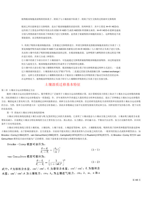
土壤溶质迁移基本特征第三章土壤水分运动参数确定方法随着土壤水分运动定量研究的深入,数学模型已广泛被用于土壤水分运动的模拟计算,而计算精度很大程度上取决于土壤水分运动参数的准确性。
因此准确估计土壤水分运动参数成为一项基础]:作。
多年来国内外学者通过大量的理论分析和实验验证,提出了多种确定土壤水分运动参数的方法,概括起来主要有两大类,即直接测定法和间接推求法。
两种方法各具特点和优势,但总的研究趋势是寻求利用简单实验获得土壤水分运动参数的方法。
低渗透介质中一维溶质运移实验研究
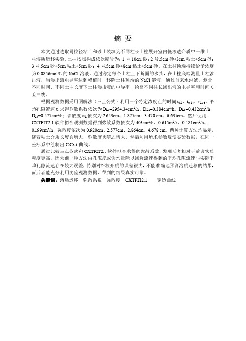
摘要本文通过选取同粒径粘土和砂土装填为不同柱长土柱展开室内低渗透介质中一维土柱溶质运移实验。
土柱按照构成依次编号为:1号.10cm砂;2号.5cm砂+3cm粘土+5cm砂;3号.5cm砂+5cm粘土+5cm砂;4号.5cm砂+8cm粘土+5cm砂。
在土柱顶端持续给予浓度为0.0856mol/L的NaCl溶液,通过稳定每个土柱上下断面的水头,在土柱底端测量土柱渗出液,当渗出液电导率达到峰值时,移除土柱顶端的NaCl溶液,通过自来水淋滤,测量不同时间、不同土柱长度下土柱渗出液的电导率,绘出不同柱长渗出液的电导率和时间关系曲线。
根据观测数据采用图解法(三点公式)利用三个特定浓度点的时间t0.5、t0.84、t0.16,平均孔隙流速u求得弥散系数依次为D L1=2954.34cm2/h、D L2=0.384cm2/h、D L3=0.432cm2/h、D L4=0.577cm2/h;弥散度αL依次为2.653cm、1.825cm、3.470 cm、6.635cm。
然后使用CXTFIT2.1软件拟合观测数据得到弥散系数依次为403cm2/h、0.615m2/h、0.181cm2/h、0.199cm2/h,弥散度依次为0.920cm、2.577cm、2.864cm、4.678 cm。
两种计算方法均显示,随着粘土介质长度的增大,弥散度也随之增大。
然后利用所求参数反演实验数据,在同一坐标系中绘制出C/C0-t曲线。
通过比较三点公式和CXTFIT2.1软件拟合求得的弥散系数,发现后者相对于前者实验精度更高,因为前一种方法由孔隙度或含水量除以渗透流速得到的平均孔隙流速与实际平均孔隙流速存在较大误差,特别对细粒介质的误差很大,不能准确地预测溶质迁移的结果,而后者能充分利用实验观测数据,得到的结果真实可靠。
关键词:溶质运移弥散系数弥散度CXTFIT2.1 穿透曲线ABSTRACTIn this thesis, we have did the solute transport experiments and the leaching experiments in four soil columns with the same particle size and different column lengths. According to the composition of soil columns , soil samples are numbered as: The 1st. 10cm sand; the 2nd. 5cm sand+3cm soil+5cm sand; the 3rd . 5cm sand +5cm soil +5cm sand; the 4th.5cm sand +8cm soil+5cm sand. By stabilizing the soil columns’ hydraulic head , we use the NaCl solution t o simulate the soluble contaminants . Then we get a series of data by measuring the electrical conductivity in the soil columns with the changeable time .By the data we obtained, we draw the BTC.We take two methods to get the dispersion coefficient :The first way is to make the use of three specific concentration point time t0.5,t0.84,t0.16 and the average pore velocity to calculate it. Then we get the dispersion coefficient are D L1=2954.34cm2/h, D L2=0.384cm2/h, D L3=0.432cm2/h, D L4=0.577cm2/h, the dispe rsivity αL are 2.653cm, 1.825cm, 3.470 cm, 6.635 cm. The other way is to enter experimental data into the CXTFIT2.1 programme to obtain dispersion coefficient , and using the inverse technique to get another experimental data. Then we get the diffusion coefficient are 403cm2/h, 0.615m2/h, 0.181cm2/h, 0.199cm2/h, the dispersivity αL are 0.920cm, 2.577cm, 2.864cm, 4.678cm.As shown from the two calculation methods, the dispersivity increases as the soil column length increase. Then analyze the simulation results, the calculated parameters inversion values and the real values. Then we draw the C/C0—t curve in the same coordinate system .For the reason of making full use of the experimental observations, the CXTFIT 2.1 program got a higher accuracy when it is compared with the former way. And we also found that it has a great difference between the D L obtained by the average pore velocity we used and the actual average velocity . The results obtained by porosity and average pore velocity we used were inexact. If we take them as the same one ,we will make a great mistake, especially for fine medium ,so it can’t reflect the results of solute transport accurately.Keywords: s olute transport dispersion coefficient dispersivity CXTFIT2.1 program the break through curve(BTC)目录第一章绪论............................................................................................................................ - 4 - 第二章国内外研究进展........................................................................................................ - 6 - 第一节国内外研究进展.................................................................................................. - 6 - 第二节研究中的问题...................................................................................................... - 7 - 第三节本文的研究思路和内容...................................................................................... - 7 - 第三章实验方案.................................................................................................................... - 8 - 第一节实验仪器.............................................................................................................. - 8 - 第二节实验步骤.............................................................................................................. - 9 - 第三节实验物理参数的测定........................................................................................ - 13 - 第四节实验成果分析方法............................................................................................ - 15 - 第五节实验成果分析.................................................................................................... - 21 - 第四章结论及建议................................................................................................................ - 29 - 第一节本实验得出的结论............................................................................................ - 29 - 第二节实验误差分析及不足........................................................................................ - 29 - 第三节对后续实验的建议............................................................................................ - 30 - 致谢.......................................................................................................................................... - 30 - 参考文献.................................................................................................................................. - 32 -第一章绪论我国是一个水资源相对短缺的国家,人均水资源占有量仅为世界人均占有量的四分之一,水资源己成为我国经济、社会和环境可持续发展的关键制约因素。
水及溶质在有大孔隙的土壤中运移机制研究进展
的实验 ; 另一类 是古有 大孔 晾 土壤的水 流实 验 . 11 确定大 孔豫大 小分布 的 实验 . 确定大孔 晾大小 分 布 , 了较早采用 的水 的吸 附. 吸 附 、 除 解 N的 吸附 和 H 的 注人 方 法外 , 包 括 以下 7 还 种实 验方法 .
冯 杰, 郝振纯
2嗍 ) 1 ( 河海大学水蟹源开 发利用国家专业 实验室 . 苏 南京 江
捕要: 综述 了水及溶质在有大孔隙的土壤 中运移的实验和模型研 究进展 , 出: 指 夸后应通过大量的 室内外实验和改进观测方法来获得大量的数据资料 , 从定性和定量两方面采研究大孔隙流; 只有在 参数的测定和一盛量的确定技 术解班以后 , 模型才能得到完善 而达到实用的程度 ; 为解决太孔隙系 统流动过程 中的高度非线性和非稳定性 问题 , 需要新的模拟方法和数值计算方法; 夸后模拟研 究的
分布 . 染色方 法确定 太孔 晾分布 的缺 点是 : 用 土样 的挖取 是破 坏性 的 , 试验 结果 不 能在 同一地 点重复获得 ; 虽
然能看到太孔睬的空问分布, 但不能准确确定太孔晾的太小, 也不能确定溶质浓度的差异.m a O o 等 用荧光
收薯日期:0卜0 6 20 卜1 暮盒璜 目: 国家 自拣科学基叠 资助项 目( r 搠强 ) 作者筒介: 冯燕( 7 一 ) , 12 男 山东聊城^ . 博士 , 水文学及水赘潭专盟 . 从事水文 物理规 律研究
a 土柱浸泡的方法. . 将非扰动土柱放人石蜡I4 3J ,和聚酯树脂或环氧树脂【 中浸泡, 5 】 观察从浸泡过的土柱
中取 出的土壤断面.et[采用人工计数方法确定土壤的大孔晾度 ;fHl掣 在紫外线光下对土壤断面 DxrJ e3 v_ l 】 皿
第6章 土壤溶质与溶质运移
2. 分子(或离子)扩散 分子(或离子)扩散是指气相或液相内部由于分子的不 规则热运动即布朗运动和分子之间的相互碰撞而引起 的质量运移。 土壤溶液中的溶质浓度并不总是均匀的。只要浓度梯度 存在,分子扩散就会发生。分子扩散导致溶质从浓度 高的区域向浓度低的区域运动,从而使溶液浓度趋于 均匀。在一个静止的水体中,由于分子扩散而引起的 溶质质量运移通量可由Fick’s first law描述。在一维条 件下,它可表达为:
土壤溶质研究范围: 土壤溶质 肥料运移: N(NO3-、NH4+)、P(H2PO4-)、K+ 等 盐分运移: Cl- 、 CO3 2 - 、 SO42- 、Br- 、Ca2+ 、 Mg2+ 、 Na+等 污染物迁移: 非水相流体(Light and Dense non-aqueous phase liquids (LNAPLs and DNAPLs): 汽油, TCA、甲苯、煤焦油等 小生物实体(Biologic entities ): 病毒(viruses), 细菌(bacteria) 辐射元素(Radioactive elements): 镭(Ra)、铍(Be)、氦(He)等天 然放射性物质 重金属元素 : 汞(Hg)、铅(Pb)、铜(Cu)等 柴油, 润滑油、碳氢化合物; 溶剂、工业洗涤剂、三氯乙烯TCE、四氯乙烯PCE、三氯甲烷
J dis = − Ddis ∂c ∂z (4.66)
目前很难在实验室或田间试验中明确地区分开分子(离 子)扩散和机械弥散的影响,因此一般将机械弥散和 分子扩散这两种现象合并而统称为水动力弥散现象。 机械弥散系数和分子扩散系数合并为一个参数即水动 力弥散系数或扩散弥散系数DH:
DH = Ddif + Ddis
土壤溶质迁移求解思路

在土壤中,溶质分子扩散符合菲克定律,即ds mc J D x∂=-∂ 式中ds J 为土壤中溶质分子扩撒通量,m D 是在土壤中分子扩散系数.由于受土壤含水量、空隙弯曲度等因的影响,土壤中分子扩散系数比自由水中小。
一般把在土壤中溶质扩散系数表示为含水量的函数,而与土壤溶质浓度无关,即b m w D D ae θ=式中:由于土壤中存在着大小不一、形状各异的的空隙,水溶液在其中流动过程中,每个空隙中的流苏大小和方向各不相同,使溶液分散并扩大运移范围的现象称之为机械弥散.机械弥散所引起俄溶质迁移通量表示为h hc J D x∂=-∂ 式中h J 为土壤中溶质分子扩撒通量,h D 是在土壤中分子扩散系数。
通常机械弥散系数可以表示为空隙流速的函数,即nh D vλ=式中:λ是弥散度,n 是经验系数,v 是空隙平均水流速度。
一般认为机械弥散系数与平均空隙水流速度成一次方程正比,这样经验系数n =1,弥散度的大小取决于水分通量和溶质对流弥散通量的平均尺度大小,一般来说扰动土条件下,λ的值为0.5 到2cm 之间机械弥散和分子扩散作用在土壤中都引起溶质迁移,但因围观流速不以测量,弥散作用与扩散作用也很难区别,同时两者的所引起的溶质迁移通量表达式的形式基本相同。
所以在实际中长把两种作用联合考虑,并称之为水动力弥散。
同样把分子扩散系数和机械弥散系数叠加起来,称之为水动力弥散系数。
因此水动力弥散作用是个别分子在空袭中运动及所发生的一切物理和化学作用的宏观表现。
根据水动力弥散定义以及分子扩撒和机械弥散间的关系,可把水动力弥散引起的土壤溶质迁移通量表示为:lh lh cJ D x∂=-∂式中:lh J 是水动力弥散引起的溶质通量,lh D 水水动力弥散系数,nb lhw D D ae vθλ=+土壤水是土壤溶质迁移的载体,溶质可以随着土壤水分整体运动而迁移,这种迁移过程称之为对流。
由于对流作用引起的土壤溶质迁移通量与土壤水分通量和水溶液浓度与关,可表示为wc w J J c =式中:wc J 是对流引起的溶质通量,w J 是土壤水分通量.因此以液态形式迁移的土壤溶质通量可表示为wc lh cJ J D x∂=-∂惰性非饱和吸附性溶质的迁移:()()((,))w lh c c J c D v t x x xθθ∂∂∂∂=-∂∂∂∂ 上式描述了非稳定流情况下的土壤溶质迁移过程.对于稳定流情况()()w lh cc J c D t x x xθθ∂∂∂∂=-∂∂∂∂ 上述方程可进一步化简为22v c c cD v t x x∂∂∂=-∂∂∂ 式中:/vlh D D θ=,qv θ=初始和边界条件:000(,0)(0,)(0)(0,)0()(,)0ic x c c t ct t c t t t c t x=⎧⎪=<≤⎪⎪⎨=>⎪∂∞⎪=⎪∂⎩其解析表达式为000000()(,)(0)(,)()(,)(,)()i i i i c c c A x t t t c x t c c c A x t c A x t t t t +-<≤⎧=⎨+--->⎩1/21/211(,)[]exp()[]22()22()v v v x vt vx x vtA x t erfc erfc D t D D t -+=+ 22().lh c c c D q t x xθθ∂∂∂=-∂∂∂一维水平非饱和水动力参数的测定原理: 1一维水平非饱和溶质迁移模型()()((,))w lh c c J c D v t x x x θθ∂∂∂∂=-∂∂∂∂ ()..((,))()w w lh c c J c c J D v t x x x xθθ∂∂∂∂∂=-+∂∂∂∂∂ 由于wc w J J c =()wJ k s xθ=∂∂ ()().()k D C θθθ=,m S ϕ=-()md c d θθϕ=()w J D x θθ∂=-∂()wcJ D c xθθ∂=-∂故由()..((,))()w wlh c c J c c J D v t x x x xθθ∂∂∂∂∂=-+∂∂∂∂∂ 可得()..(())..(())()lh D c c D c c c x x D t t x x x x θθθθθθθ∂∂-∂∂-∂∂∂∂∂∂+=-+∂∂∂∂∂∂()..(())..(())()lh D c c D c c c x x D t t x x x xθθθθθθθ∂∂∂∂∂∂∂∂∂∂+=++∂∂∂∂∂∂ ..(())()[()]lh cc c c D D c D tt x x x x x xθθθθθθθ∂∂∂∂∂∂∂∂+=++∂∂∂∂∂∂∂∂222()..(())..(,).().)()lh lh D c c D c c c D v c x x D t t x x x xθθθθθθθθ∂∂∂∂∂∂∂∂∂∂∂+=+++∂∂∂∂∂∂其边界条件为 00(0,)(,0)(,)(0,)(0,0)0(,0)(,)a b a a bt x t x t x l c c t x c ct t x c t t x c t xθθθθθθ⎧⎪==⎪==⎪⎪=>⎪⎪==⎨⎪=<≤=⎪=>=⎪⎪∂∞⎪⎪∂⎩由一维土壤溶质迁移方程可知,方程中待求参数为水动力弥散系数(,)lh D v θ和水分扩散系数()D θ又由于nb lh w D D ae vθλ=+msD D )()(0θθθ= )(0)(θθβθ--=se D D 120.5()11mmr r s s r s r D D θθθθθθθθθ⎧⎫⎡⎤⎛⎫⎛⎫--⎪⎪⎢⎥=--⎨⎬ ⎪ ⎪--⎢⎥⎝⎭⎝⎭⎪⎪⎣⎦⎩⎭因而只要确定水动力弥散系数计算公式nb lh w D D ae v θλ=+中的自由水中分子扩散系数wD 以及指数a 、b ,机械弥散公式中的弥散度λ,和经验系数n ,以及空隙平均水流速度v ;还有水分扩散系数公式之一msD D )()(0θθθ=中的饱和扩散率0D 以及指数m ,那么就可以求得任意时刻各点的含水率以及溶质浓度分布。
土壤水与溶质的运移
土壤水与溶质的运移Contents5.0 Introduction5.1 Classifying and determining of soil water土壤水的类型划分及土壤水分含量的测定5.2 Energy status of soil water土壤水的能态5.3 Soil water movement土壤水的运动5.4 Solute transportation in soils土壤中的溶质运移Soil water土壤水是土壤的最重要组成部分之一;在土壤形成过程中起着极其重要的作用,在很大程度上参与了土壤内进行的许多物质转化过程:矿物质风化、有机化合物的合成和分解等;作物吸水的最主要来源;自然界水循环的重要环节;非纯水,而是稀薄的溶液,溶有各种溶质,还有胶体颗粒悬浮或分散其中。
Principal sources of soil water●Precipitation——Rain, snow, hail(雹); fog, mist(霜)●Ground water——lateral movement from upslope, upward movement from the underlying rock strata.precipitation Surface devoid of vegetationReachdirectly Vegetated surfaceinterceptedcanopyCanopy throughfall andstemflow atmosphereevaporation infiltration Run offSoil waterDrainage and lostEvapotraspirationThe composition of soil waterSoil water contains a number of dissolved solid and gaseous constituents,many of which exist in mobile ionic form,and a variety of suspended solid components.Base cations(Ca2+, Mg2+, K+, Na+, NH4+)PrecipitationMineral weatheringOrganic matter decomposition Lime and fertilizersourcesH+——a measure of acidity (pH)●CO2Atmosphere ——dissolved in precipitation Soil air ——produced in soil respirationH2O + CO2H2CO3H++ HCO3-Unpolluted rain water: pH>5.6Soil water: pH <5.0●Industrial and urban emission●Organic acids derived from decaying organic material●Released by plants in exchange for nutrient base cations major sourceIron and aluminiumMajor sourcesmineral weatheringacid rainMajor formFe2+, Al3+ionssoluble organic-metallic complexesSoluble anionsNO3-, PO43-Cl-, SO42-HCO3-Mineralisation processesFertilizersAtmosphere sourcesMineral weatheringDissolved organic carbon (DOC) Pollutants (heavy metals et al.)Suspended constitutions☐Small particles of mineral and organic material ☐Often result in discoloration(变污)and increased turbidity(混浊度)of soil water.第一节土壤水的类型划分及土壤水分含量测定Classifying and determining of soil water 一、土壤水分类型及有效性Soil water types and availability土壤水分研究方法能量法数量法从土壤水分受各种力作用后自由能的变化研究水分的能态和运动、变化规律。
- 1、下载文档前请自行甄别文档内容的完整性,平台不提供额外的编辑、内容补充、找答案等附加服务。
- 2、"仅部分预览"的文档,不可在线预览部分如存在完整性等问题,可反馈申请退款(可完整预览的文档不适用该条件!)。
- 3、如文档侵犯您的权益,请联系客服反馈,我们会尽快为您处理(人工客服工作时间:9:00-18:30)。
土壤系统中溶质运移研究博士研究生:石 辉学科、专业:土壤学研究方向:土壤溶质运移导 师:邵明安研究员为了满足日益增长的人口对粮食的需求,农用化学物质被广泛使用,这些物质可通过各种渠道进入土壤,因此研究土壤中农用化学物质的迁移、转化对于防止环境污染和促进农业持续发展有着重要的意义。
本文在对土壤溶质运移理论分析的基础上,采用土柱实验、田间实验以及计算机模拟研究土壤系统中溶质的运移过程,得到以下主要结论:1.通过分析土壤溶质运移与化学色谱之间的相似性,利用化学色谱理论分析了土壤溶质穿透曲线的形状,以及塔板理论模拟溶质运移的穿透曲线。
发现穿透曲线的形状主要由溶质在固体土粒与溶液中浓度的吸附等温线来决定,对于凸型分配函数,表现为前缘陡峭、后缘“拖尾”的“拖尾”型穿透曲线;对于凹型分配函数,表现为前缘“伸舌”、后缘陡峭的“伸舌”型穿透曲线。
对于非反应型溶质理论上应当保持对称的高斯型穿透曲线,但在实际土壤中由于不动水体的存在,穿透曲线也表现出前缘陡峭、后缘拖尾的“拖尾”型穿透曲线。
根据塔板理论认为土柱由理想形态的一系列小塔板所组成,忽略弥散作用,利用质量守恒定律可得到描述溶质运移的塔板模型]21)2e x p (21[210N M M e r f c N N M M e r f c c c ++-= (1)该模型与溶质运移的CDE 方程解具有一定的相似性,但由于忽略了弥散作用,其估计 浓度低于CDE 方程。
2.研究表明,在一般情况解析解第二项的贡献较小(<4%),可以省略。
对CDE 方程 省略第二项后的解析解进行了详细分析,通过误差函数的逆运算得到下述公式D utx Ce arcerf t 2)21(-=- (2) 对于穿透曲线则有tD uD L22-=ξ (3)这样可利用ζ与t 线形关系的斜率、截距估计CDE 参数D 、R 值。
实验结果证实该方 法与常用CXTFIT 拟合结果一致。
当Ce 按照边界层定义一个固定值时,式(2)则为边界 层与时间的关系。
对于边界层,定义其相对浓度为3‰时拟合参数与CXTFIT 结果一致。
测定穿透曲线费时费力,由式(2)可利用任意两个时刻的Ce (x 1,t 1),Ce (x 2,t 2)估计参 数。
3.对薄层土壤溶质运移的可动水体与不可动水体模型进行了研究。
发现对于薄层土壤 在忽略弥散的作用下,其溶质运移穿透可用式(4)表示VV e e C C )1)(1()1(0)1(1φξφφξξξ+--+--+=- (4) 式(4)表明,可将薄层土壤溶质运移分为二个阶段。
初始阶段,由于ξ和V 较小,式(4)的第一项较小,因而对浓度影响不大;而在后期阶段,第二项的数值变小,浓度主要由第一项决定,但第二项数值减小的幅度较慢。
用土柱实验进行了验证。
4.研究了田间NO 3-N 的时空变化。
发现NO 3-N 在垂直方向上可分为0-60cm , 60-140cm ,140-200cm 三个层次,层次间NO 3-N 的含量达到显著差异。
在水平方向上,NO 3-N 的变异远远大于土壤水分的变异。
NO 3-N 随时间的变化主要表现在气候因素对其的影响。
随着降雨量的增加,0-60cm 土层中的NO 3-N 表现出减少趋势;而60-140cm 在降雨量小于50mm 时随降雨量的增加NO 3-N 含量增加,而大于50mm 时随降雨量的增加而减少;140-200cm NO 3-N 基本不变。
这可能有在低降雨量的情况下将上层NO 3-N 淋溶进入中层,引起中层的NO 3-N 增加;而降雨量大时,降雨可将NO 3-N 淋入下层,导致中层NO 3-N 降低。
NO 3-N 的产生与温度关系密切,随温度的增加,0-60 cm 土层的NO 3-N 增加,而下两层则变化平缓。
这主要由于NO 3-N 在表层产生,随温度增加,硝化作用增强,NO 3-N 生成增加;而土壤下层,土壤温度本身变化较小且非NO 3-N 的主要生成区,因而随温度变化较小。
5.关于土壤溶质运移的研究,主要是在饱和条件下进行的,但实际化学物质是在非饱和情况下运移的,与土壤水分运动存在耦合。
本文介绍了土壤水分、溶质耦合运动的基本方程,所采用土壤水分、基质势、导水率关系以及所采用的边界、初始条件,模拟非饱和土壤的水分、溶质耦合运动。
模拟结果表明,水分的湿溶锋与溶质锋在非饱和情况下并不重合。
在对田间情况进行简化后,模拟田间NO 3-N 与水分运动情况,结果在趋势上与实测值具有相似性,但由于土壤的非均质性、边界条件的选择等因素使预测值与测定值存在一定的偏差。
关键词:溶质运移 塔板理论 对流——弥散方程(CDE ) 可动与不可动水体模型(MIM ) NO 3-N 水分与溶质耦合运动Solute Transport in SoilsIn order to meet the demand for food of the increasing population, agri-chemicals are widely used. Agri-chemicals enter soils by many ways, solute transport and its transfer in soils have great significance for prevention of environmental pollution and maintenance of sustainable agriculture. In this paper, based on theoretical analysis of solute transport in soils, soil column experiment, and field experiment and computer simulation technique were used to study solute transport in soils. Meanwhile, a method for fertilization application localized compaction dime, which can prevent leaching of N fertilizer and improve fertilizer use efficiency, was presented. This is an example of application for the theoretical achievements of solute transport. The results are as the fellows.1.By analyzing the similarity between solute transport in soil and chromatography in chemistry, shapes of Breakthrough Curve (BTC) and simulation soil solute transport by using chromatography were conducted. The shape of BTC is mainly determined by adsorption isotherm between soil solid particle and soil solution. For convex function, there is “pulling tail ” BTC that the front part of BTC is high and steep and the rear part of BTC is “pulling tail ”. For concave function, there is “stretching tongue ” BTC that the front part of BTC is “stretching tongue ” and the rear part of BTC is high and steep. For non-reactive solute, BTC is “pulling tail ” type because there is immobile water in field soils. According to the plate theory, the soil column was formed by a series plates and the plate model is obtained by neglecting dispersion:]21)2exp(21[210N M M erfc N N M M erfc c c ++-= (1)This model has same tendency as the analytical solution of CDE, but the estimation result was less accurate than CDE due to neglecting dispersion.rge amount of research indicated that under normal condition, the contribution of the second term of analytical solution of CDE is relatively small (<4%) and then can be neglected. For the analytical solution of neglecting the second term, the following formula can be acquired through inverse operation of the error functionD ut x Ce arcerf t 2)21(-=- (2 ) For BTC, which ist D u D L 22-=ξ (3 ) So the parameters of D and R can be estimated by the slope and intercept of linear relationship between ξ and t . The estimated parameters from experimental result by intercept method were similar as by CXTFIT method. When the relative concentration Ce was defined as a constant for a boundary layer, Eq.(2) shows the relationship between the position of boundary layer x and time t .When Ce was defined as 3‰ in the boundary layer, the results were as same as CXTFIT. Meanwhile, the parameters of CDE can be estimated by any two point Ce(xl, tl) and Ce(x2, t2) through Eq.(2).3. Solute transport using MIM model in a thin-layer soil was carried out and the results showed that the effluent concentration can be expressed by Eq.(4) of dispersion is neglectingVV e e C C )1)(1()1(0)1(1φξφφξξξ+--+--+=- (4) Eq.(4) indicated that solute transport in a thin-layer soil can be divided into two stags. At the initial stage, ξand V was relatively small. So that the first term is small and it has little contribution to effluent concentration. In the second stage, the value of second term becomes smaller; the first term is dominant.4. The temporal and spatial variability of NO 3-N in field condition was studied. The results showed that the change of NO 3-N with depth could be divided into three layers, i.e. 0-60cm, 60-140cm, and 140-200cm. For the horizontal level, variation of NO 3-N is much larger than that of soil moisture. Changes of NO 3-N content with time mainly reflect the effect of climate. NO 3-N content in 0-60cm decreased with the increase of rainfall. In 60-140cm, NO 3-N increased when precipitation was less than 50mm but decreased when precipitation was greater than 50mm. NO 3-N in 140-200cm has little variation. The reasons are under the condition of smaller rainfall, NO 3-N in the upper layer is leached into the middle layer, thus NO 3-N in the middle layer is increased. When the rainfall is larger, the NO 3-N in the middle is leached into lower layer, so the amount in middle layer becomes smaller. The NO 3-N content was closely related with temperature. With the increase of temperature, NO 3-N in 0-60cm layer is increased, but other layers have small change. NO 3-N is formed mainly in top layer; nitrification is enhanced with the increase of temperature, thus NO 3-N content in upper layer raised. Between two lower layers, the change of temperature is small, so relative varieties of NO 3-N are very little,5. Most solute transport in soils was studied in a saturated condition, but agri-chemicalstransport often happened in unsaturated condition. Solute transport usually couples with soil water movement. Based on the mechanism of soil moisture and solute transport, and relationship among soil moisture, matric potential and hydraulic conductivity, the movement of soil moisture coupling with solute was simulated for specified boundary and initial conditions. The results showed that the wetting front was not coinciding with the solute front. After simplifying rainfall condition, the simulation results of NO 3-N and soil moisture showed same change trends as measurement but there existed some deviation because of soil nonhomogenity and boundary condition.Keywords: Solute transport, Plate theory, Convection-dispersion equation (CDE), Mobile and immobile model (MIM), NO 3-N, Temporal and spatial variety, Movement of soil moisture coupled with solute transport。