图像缩放算法比较分析(IJIGSP-V5-N5-7)
基于改进自组织映射和BP神经网络的高速图像压缩.(IJIGSP-V6-N5-4)
High-speed Image compression based on the Combination of Modified Self-organizing Maps and Back-Propagation Neural Networks
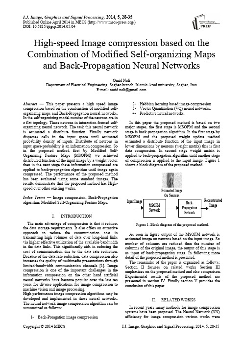
Omid Nali Department of Electrical Engineering, Saghez branch, Islamic Azad university, Saghez, Iran E-mail: omid.nali@ Abstract — This paper presents a high speed image compression based on the combination of modified selforganizing maps and Back-Propagation neural networks. In the self-organizing model number of the neurons are in a flat topology. These neurons in interaction formed selforganizing neural network. The task this neural network is estimated a distribute function. Finally network disperses cells in the input space until estimated probability density of inputs. Distribute of neurons in input space probability is an information compression. So in the proposed method first by Modified SelfOrganizing Feature Maps (MSOFM) we achieved distributed function of the input image by a weight vector then in the next stage these information compressed are applied to back-propagation algorithm until image again compressed. The performance of the proposed method has been evaluated using some standard images. The results demonstrate that the proposed method has Highspeed over other existing works. Index Terms — Image compression; Back-Propagation algorithm; Modified Self-Organizing Feature Maps. I. INTRODUCTION 2- Hebbian learning based image compression 3- Vector Quantization (VQ) neural networks. 4- Predictive neural networks. In this paper the proposed method is based on two major stages, the first stage is MSOFM and the second stage is back-propagation algorithm. In the first stage by MSOFM and the proposed weight update method estimated a distribute function of the input image in lower dimensions by neurons (weight matrix) this is first data compression. In second stage weight matrix is applied to back-propagation algorithm until another stage of compression is applied to the input image. Figure 1 shows a block diagram of the proposed method.
评估及比较视频压缩运动估计算法(IJIGSP-V5-N10-2)
I.J. Image, Graphics and Signal Processing, 2013, 10, 9-18Published Online August 2013 in MECS (/)DOI: 10.5815/ijigsp.2013.10.02Evaluation and Comparison of Motion Estimation Algorithms for Video CompressionAvinash Nayak and Bijayinee BiswalAjay Binay Institute of Technology, Odisha, Indianayak.av@S. K. SabutM.S. Ramaiah Institute of Technology, Bangalore, Indiasukanta207@Abstract — Video compression has become an essential component of broadcast and entertainment media. Motion Estimation and compensation techniques, which can eliminate temporal redundancy between adjacent frames effectively, have been widely applied to popular video compression coding standards such as MPEG-2, MPEG-4. Traditional fast block matching algorithms are easily trapped into the local minima resulting in degradation on video quality to some extent after decoding. In thi s paper various computing techniques are evaluated in video compression for achieving global optimal solution for motion estimation. Zero motion prejudgment is implemented for finding static macro blocks (MB) which do not need to perform remaining search thus reduces the computational cost. Adaptive Rood Pattern Search (ARPS) motion estimation algorithm is also adapted to reduce the motion vector overhead in frame prediction. The simulation results showed that the ARPS algorithm is very effective in reducing the computations overhead and achieves very good Peak Signal to Noise Ratio (PSNR) values. This method significantly reduces the computational complexity involved in the frame prediction and also least prediction error in all video sequences. Thus ARPS technique is more efficient than the conventional searching algorithms in video compression.Index Terms— Video Compression, Motion Estimation, Full Search Algorithm, Adaptive, Rood Pattern Search, Peak Signal to Noise RatioI.I NTR ODUC TIONImportance of digital video coding has increased significantly since the 90s when MPEG-1 first came to the picture. Compared to analog video, video coding achieves higher data compression rates without significant loss of subjective picture quality which eliminates the need of high bandwidth as required in analog video delivery to a large extent. Digital video is immune to noise, easier to transmit and is able to providea more interactive interface to the users [1]. The specialized nature of video applications has led to the development of video processing systems having different size, quality, performance, power consumption and cost.A major problem in a video sequence is the high requirement of memory space for storage. A typical system needs to send dozens of individual frames per second to create an illusion of a moving picture. For this reason, several standards for compression of the video have been developed. Each individual frame is coded to remove the redundancy [2]. Furthermore, between consecutive frames, a great deal of redundancy is removed with a motion compensating system. Motion estimation and compensation are used to reduce temporal redundancy between successive frames in the time domain.A number of fast block matching motion estimation algorithms were considered in different video coding standards because massive computation were required in the implementation of exhaustive search (ES). In order to speed up the process by reducing the number of search locations, many fast algorithms have been developed, such as the existing three-step search (TSS) algorithm [3]. The Three Step Search method is based on the real world image sequence’s characteristic of centre-biased motion vector distribution, and uses centre-biased checking point patterns and a relatively s mall number of search locations to perform fast block matching. In order to reduce the computational complexity for motion estimation and improve the reliability of the image sequences for super-resolution reconstruction, an effective three-step search algorithm is presented. Based on the center-biased characteristic and parallel processing of the motion vector, the new algorithm adopts the multi-step search strategy [4].A simple, robust and efficient fast block-matching motion estimation (BMME) algorithm called diamond search, which employs two search patterns. The first pattern, called large diamond search pattern (LDSP), comprises nine checking points from which eight points surround the center one to compose a diamond shape. The second pattern consisting of five checking points forms a smaller diamond shape, called s mall diamond search pattern (SDSP).10Evaluation and Comparison of Motion Estimation Algorithms for Video CompressionA simple fast block-matching algorithm (BMA), called adaptive rood pattern searches (ARPS), which consist of two sequential search stages: 1) initial search and 2) refined local search. The initial search is performed only once at the beginning for each MB. This removes unnecessary intermediate search. For the initial search stage, ARP is proposed, based on the available motion vectors (MVs) of the neighboring MBs. In the next stage, a unit-size rood pattern (URP) is exploited repeatedly, and unrestrictedly, until the final MV is found. In this paper we have evaluated the following four algorithms: Exhaustive Search (ES), Three Step Search (TSS), Diamond Search (DS), and ARPS.II.METHODSIn a conventional predictive coding [5-6], the difference between the current frame and the predicted frame is encoded. The prediction is done using any of the BMA. BMA are used to estimate the motion vectors. Block-matching consumes a significant portion of time in the encoding step.A.Block matching algorithmBlock matching algorithm (BMA) is widely used in many motion-compensated video coding systems such as H.261 and MPEG standards to remove interframe redundancy and thus achieve high data compression [7, 8]. The process of block-matching algorithm is illustrated in Fig.1. Motion estimation is performed on the luminance block in which the present frame is matched against candidate blocks in a search area on the reference frame for coding efficiency. The best candidate block is found and its motion vector is recorded. Typically the input frame is subtracted from the prediction of the reference frame, thus interframe redundancy is removed and data compression is achieved. At receiver end, the decoder builds the frame difference signal from the received data and adds it to the reconstructed reference frames. This algorithm is based on a translational model of the motion of objects between frames [9].Reference Frame Current FrameFigure 1. Block-matching motion estimationThe block-based motion vectors can be estimated by using block matching, which minimizes a measure of matching error. The destination of motion estimation is to find macro-block (MB) in the reference frame which has the smallest difference from the MB in the current frame. The difference is denoted by Sum of Absolute Difference (SAD), as shown in equation (1). The SAD is the most popular matching criteria used for block-based motion estimation.1100(,)(,)(,),,N Ni jS A D m n c i j s i m j n m nωω−−===−++≤≤∑∑ (1)Where SAD (m, n) is the distortion of the candidate block at search position (m, n), {c (x, y) | 0 ≤ x ≤ N −1, 0≤ y ≤ N −1} means current block data, {s (x, y)| −w ≤ x ≤ w + N −1,−w ≤ y ≤ w + N −1} stands for search area data, the search range is [-w, w], the block size is N×N. (2w+1) 2 motion vectors to be checked .Consider a block of pixels of size N × N in the reference frame, at a displacement of, where I and j are integers with respect to the candidate block position. SAD makes the error values as positive, but instead of summing up the squared differences, the absolute differences are summed up. The SAD criterion shown in equation (1) requires N2computations of subtractions with absolute values and additions N2 for each candidate block at each search position. The absence of multiplications makes this criterion computationally more attractive and facilitates easier hardware implementation. Peak-Signal-to-Noise-Ratio (PSNR) given by equation (2) characterizes the motion compensated image that is created by using motion vectors and macro blocks from the reference frame.Γ=Round |MV������⃗predicted|= Round(y)]MV(x)[MV predicted2predicted2+(2) Where MV predicted(x)and MV predicted(y) are the horizontal and vertical components of the predicted MV, respectively. Operator “Round” performs rounding operation, which takes the nearest integer value of the argument.B.Exhaustive search (ES) algorithmThe exhaustive search (ES) algorithm also known as Full Search is the most computationally expensive block matching algorithm. This algorithm calculates the cost function at each possible location in the search window. It gives the highest PSNR amongst any block matching algorithm by the best possible match [10]. Fast block matching algorithms try to achieve the same PSNR doing as little computation as possible. The obvious disadvantage to ES is that the larger the search window gets the more computations it requires.Search window (2w×2w)Reference frame Candidate frameFigure 2. Exhaustive Search Motion EstimationConsider a block of N × N pixels from the candidates frame at the coordinate position (r, s) as shown in Fig.2 above and then consider a search window having a range ±w in both the directions in the references frame, as shown. For each of the (2w + 1)2search position (including the current row and the current column of the reference frame), the candidate block is compared with a block of size N × N pixels, according to one of the matching criteria and the best matching block, along with the motion vector is determined only after all the (2w+1)2 search position are exhaustively explored. However, it is highly computational intensive.C.Three step search (TSS) algorithmKoga et al introduced this algorithm [11]. It became very popular because of its simplicity and also robust and near optimal performance. It searches for the best motion vectors in a coarse to fine search pattern. The algorithm has steps as described with the help of Fig.3.Step 1: An initial step size is picked. Eight blocks at a distance of step size from the centre are picked for comparison.Step 2: The step size is halved. The centre is moved to the point with the minimum distortion.Figure 3. Three Step Search proceduresThe point which gives the smallest criterion value among all tested points is selected as the final motion vector m.TSS reduces radically the number of candidate vectors to test, but the amount of computation required for evaluating the matching criterion value for each vector stays the same. TSS may not find the global minimum (or maximum) of the matching criterion; instead it may find only a local minimum and this reduces the quality of the motion compensation system. On the other hand, most criteria can be easily used with TSS [12].D.Diamond search (DS) algorithmBy exhaustively testing on all the candidate blocks, full search (FS) algorithm gives the global minimum SAD position which corresponds to the best matching block at the expense of highly computation. To overcome this defect, many fast block matching algorithms (BMAs) are developed such as diamond search [13].The proposed DS algorithm employs two search patterns as illustrated in Fig. 4.1 (a), (b) which are derived from the crosses (×) in Fig. 4. The first pattern, called large diamond search pattern (LDSP), comprises nine checking points from which eight points surround the centre one to compose a diamond shape (◊). The second pattern consisting of five checking points forms a smaller diamond shape, called small diamond search pattern (SDSP) [14,15]. The 13 crosses show all possible checking points within the circle.Figure 4. An appropriate search pattern support-circular areawith a radius of 2 pels. The 13 crosses show all possiblechecking points within the circle.(a) Large Diamond Search Pattern (b) Small Diamond SearchPatternFigure 4.1. Two search patterns derived from the last figure are employed in the proposed DS algorithm.Among the five checking points in SDSP, the position yielding the MBD provides the motion vector of the best matching block [16]. The DS algorithm is performed as follows:Step 1: The initial LDSP is centred at the origin of the search window, and the 9 checking points of LDSP are tested. If the MBD point calculated is located at the centred position, go to Step 3; otherwise, go to Step 2. Step 2: The MBD point found in the previous search step is re-positioned as the centre point to form a new LDSP. If the new MBD point obtained is located at the centre position, go toStep 3; otherwise, recursively repeat this step.Step 4: Switch the search pattern from LDSP to SDSP. The MBD point found in this step is the final solution of the motion vector which points to the best matching block.E.Adaptive rood pattern search (ARPS) algorithmAs we have observed, a small search pattern made up by compactly spaced search points is more suitable than a large search pattern containing sparsely spaced search points in detecting small motions, because only a small number of positions around the search window center arenecessary to be checked [17]. The speed and accuracy ofpattern-based search algorithms intimately depend on the size of the search pattern and the magnitude of the target MV. Therefore, it is highly desirable to use different search patterns according to the estimated motion behavior for the current block. This boils down to two issues required to be addressed: 1) How to pre-determine the motion behavior of the current block for performing efficient ME? 2) What are the most suitable size and shape of the search pattern(s)?Regarding the first issue, the current block’s motion behavior can be predicted by referring to its neighboring blocks’ MVs in the spatial domain. For the second issue, two types of search patterns are used. One is the adaptive rood pattern (ARP) with adjustable rood arm which is dynamically determined for each MB according to its predicted motion behavior. Note that ARP will be exploited only once at the beginning of each MB search [18]. Getting a good starting point for the remaining local search alleviates unnecessary intermediate search and reduces the risk of being trapped into local minimum in the case of long search path. A small, compact, and fixed-size search pattern would be able to complete the remaining local search quickly.1)Prediction of the target MVIn order to obtain an accurate MV prediction of the current block, two factors need to be considered: 1) Choice of the region of support (ROS) that consists of the neighboring blocks whose MVs will be used to calculate the predicted MV, and 2) A lgorithm used for computing the predicted MV.The spatial ROS is limited to the neighboring block(s) with four promising scenarios as shown in Fig.5. Type A covers all the four neighboring blocks, and +type B is the prediction ROS adopted in some international standards such as H.263 for differential coding of MVs. Type C is composed of two directly adjacent blocks, and type D has only one block that situates at the immediate left to the current block. Calculating the statistical average of MVs in the ROS is a common practice to obtain the predicted MV. The mean and median prediction has been tested in our experiments. Others (such as the weighted average) are either too complex in computation or involving undetermined parameters, they are therefore not considered in our work. Extensive experiments are performed with all four types of ROS and two types of prediction criteria- mean and median. Our experimental results show that these ROSs and prediction criteria yield fairly similar performance in terms of PSNR and the total number of checking points required. Therefore, we adopt the simplest ROS (i.e., type D) in our method, which has the least memory requirement, because only one neighboring MV needs to be recorded.TYPE A TYPE B TYPE C TYPE D Figure 5. Four types of ROS, depicted by the shaded blocks.The block marked by “○” is the current block. 2)2) Selection of search patternsAdaptive Pattern -For the Initial Search: The shape of our rood pattern is symmetrical, with four search points locating at the four vertices, as depicted in Fig.5. The main structure of ARP has a rood shape, and its size refers to the distance between any vertex point and the center point. The choice of the rood shape is first based on the observation of the motion feature of real-world video sequences. The rood shape pattern includes all the horizontal and vertical directions, so it can quickly detect such motion, and the searches will directly – ‘jump” into the local region of the global minimum.Secondly, any MV can be decomposed into one vertical MV component and one horizontal MV component. For a moving object which may introduce MV in any direction, rood-shaped pattern can at least detect the major trend of the moving object, which is the desired outcome in the initial search stage. Furthermore, ARP’s symmetry in shape not only benefits hardware implementation, but also increases robustness. It shows that even if the predicted MV could be inaccurate and its magnitude does not match the true motion very well, the rood-shaped pattern which takes all horizontal and vertical directions into consideration can still track the major direction and favor the follow-up refinement process. In addition to the four-armed rood pattern, it is desirable to add the predicted MV into our ARP because it is very likely to be similar to our target MV as shown in Fig.6. By doing so, the probability of detecting the accurate motion in the initial stage will be increased.Figure 6. Adaptive rood pattern (ARP)In our method, the four arms of the rood pattern are of equal length. The initial idea in deciding the ARP’s size is to make it equal to the length of the predicted MV (i.e., the MV of the immediate left block of the current block). That is, the size of ARP, Γ, isΓ=Round |MV������⃗predicted|= Round(y)]MV(x)[MV predicted2predicted2+(3) where MV predicted(x)and MV predicted(y) are the horizontal and vertical components of the predicted MV, respectively. Operator “Round” performs rounding operation, which takes the nearest integer value of the argument.Note that parameter Γ def ined in (2) involves square and square-root operations; thus, increasing difficulty on hardware implementation. Instead, we use only one of the two components of the predicted MV that has the larger absolute value (or magnitude) to determine the size of our ARP.That is:Γ=Max {MV predicted(x),MV predicted(y)} (4)From the mathematical standpoint, [19] the magnitude of MV’s component with larger absolute value is fairly close to the length of MV, and thus Equation (4) is a good approximation of measurement about motion magnitude. Experimental results show that the second definition of Γ using (4) is, in fact, slightly superior to the first one using (3) in terms of higher PSNR and less total number of checking points.The second method equation (4) for the rest of ARPS development was adopted. We observed that the chosen ROS (type D) is not applicable to all the leftmost blocks in each frame. For those blocks, we do not utilize any neighboring MVs, but adopted a fixed-size arm length of 2 pixels for the ARP, since this size agrees to that of LDSP which has fairly robust performance as reported in. Also, longer arm lengths are not considered because the boundary MBs in a frame usually belongs to static background.3)Fixed pattern-for refined local searchIn the initial search using ARP as described earlier, the adaptive rood pattern leads the new search center directly to the most promising area which is around the global minimum; thus, effectively reducing unnecessary intermediate searches along the search path. We use a fixed, compact and small search pattern to perform local refined search unrestrictedly for [MV (x) MV (y)] predicted identifying the global minimum. When a fixed pattern is used, the matching motion estimation (MME) point found in the current step will be re-positioned as the new search center of the next search iteration until the MME point is incurred at the center of the fixed pattern. Two types of most compact search patterns have been investigated in our experiments. One is the five-point unit-size rood pattern which is the same as SDSP used in DS, and the other is a 3x3 square pattern as shown in Fig.7 (a, b). This demonstrates the efficiency of using URP in local motion detection, and it is therefore adopted in our proposed method [20].(a) (b)Figure 7. Two fixed search patterns under consideration Image segmentation i s generally defined as the basic image processing that subdivides a digital image ),(yxfinto its continuous, di sconnect and nonempty subsetnffff,,,321, which provides convenience to extraction of attribute[3]. In general, Image segmentation algorithms are based on two basic principles[4]: the trait of pixels and the information in nearby regions. Most of segmentation algorithms are based on two characters of pixels gray level: discontinuity around edges and similarity in the same region. As is shown in Table I, there are three main categories in image segmentation[5]: A. edge-based segmentation; B. region-based segmentation; C. special- theory-based segmentation. And some sub-classes are included in the main categories too.III.S IMULATION R ESULTS AND D ISCUSSIONIn this paper we have evaluated the concepts of motion estimation, video compression, BMA using Exhaustive Search, Three-step Search, Diamond search and ARPS algorithm for 16 × 16 block size images of Chemical Plant, Toy Vehicle and Walter Cronkite. In ME, the search process can be modified to suit the needs of a particular algorithm. The search area is typically restricted to lower the computational cost associated with block matching. In most of the video sequences, the objects in the scene do not have large translational movements between a frame and the next. That is, the fact that frames in a video sequence are taken at small intervals of time and exploited. A ll tested video scenes are used to generate the frame by frame motion vectors. A.Exhaustive searchFigure 8 shows the simulation results of ES algorithm for a chemical plant where the number of searches throughout the sequence remains the same and the performance of PSNR is higher.Figure 8. a) Frame based number of searches b) Frame based PSNR performance of ES inChemical Plant.B.Three step searchFigure 9 shows the simulation results of TSS algorithm for a chemical plant where the number of searches throughout the sequence varies and the performance of PSNR is lower than ES.Figure 9. a) Frame based number of searches b) Frame based PSNR performance of TSS in Chemical plantC.Diamond searchFigure 10 shows the simulation results of DS algorithm for a chemical plant where the number of searches is less than ES and TSS but the performance of PSNR is lower than TSS.Figure 10. a) Frame based number of searches b) Frame based PSNRof DS in Chemical plantD.Adaptive rood pattern searchFigure11 shows the simulation results of ARPS algorithm for a chemical plant where the number of searches is less than ES, TSS , DS and the performanceof PSNR is higher than TSS, DS and comparable to ES.Figure 11. a) Frame based number of searches b) Frame based PSNR of ARPSparison of algorithmsNumber of search points per macro-block obtained for various frames of chemical plant video sequences is depicted in Fig.12 and Fig. 13 shows PSNR value with respect to corresponding frame for various algorithms.Figure 12. No. of frames versus search points per macroblock for video sequences Figure 13. No. of frames versus PSNR for various methods for chemical plantF. Motion compensated image comparisonThe motion compensated images, obtained by using DS, TSS, A RPS and ES algorithm based on number of search points is shown in Fig.14. The images for different algorithms differ in picture clarity. A RPS and ES yield the best motion compensated images but ARPS does it more efficiently, since the number of searches permacroblock is very less as compared to ES.Figure 14. Comparison of the performance of DS, TSS, ARPS and ESG. Comparison of the Performance of AlgorithmsThe performances of various algorithms based on number of searches and PSNR values for video compression are compared and the results are presented in Table 1 and Table 2.The simulated results showed that, out of the four algorithms, the values for the average number of searches, for ARPS, were 10.5757, 7.735 and 10.664, similarly for DS, the values were 20.7326, 15.9175 and 18.1875, for ES were 199.5116, 212.0664 and 199.5156, for TSS were 23.4384, 23.9713 and 23.0717 for chemical plant, toy vehicle and Walter Cronkite respectively.It proved that though ES algorithm finds the best match between the block of the current frame but searches all possible positions thereby making it computationally more expensive. Still this algorithm is considered optimal because it is capable of generating improved motion vectors, because of a high PSNR value, resulting in better quality of videos, where as the ARPS searches the least number of search points for MV generation, less than TSS and DS. Very good picture quality can be achieved using ARPS with very few numbers of searches using ARPS. Similarly the PSNR results for ES yielded values of 24.0595, 27.6936 and 35.1491, for DS were 23.3651, 27.5863 and 34.5904, for TSS were 23.5551, 27.629 and 34.5217, and for ARPS were 23.7884, 27.5995 and 34.5904 for chemical plant, toy vehicle and Walter Cronkite respectively.The evaluated result shows that the PSNR values are somewhat similar in all the four algorithms. The ES scores are more over the rest algorithms, closely followed by ARPS, suggesting that ARPS maintains similar PSNR performance of ES in most sequences and achieves a superior PSNR than DS and TSS. Exhaustive Search algorithm finds the best match between the block of the current frame and all possible positions inside the search are set in the reference frame. Though this algorithm is computationally more expensive than other proposed algorithms, still this algorithm is considered optimal because it is capable of generating improved motion vectors, with a high PSNR value, resulting in better quality of videos.TABLE 1. AVERAGE NUMBER OF SEARCH POINTSFOR ARPS, DS, ES AND TSTABLE 2. AVERAGE PSNR FOR ARPS, DS, ES AND TSThe tradeoff between performance, simplicity and the fact that the improvement resulted from the adaptabilityof our search pattern, and more importantly, avoiding local minimum matching error points. This is done by tracking the major trend of the motion at the initial stage, since complex motions and unevenness of the objects cause large number of local minimums on the matching error surface, checking points in all directions (as being done by Large Diamond Search Pattern of Diamond Search Algorithm) at the initial step increases the risk of being trapped into the local minima and thus degrades the search accuracy. Thus we conclude that ARPS is the best block matching algorithm for video compression using motion estimation.R EFERENCES[1] Tekalp A. Digital video processing, Prentice Hall,PTR, 1995.[2] Richardson I.G. H.264 and MPEG-4 videocompression. Wiley, Chichester, England, 2003.[3] Jain J. and Jain, A. Displacement Measurement andits Application in Interframe Image Coding. IEEETrans on Communication, COM- 29, 1981: 1799-1808.[4] Ning-ning, S., Chao, F., Xu, X. An Effective Three-step Search Algorithm for Motion Estimation. IEEEInt Symposium on IT in Medicine & Education,2009:400- 403.[5] Netravali A.N. and Robbins J.D. Motioncompensated television coding: Part I.‖Journal ofBell Syst Technical, 1979, 58: 631-670.[6] Lin Y.C. and Tai S.C. Fast Full-Search Block-Matching Algorithm for Motion- CompensatedVideo Compression. IEEE Trans on Communications, 1997, 45(5): 527-531.[7] CCITT SG XV. Recommendation H.261-Video codecfor audiovisual services at p*64 kbits/s. Tech. Rep.COM XV-R37-E, 1990.[8] MPEG ISO CD 11172-2: Coding of moving picturesand associated audio for digital storage media at upto about 1.5 M bits/s, 1991.[9] Kappagantula S. and Rao K.R. Motion compensatedinterframe image Prediction. IEEE Trans Commun.COM, 1985, 33: 1011-l015.[10] Ahmed Z., Hussain, A. J. and Al-Jumeily D. FastComputations of Full Search Block MatchingMotion Estimation (FCFS). IEEE Trans onCommunications, 2011: 1-6.[11] Reoxiang L., Bing Z. and Liou M.L. A new three-step search algorithm for block motion estimation.IEEE Trans on Circuits and Systems for VideoTechnology,1994, 4: 438-442.[12] Barjatya A. Block Matching Algorithms for MotionEstimation. DIP 6620 Final Project Paper, 2004.[13] Cheung C.H and Po L.M. A novel cross-diamondsearch algorithm for fast block motion estimation. IEEE Trans Circuits Syst Video Technol, 2002, 12: 1168- 1177.[14] Zhu S. and Ma K.K. A new diamond searchalgorithm for fast block-matching motion estimation.Proc Int Conf Information Communications and Signal Processing (ICICS), 1997, 9(1): 292–296. [15] Zhu S. Fast motion estimation algorithms for videocoding. M.S. thesis, School Elect Electron Eng,Nanyang Technol Univ, Singapore, 1998.[16] Zhu S. and Ma K.K. A New Diamond SearchAlgorithm for Fast Block Matching Motion Estimation. IEEE Trans on Image Processing, 2000,9(2): 287-290.[17] Shen J.F., Chen L.G., Chang H.C., Wang T.C. Lowpower full-search block matching motion estimationchip for H.263+. IEEE International Symposium onCircuits and Systems, 1999, 4:299-302.[18] Nie Y. and Ma K.K. (2002). Adaptive rood patternsearch for fast block-matching motion estimation.IEEE Trans Image Processing, 2002, 11 :1442-1448. [19] Kaushik M. Comparative Analysis of ExhaustiveSearch Algorithm with ARPS A lgorithm for MotionEstimation. International Journal of Applied Information Systems (IJAIS), 2012: 1(6), 16-19. [20] Kiran S.V., Prasad K.V., Lalitha N.V. and Rao D.S.Architecture for the ARPS Algorithm. InternationalJournal of Advances in Computer Networks and itsSecurity, 2002: 443-448.Nayak A. w as born in Cuttack, Orissa, India on June 20th 1981. Nayak is now working as lecturer in the Department of Electronics and Telecommunication, Ajay Binay Institute of Technology, Cuttack. He received his B.E. degree in Electronics & TeleCommunication in 2003 from CVRCE, M. Tech in Electronics & TeleCommunication from KIIT University, India in 2012. He has over 8 years of experience in teaching and research in Electronics & Communication engineering. His research interest includes signal and image processing. He is a member of ISTE(INDIA).Biswal B. w as born in Keonjhar, Orissa, India on November 10th 1985. Biswal is now working as lecturer in the Department of Electronics and Telecommunication, Ajay Binay Institute of Technology, Cuttack. She received her B. Tech degree in Electronics &Telecommunication Engineering in 2007 from ABIT, M. Tech in Electronics and Communication Engineering from IIT, Kharagpur, India in 2013. She has 6 years of experience in teaching and research in the field of Electronics & Communication engineering. Her research interest includes communication, signal and image processing. She is a member of Orissa Information Technology Society and ISTE, India.。
多相图像分类的变异水平集方法研究(IJIGSP-V3-N5-8)
I.J. Image, Graphics and Signal Processing, 2011, 5, 51-57Published Online August 2011 in MECS (/)Variation Level Set Method for MultiphaseImage ClassificationZhong-Wei Li, Ming-Jiu NiCollege of Physics ScienceGraduate University of Chinese Academy of ScienceBeijing, ChinaEmail: qdlzw39@Zhen-Kuan PanCollege of Information Engineering, Qingdao UniversityQingdao, Shandong, ChinaAbstract—In this paper a multiphase image classification model based on variation level set method is presented. In recent years many classification algorithms based on level set method have been proposed for image classification. However, all of them have defects to some degree, such as parameters estimation and re-initialization of level set functions. To solve this problem, a new model including parameters estimation capability is proposed. Even for noise images the parameters needn’t to be predefined. This model also includes a new term that forces the level set function to be close to a signed distance function. In addition, a boundary alignment term is also included in this model that is used for segmentation of thin structures. Finally the proposed model has been applied to both synthetic and real images with promising results.Index Terms—partial differential equations, level set, image classification, boundary alignment, re-initializationI.I NTRODUCTIONThe objective of this work is image classification that is a basic problem in image processing. Although this task is usually easy and natural for human beings, it is difficult for computers. Image classification is considered as assigning a label to each pixel of an image. A set of pixels with the same label represent a class. The purpose of classification is to get a partition compound of homogeneous regions. The feature criterion is the spatial distribution of intensity. Stochastic approach was first proposed in [1]. Later a supervised variational classification model based on Cahn-Hilliard models was introduced in [2]. During recent years many classification models have been developed to improve the quality of image classification([3], [4], [5], [6]).Osher and Sethian [7] proposed an effective implicit representation called level set for evolving curves and surfaces, which allows for automatic change of topology, such as merging and breaking. A supervised mode based on level set and region growing method was developed in [8]. However, this model doesn’t include the estimation for the intensity values of each region and level set function needs to be re-initialized. To solve these problems, an unsupervised model is proposed in this paper. Li [9] firstly introduced a level set evolution without re-initialization. In this paper a similar term is introduced to improve our model. The new term can force the level set function to be close to a signed distance function.In the classification process the information is often neglected that is the orientation of the image gradients. The gradient magnitude edge indicator is not enough for capturing thin structures. Vasilevskiy and Siddiqi used maximization of the inner product between a vector field and the surface normal in order to construct an evolution that is used for segmentation of thin structures [10]. This term is a reliable edge indicator for relatively low noise levels. In the case, high noise levels, additional regularization techniques are required.The resulting of the proposed model is a set of Partial Differential Equations. These equations govern the evolution of the interfaces to a regularized partition. The evolution of each interface is guided by forces which include internal force based on regularization term, external force based on region partition term and boundary alignment term. The term of re-initialization is used to penalize the deviation of the level set function from a signed distance function.This paper is organized as follows. First, the problem of classification is stated as a partition problem. Then Set the framework and define the properties about classification. Second, an unsupervised classification model based on level set evolution is proposed through a level set formulation. The Euler-Lagrange derivative of the model leads to a dynamical equation. Finally, some experiment with promising results are presented.II.IMAGE CLASSIFICATION FRAMEWORKSIn this section the properties which the classification model needs to satisfy with are presented. The classification of the problem is considered as a partition problem. Each partition is compound of homogeneousregions separated by interfaces. Herein, suppose that each class has a homogeneous distribution of intensify (or greylevel). Therefore each class is characterized by its mean value of grey level. However, the intensity values of each region are unknown and should be estimated before classification. In next section the estimation method ofintensity values will be discussed in detail. In order to complete classification some feature criterions shouldbeen defined.Let Ω be an open domain subset of 2R , with ∂Ωits boundary. Let C be a closed subset in Ω, made up of afinite set of smooth curves. The connected components of CΩ are denoted by Ω, such that . Letrepresents the image intensity. Eachregion in the image is characterized by its meanintensity (). The number K of total phases is supposed to be given from a previous estimation. And let be the region defined as i ki i ΩC U Ω=U Ω→u 0:u i Ωi R =1,2,i 3....{}Ω=∈Ω∈.x x u i i (2) A partitioning which penalizes overlapping and theformation of vacuum is considered to find a set {}, whereΩ=1......i i k Ω=ΩΩΩ=∅=≠U I .1kandi i j i i j(3)In the next section the solution of classification model has to take into account these conditions.III.MULTIPHASE CLASSIFICATION MODELThe unsupervised model in this paper is inspired by the work ([7], [8], [9]). In this paper we use a level set formulation to represent each interface and region. In this paper we use a level set formulation to represent each interface and region. A. Preliminaries Let:i R Rφ+Ω×→i Ω be a Lipschitz functionassociated to region()()()φφφ⎧>∈Ω⎪⎪⎪=∈∂Ω⎪⎨⎪⎪<∈⎪⎪⎩,0,0.,0i i ii x t if x x t if x Thus the function (),i x t φis used to describe theregion i Ω and i ∂Ω represents the boundary of iΩ. Inthe following, we will sometimes omit spatial parameterx and time parameter in (),i x t φ. B. Parameters EstimationIn order to complete partition region, the estimation for the intensity values of each region in and insure the computation of a global minimum, let we define theapproximations αH and αδof Heaviside and Diracfunctions, as shown in Fig 1(a) and Fig 1(b).()()22121arctan 21.H ααφφπααδφπαφ⎧⎛⎞⎛⎞=+⎪⎜⎟⎜⎟⎝⎠⎝⎠⎪⎪⎨⎪⎛⎞⎪=⎜⎟⎪+⎝⎠⎩,(5) The estimation for the intensity values of each regionshould be done because these parameters in this modelare unknown before classification. In this paper, We use mean intensity values of each region as parameters. So the parameter estimation can be completed by the following formulation ()()ααφφΩΩ∗=∫∫0.ii iuH u H (6)C. Classification Functions in Term of Level Set The partition{}1 (i)i k=Ω based on the level set canbe achieved through the minimization of a global function. This global function contains four terms. In the following, each term will be expressed. Let define the first function related to (3)()αλφΩ=⎛⎞=−⎜⎟⎝⎠∑∫211.2k Ci i F H dxdy (7) The minimization of C F α penalizes the formation ofvacuum and region overlapping.i x t if x other The second function is related to external force and takes into account the parameter estimation.()()φ=Ω=−∈∑∫21,,kei i o i i i F e H u u dxdy e R wise(4)∀i (8)(a) (b)Fig.1 Regularized versions of the Heaviside function and.δ function (0.5α=). (a) The regularized versions of the Heavisidefunction. (b) Regularized versions of δfunction.We define parameters asiu()()ααφφΩΩ∗=∫∫.iiiu HuH(9)The third term in our model is related to boundaryalignment. Zero crossing of the second order derivativealong the gradient direction is introduced. And thenhe.observed that using only the gradient directioncomponent of the Laplacian yields better edges than thoseproduced by the zero crossing of the Laplacian.So the curve evolves along the second order derivativein the direction of the image gradient. Then the boundaryalignment term in our model is described as below()φΩ⎛⎞⎛⎞∇⎜⎟=Δ−∇∇⋅⎜⎟⎜⎟⎜⎟∇⎝⎠⎝⎠∫buF u u H dxdyu(10)where represents a gray level image.Letdefineu[]2):0,1R→(,u x y. The first order derivatives in thehorizontal and vertical directions are represented byxu and, respectively. We define the gradient directionvector fieldyu,x yu uuuξ∇==∇r(11)and the orthogonal vector filed,u uuuη−∇==∇r(12)Hence ξη=r r,()ξξξξξξξξξξ=∇∇=∇+=++⎛⎞∇=Δ−∇∇⋅⎜⎟⎜⎟∇⎝⎠1222121,,,2x yxx yy xyu uu uu u uuu uuξ2(13)This term is important for finding edges of thinstructures in images. However, this term alone isinsufficient for integrating all the edges. If the curve usedas an initial guess is far from the object boundaries, itmay fail to lock onto its edges. Therefore, another ‘force’that pushes curve toward the edges of the object isrequired.The fourth function that we want to introduce is relatedto internal force about minimization of the interfaceslength()γδφφγ=Ω=∇∈∑∫1,,kii i i iiF dxd∀.y R i (14)The last function in this model is related to re-initialization. It is crucial to keep the level set function asan approximate signed distance function during theevolution. The standard re-initialization method is tosolve the following equation()()1signtφφφ∂=−∂∇ (15)whereφis the function to be re-initialized, and()signφis the sign function. However, if 0φis notsmooth or much steeper on one side of the interface thanthe other, the zero level set function φcan be movedincorrectly. In this paper, we introduce a new term thatforces the level set function to be close to a signeddistance function, and therefore completely eliminates theneed of the costly re-initialization procedure. The term isdescribed as below0where,denotes inner product oftwo vectors. The edge detector finds the image locationswhere both ∇u is larger than some thresholdand, whereξξ=0uξξu is the second derivative of u inthe gradient direction. Then we can get the description ofξξu as below()μφ=Ω=∇−∑∫21112kinii i i F.dxdy (16) By minimizing (11), the corresponding partial differential equations of φ is given by()()0,0,,,.t x y x y φφφφφφ⎧⎛⎞∂∇=Δ−∇⋅⎪⎜⎟⎜⎟∂∇⎪⎝⎠⎪⎨⎪=⎪⎪⎩(17) To explain the effect of the term, we notice that thegradient flow11φφφφφ⎛⎞⎛⎞⎛⎞∇Δ−∇⋅=∇⋅−∇⎜⎟⎜⎟⎜⎟⎜⎟⎜⎟⎜⎟∇∇⎝⎠⎝⎠⎝⎠ (18) has the factor 11φ⎛−⎜⎜⎟∇⎝⎠⎞⎟ as diffusion rate. If φ∇>1, thediffusion rate is positive. It will make φ more even and therefore reduce the gradient φ∇. If φ∇<1b , the term has effect of reverse diffusion and therefore increase the gradient.We use an example, as shown in Fig 2 to explain the effect of this term. From the result we can see that even though the initial level set function in Fig 2(a) is not a signed distance function the evolving level set function, as shown in Fig 2(b), is maintained very close to a signed distance function. The result of evolution is represented in Fig 2(c)Thus taking into account the parameter estimation, the sum leads to the global functionc e i ini F F F F F ()()()()()()λφφγδφφμφφ=ΩΩ=Ω=Ω==Ω=++++⎛⎞+−⎜⎟⎝⎠+−+∇+∇−⎛⎞⎛⎞∇⎜⎟+Δ−∇∇⋅∗⎜⎟⎜⎟⎜⎟∇⎝⎠⎝⎠∑∫∑∫∑∫∑∫∑∫2121121112112.C e i ini bouki i ki i o i i ki i i i ki i i koo o i i oF F F F F F H dxdy e H u u dxdydxdydxdy u u u H dxdy u (19)D. Evolution and Numerical SchemeThe Euler Lagrange equations associated to F α can be achieved by minimizing the above global function F α. And then through it embedding into a dynamicalscheme by using the steepest descent method, we can get a set of equations()()()()()()()φφμφφδφφγδφφλδφφδφ=Ω⎛⎞⎛⎞∂∇⎜⎟=Δ−∇⋅⎜⎟⎜⎟⎜⎟∂∇⎝⎠⎝⎠−−⎛⎞∇−∗∗∇⋅⎜⎟⎜⎟∇⎝⎠⎛⎞+−⎜⎟⎝⎠⎛⎞⎛⎞∇⎜⎟−Δ−∇∇⋅⎜⎟⎜⎟⎜⎟∇⎝⎠⎝⎠∑∫211.iii i i i i o i ii i i k i i i oi o o o t e u u H uu u u (20)Thus the numerical algorithms of (20) can be written as()()()()()()()φφδφφδφγφλδφφδφ+=Ω=−∗−⎛⎞∇+∗∗∗∇⋅⎜⎟⎜⎟∇⎝⎠⎛⎞+∗−⎜⎟⎝⎠⎛⎞⎛⎞∇⎜⎟+∗Δ−∇∇⋅⎜⎟⎜⎟⎜⎟∇⎝⎠⎝⎠∑∫2111.t t i i i i o i i i i i k i i i oi o o o dt e u u dt dt H u dt u u u (21)IV.EXPERIMENTAL RESULTSIn this section we conclude this paper by presenting numerical results using our model on various synthetic and real images. In our numerical experiments, we general choose the parameters as follows: (the step space), 1h =1t Δ=(the time step). We use the approximations H α and αδof Heaviside and Dirac functions (0.5α=). These results show our model can complete the classification and get the better result although the parameters are unknown. The model also avoids the re-initialization in level set evolution.Fig.3 shows experiment on a synthetic image with three classes. In this experiment we use three level set functions. In Fig.3 (a) it is the result based on model without boundary alignment term. Fig.3 (b) is the result of our method. From the result it shows that although our method needn’t know parameters before classification itcan complete the classification tasks. So it can save much work to identify region parameters and get the better result, especially for dealing with the edge of square, by using the new boundary alignment term.(a) (b) (c)Fig.2: Evolution of level set function to explain the re-initialization term. (a) The initialization of level set function. (b) The evolutionof level set function. (c) The result of evolution.(a)(b)Fig.3 Classification for synthetic image based on parameters estimated method. (a) The result of the model without boundary alignment term. (b) The result based on our method. Parameters in the model are respectively: γγγ===∗∗1233255255,===12310,e e eλ=∗4410,μμμ−===∗2123510.In Fig.4, we show how our model works on a gaussnoise image with three classes. In this experiment we usethree level set functions. This noise picture is done by us.Fig.4 (a) shows the result based on model withoutboundary alignment term. In Fig.4 (b) we show the resultof classification based on our method. From the result itshows that although the image has noise our model cancomplete the classification tasks and get the better result,especially for dealing with the edges of three shapes.In Fig.5 it shows the experiment on an oil spills imagewith blurred boundaries. Spillage of oil in coastal waterscan be a catastrophic event. The potential damage to theenvironment requires agencies to rapidly detect and cleanup any large spill. In this experiment we use two level setfunctions. In Fig.5 (a) we show the original picture. InFig.5 (b) we show the result of classification based on ourmodel. The result shows that this model can rapidlydiscriminate oil spills from the surrounding waterIn Fig.6 we show the experiment on a medical image.This image is a 2D MR brain image with structures ofdifferent intensities and with blurred boundaries.(a)(b)Fig.4. Classification for a gauss noise image. (a) The result of the model without boundary alignment term. (b) The result ofclassification based on our model. Parameters in the model are respectively:γγγ===∗∗1233255255,===12310,e e e λ=∗4410,μμμ−===∗2123510.(a) (b)Fig.5. Classification for an oil spill image. (a) The origin image. (b) The result of classification based on our method. Parameters arerespectively:γγ==∗∗120.5255255,==12100,e e λ=∗4410,μμ−==∗412510.Fig.6. Classification for a medical image. (a).The origin image. (b) The result of classification based on our method. Parameters in the model arerespectively :1233255255,γγγ===∗∗4410,λ=∗12310,e e e ===In this experiment we use three level set functions. Fig.6 (a) shows the origin picture. Fig.6 (b) is the result of classification based on parameters estimation. The result shows that our model can force the curves to converge on the desired boundaries even though some parts of the boundaries are too blurred.V.C ONCLUSIONSIn this paper an unsupervised classification model based on level set is proposed. This new model has parameters estimation capability. Parameter estimation is automatically completed in classification process. This model also include a new term that forces the level set function to be close to a signed distance function So it eliminates the need of the re-initialization of level set function. In addition, a boundary alignment term is also included in this model that is used for segmentation of thin structures. The resulting of this new model is a set of Partial Differential Equations. These equations govern the evolution of the interfaces to a regularized partition, evenif the original image is noisy and has the structures with blurred boundaries. Finally this proposed model has been applied to both synthetic and real images with promising results. However, this new model only uses the spatial distribution of intensity. So this new model needs to be improved incorporating with other features of the image.A CKNOWLEDGMENTThis work was supported by the National Natural Science Foundation of China (Grant No.50936006).R EFERENCES[1]M. Berthod, Z. Kato, Y. Shan, and J. Zerubia, “Bayesianimage classification using Markov random fields,” Image.Vis. Comput., vol. 14, pp. 285–295, May. 1996.[2] C. Samson, L. Blanc-Féraud, G.Aubert, and J.Zerubia,“Multiphase evolution and variational image classification,” Tech. Rep. 3662, INRIA, Sophia AntipolisCedex, France, Apr.1999.[3] A. Hegerath, T. Deselaers,and H. Ney, “Patch-based objectrecognition using discriminatively trained Gaussian mixtures,” Br. Mach Vis Conf,Edinburgh, UK, pp. 519–528, 2006.[4]I. Laptev, “Improvements of object detection using boostedhistograms,” Br Mach Vis Conf, Edinburgh, UK, pp. 949-958, 2006.[5]S. Lazebnik, C. Schmid, and J. Ponce, “Beyond bags offeatures: Spatial pyramid matching for recognizing naturalscene categories,” Comput Soc Conf Comput.Vis. PatternRecognit, Washington, USA, pp.2169-2178, 2006.[6]J. Zhang, M. Marszalek, S. Lazebnik, and C. Schmid,“Local features and kernels for classification of texture andobject categories: a comprehensive study,” Int. J. Comput.Vis., vol. 73, pp.213–218, 2007.[7]S. Osher, J. A. Sethian, “Fronts propagating withcurvature-dependent speed: Algorithms based on Hamilton-Jacobi formulations”, J. Comput. Phys., vol.79,pp.12-49, 1988. [8] C. Samson, L.Blanc-Féraud, G.Aubert, and J.Zerubia, “ALevel Set Model for Image Classification,” Int. J. Comput.Vis, vol. 40, pp. 187–197, 2000.[9] C. Li, C. Xu, C. Gui and D.Martin, “Level set EvolutionWithout Reinitialization: A New Variontional Fomulation,” IEEE Int Conf. Comput. Vis. PatternRecognit., San Diego, vol.1, pp.430-436, 2005.[10]A. Vasilevskiy and K. Siddiqi, “Flux maximizinggeometric flows,” IEEE Trans. Pattern Anal. MachineIntell., vol. 24, pp. 1565– 1578, 2002.Zhong-Wei Li, born in 1979. He is currently a Ph. D degree candidate in college of physics science at Graduate Universityof Chinese Academy of Science, Beijing. His research interests include differential equations, medical simulation and image processing.。
图像缩放算法研究及其FPGA实现

图像缩放算法研究及其FPGA实现一、本文概述随着数字图像处理技术的不断发展,图像缩放作为其中的关键步骤,对于提高图像质量和处理效率具有重要意义。
本文旨在研究图像缩放算法的相关理论和技术,并探讨其在FPGA(Field-Programmable Gate Array)硬件平台上的实现方法。
通过对图像缩放算法的分析与优化,结合FPGA并行处理的优势,实现高效、精确的图像缩放功能。
本文首先介绍了图像缩放算法的基本原理和常见方法,包括最近邻插值、双线性插值、双三次插值等。
然后,对FPGA在图像处理领域的应用进行了概述,分析了FPGA并行处理的特点及其在图像处理中的优势。
在此基础上,提出了一种基于FPGA的图像缩放算法实现方案,并对该方案进行了详细的描述和分析。
本文的重点在于研究图像缩放算法在FPGA上的优化实现。
通过合理设计算法流程、优化数据结构和利用FPGA并行处理资源,实现了高效的图像缩放处理。
本文还对所实现的图像缩放算法进行了性能分析和评估,验证了其在实际应用中的可行性和优越性。
通过本文的研究,旨在为图像缩放算法的优化实现提供一种有效的FPGA解决方案,为数字图像处理技术的发展和推广做出贡献。
也为相关领域的研究人员和技术人员提供了一定的参考和借鉴。
二、图像缩放算法概述图像缩放,也称为图像重采样或图像分辨率调整,是数字图像处理中的关键步骤。
它涉及改变图像的尺寸,即在保持图像内容尽可能不变的前提下,增加或减少图像的像素数量。
图像缩放算法在多个领域都有广泛应用,如数字摄影、视频处理、医学影像分析以及计算机视觉等。
图像缩放算法的核心在于如何有效地插值或估算缺失的像素值。
根据插值方法的不同,常见的图像缩放算法可以分为最近邻插值、双线性插值、双三次插值等。
最近邻插值是最简单的方法,它直接选取离目标位置最近的像素值作为新像素的值。
双线性插值则考虑目标像素周围四个像素的影响,通过线性组合得到新像素的值。
双三次插值则更为复杂,它利用目标像素周围16个像素的信息进行插值,可以获得更高的图像质量。
常用图像压缩算法对比分析

常用图像压缩算法对比分析1. 引言图像压缩是一种将图像数据进行有损或无损压缩的方法,旨在减少图像数据的存储空间和传输带宽需求,同时尽可能保持原始图像的质量。
随着数字图像的广泛应用,图像压缩算法成为了计算机科学领域的重要研究领域。
本文将对目前常用的图像压缩算法进行比较和分析。
2. JPEG压缩算法JPEG(Joint Photographic Experts Group)是一种广泛使用的无损压缩算法,适用于彩色图像。
该算法通过对图像在频域上的离散余弦变换(DCT)进行分析,将高频成分进行舍弃,从而实现图像的压缩。
JPEG算法可以选择不同的压缩比,从而平衡图像质量和压缩率。
3. PNG压缩算法PNG(Portable Network Graphics)是一种无损压缩算法,适用于压缩有颜色索引的图像。
该算法基于LZ77压缩算法和哈夫曼编码,将图像中的相似数据进行压缩存储。
相比于JPEG算法,PNG 算法可以实现更好的图像质量,但压缩率较低。
4. GIF压缩算法GIF(Graphics Interchange Format)是一种无损压缩算法,适用于压缩简单的图像,如卡通图像或图形。
该算法基于LZW压缩算法,通过建立字典来实现图像的压缩存储。
GIF算法在保持图像质量的同时,能够实现较高的压缩率。
5. WEBP压缩算法WEBP是一种无损压缩算法,由Google开发,适用于网络上的图像传输。
该算法结合了有损压缩和无损压缩的特点,可以根据需要选择不同的压缩模式。
相比于JPEG和PNG算法,WEBP算法可以实现更好的压缩率和图像质量,但对浏览器的兼容性有一定要求。
6. 对比分析从图像质量、压缩率和兼容性等方面对比分析上述四种常用图像压缩算法。
- 图像质量:JPEG算法在高压缩比下会引入一定的失真,适合于要求相对较低的图像质量;PNG和GIF算法在无损压缩的情况下能够保持较好的图像质量;WEBP算法在高压缩比下相对其他算法都具有更好的图像质量。
图片缩放算法原理
图像缩放的双线性内插值算法的原理解析图像的缩放很好理解,就是图像的放大和缩小。
传统的绘画工具中,有一种叫做“放大尺”的绘画工具,画家常用它来放大图画。
当然,在计算机上,我们不再需要用放大尺去放大或缩小图像了,把这个工作交给程序来完成就可以了。
下面就来讲讲计算机怎么来放大缩小图象;在本文中,我们所说的图像都是指点阵图,也就是用一个像素矩阵来描述图像的方法,对于另一种图像:用函数来描述图像的矢量图,不在本文讨论之列。
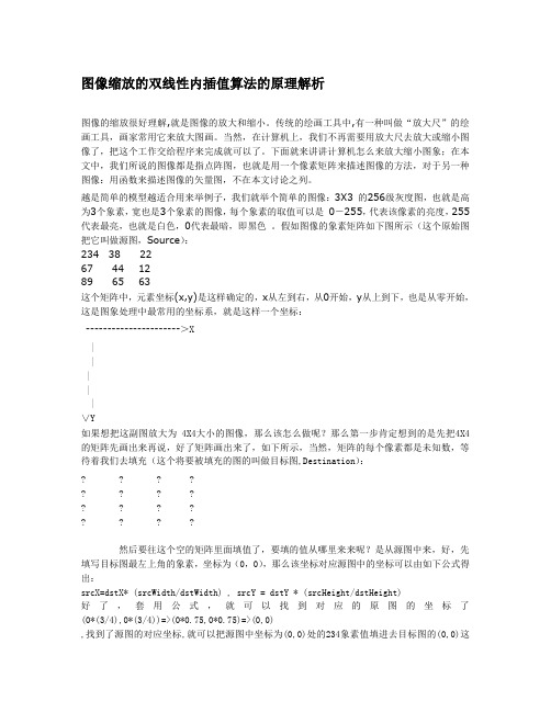
越是简单的模型越适合用来举例子,我们就举个简单的图像:3X3 的256级灰度图,也就是高为3个象素,宽也是3个象素的图像,每个象素的取值可以是0-255,代表该像素的亮度,255代表最亮,也就是白色,0代表最暗,即黑色。
假如图像的象素矩阵如下图所示(这个原始图把它叫做源图,Source):234 38 2267 44 1289 65 63这个矩阵中,元素坐标(x,y)是这样确定的,x从左到右,从0开始,y从上到下,也是从零开始,这是图象处理中最常用的坐标系,就是这样一个坐标:---------------------->X|||||∨Y如果想把这副图放大为 4X4大小的图像,那么该怎么做呢?那么第一步肯定想到的是先把4X4的矩阵先画出来再说,好了矩阵画出来了,如下所示,当然,矩阵的每个像素都是未知数,等待着我们去填充(这个将要被填充的图的叫做目标图,Destination):? ? ? ?? ? ? ?? ? ? ?? ? ? ?然后要往这个空的矩阵里面填值了,要填的值从哪里来来呢?是从源图中来,好,先填写目标图最左上角的象素,坐标为(0,0),那么该坐标对应源图中的坐标可以由如下公式得出:srcX=dstX* (srcWidth/dstWidth) , srcY = dstY * (srcHeight/dstHeight)好了,套用公式,就可以找到对应的原图的坐标了(0*(3/4),0*(3/4))=>(0*0.75,0*0.75)=>(0,0),找到了源图的对应坐标,就可以把源图中坐标为(0,0)处的234象素值填进去目标图的(0,0)这个位置了。
一种基于映射图像子块的图像缩小加权平均算法
一种基于映射图像子块的图像缩小加权平均算法
高健;茅时群;周宇玫;叶静
【期刊名称】《中国图象图形学报》
【年(卷),期】2006(011)010
【摘要】针对一般缩小算法随着缩小比例降低,图像信息丢失愈发严重的现象,提出了一种基于映射图像子块的图像缩小加权平均算法.首先,根据缩小比例,求出缩小图像中每点映射在原始图像中的子块,然后,根据各子块,加权平均算出缩小图像中每点的像素值,从而达到缩小的目的.缩小后的图像具有较好的完整性,且算法简单、快速有效.实验结果表明,该算法与其他缩小算法相比,在保持图像完整性方面具一定的特点.最后,针对缩小后图像对比度偏低这一现象,提出了一种灰度拉伸的处理方法,并进行了实验对比,取得了较好效果.
【总页数】4页(P1460-1463)
【作者】高健;茅时群;周宇玫;叶静
【作者单位】上海大学-纽帝亚联合媒体研究中心,上海,200072;上海大学-纽帝亚联合媒体研究中心,上海,200072;上海大学-纽帝亚联合媒体研究中心,上海,200072;上海大学-纽帝亚联合媒体研究中心,上海,200072
【正文语种】中文
【中图分类】TP391.4
【相关文献】
1.一种基于小波系数加权平均的Retinex图像增强算法 [J], 薛培;薛国新;张亚洲;刘强
2.一种基于小波系数加权平均的Retinex图像增强算法 [J], 薛培;薛国新;张亚洲;刘强
3.基于图像子块加权缩小的自适应修正算法 [J], 常军;吴锡生
4.一种基于角点信息和加权子块的图像缩小算法 [J], 徐御
5.基于多特征盒计数图像子块的道路图像的缩小 [J], 刘晟
因版权原因,仅展示原文概要,查看原文内容请购买。
图像缩放算法中常见插值方法比较
图像缩放算法中常见插值方法比较
陈高琳
【期刊名称】《福建电脑》
【年(卷),期】2017(033)009
【摘要】本文综合介绍了图像缩放算法中常用的几种插值方法,并对几种算法的基本原理和优缺点进行描述.最后通过实际的原始图像使用不同的图像缩放差值算法得到的输出结果,对比并阐述其不同的效果.
【总页数】2页(P98-99)
【作者】陈高琳
【作者单位】福建师范大学数学与信息学院福建福州 350007
【正文语种】中文
【相关文献】
1.聚束SAR成像算法中的几种插值方法比较 [J], 曾海彬;曾涛;胡程;朱宇
2.比较阅读中常见的比较点--从2005年中考文言文阅读题说起 [J], 张翼
3.基于R-D算法的合成孔径声纳插值方法比较 [J], 丁迎迎;孙超
4.实现图像缩放功能的Matlab插值算法研究与比较 [J], 丁雪晶
5.三种常见插值方法思想比较及适应性分析 [J], 于秀君
因版权原因,仅展示原文概要,查看原文内容请购买。
图像压缩算法的性能比较与分析
图像压缩算法的性能比较与分析一、引言图像是数字媒体中的重要形式之一。
图像文件通常非常大,当它们用于互联网、移动设备和存储时,大尺寸的图像会带来许多问题,例如占用太多的存储空间、传输速度缓慢、带宽限制等。
为了解决这些问题,图像压缩技术被广泛应用。
目前,常用的图像压缩算法有无损压缩和有损压缩两种类型。
它们在不同情况下有着相应的应用。
本文将介绍图像压缩的基本概念和不同算法的性能比较与分析。
二、基本概念2.1 无损压缩无损压缩是指对图像进行压缩,在压缩后的文件进行解压缩还原的图像与原始图像之间没有任何差异的压缩方法。
这种压缩方法是分析原始图像的重复模式,并学会使用更简单的指令表示这些模式。
无损压缩通常不会去掉图像本身中的任何信息,只是减小了文件的大小。
2.2 有损压缩有损压缩是指对图像进行压缩,在压缩后的文件进行解压缩还原的图像与原始图像之间有些许差异的压缩方法,这种差异可以通过人的肉眼来识别。
有损压缩方法通常通过去掉不重要的图像信息来减小文件大小。
2.3 像素在数字图像中,图像被分成很多缩小的单元格,这些单元格被称为像素。
每个像素包含有颜色和亮度信息。
2.4 分辨率在数字图像中,分辨率是指图像所包含的像素数量。
通常来说,分辨率越高,图像就越清晰。
三、图像压缩算法3.1 LZW算法LZW算法是最常用的无损压缩算法之一。
它基于一种字典,包含了所有可用的数据。
在使用LZW算法压缩图像时,其将存储在图像中的像素数据序列替换为相应的压缩代码。
如果LZW算法的压缩率足够高,则它可以有效地减少图像的大小。
3.2 JPEG算法JPEG是一种有损压缩算法。
它是基于离散余弦变换的,也被称为DCT算法。
JPEG算法通过分离图像中不同区域的颜色和亮度信息来减少文件大小。
在JPEG算法中,亮度信息被整合为一种通道(Y通道),而颜色信息被分离成另外两种通道(U和V通道)。
JPEG算法可以根据压缩比例的要求进行优化。
3.3 PNG算法PNG是Portable Network Graphics的缩写,是一种无损压缩算法。
几种最新的图像缩放方法的比较性研究的开题报告
几种最新的图像缩放方法的比较性研究的开题报告提纲:1.研究背景:图像缩放的应用和重要性2.研究问题:现有的图像缩放方法的不足和需要改进之处3.研究目的:评估几种最新的图像缩放方法的性能差异和适用性4.研究方法:实验评估和比较、数据分析和可视化5.预期结果:几种最新的图像缩放方法的性能差异和适用性6.研究意义:为图像缩放领域的技术发展提供参考和帮助优化图像处理和媒体应用。
正文:1.研究背景:图像缩放在计算机视觉和图像处理方面得到了广泛的应用,例如数字媒体和数字化文化遗产,身份验证、医学诊断和多媒体通信等领域。
图像缩放允许将图像的尺寸调整为不同的应用要求。
尽管存在多种方法可以实现图像缩放,但最新的图像缩放技术旨在提高缩放输出图像质量并减少图像失真。
2.研究问题虽然有许多图像缩放方法可供选择,但每种方法都有其优缺点。
例如,传统的双线性和双三次插值方法可能会导致图像加权平均和图像失真。
为了克服这些缺陷,研究人员提出了许多新的图像缩放方法,如超分辨率、深度卷积、反卷积网络、GAN等。
这种方法利用大量的训练数据,采用复杂模型,旨在更好地处理高分辨率图像。
但是,这些新方法是否在性能和适用性方面比传统的图像缩放方法更好,例如Bicubic缩放,目前尚未完全确定。
本研究旨在评估和比较几种最新的图像缩放方法(如超分辨率、深度卷积、反卷积网络和GAN等),并确定它们在图像缩放方面的性能和适用性。
首先,十几种方法将分为不同的组,并对其进行准确的实验评估和比较。
然后,将收集、分析和可视化结果数据,以确定每种方法的影响和优势。
4. 研究方法(1)收集数据集和图像样本选择公开的数据集或自定几个不同类型的、不同分辨率的图像样本进行实验,并比较为同一大小的输出图像。
(2)实验评估和比较根据前面阐述的几种方法,将数据集或图片样本分成不同的实验组,提供相应的参数和设置详细的实验环境,比较结果的不同(3)数据分析和可视化收集和比较各种方法的数据,对结果进行可视化或绘制图形,并分析所得数据,寻找差异或趋势。
- 1、下载文档前请自行甄别文档内容的完整性,平台不提供额外的编辑、内容补充、找答案等附加服务。
- 2、"仅部分预览"的文档,不可在线预览部分如存在完整性等问题,可反馈申请退款(可完整预览的文档不适用该条件!)。
- 3、如文档侵犯您的权益,请联系客服反馈,我们会尽快为您处理(人工客服工作时间:9:00-18:30)。
I.J. Image, Graphics and Signal Processing, 2013, 5, 55-62Published Online April 2013 in MECS (/)DOI: 10.5815/ijigsp.2013.05.07A Comparative Analysis of Image ScalingAlgorithmsChetan SureshDepartment of Electrical and Electronics Engineering, BITS PilaniPilani - 333031, Rajasthan, IndiaE-mail: shivchetan@Sanjay Singh, Ravi Saini, Anil K SainiScientist, IC Design Group,CSIR – Central Electronics Engineering Research Institute (CSIR-CEERI)Pilani – 333031, Rajasthan, IndiaAbstract—Image scaling, fundamental task of numerous image processing and computer vision applications, is the process of resizing an image by pixel interpolation. Image scaling leads to a number of undesirable image artifacts such as aliasing, blurring and moiré. However, with an increase in the number of pixels considered for interpolation, the image quality improves. This poses a quality-time trade off in which high quality output must often be compromised in the interest of computation complexity. This paper presents a comprehensive study and comparison of different image scaling algorithms. The performance of the scaling algorithms has been reviewed on the basis of number of computations involved and image quality. The search table modification to the bicubic image scaling algorithm greatly reduces the computational load by avoiding massive cubic and floating point operations without significantly losing image quality.Index Terms—Image Scaling, Nearest-neighbour, Bilinear, Bicubic, Lanczos, Modified BicubicI.I NTRODUCTIONImage scaling is a geometric transformation used to resize digital images and finds widespread use in computer graphics, medical image processing, military surveillance, and quality control [1]. It plays a key role in many applications [2] including pyramid construction [3]-[4], super-sampling, multi-grid solutions [5], and geometric normalization [6].In surveillance-based applications, images have to be monitored at a high frame rate. Since, the images need not be of the same size, image scaling is necessary for comparison and manipulation of images. However, image scaling is a computationally intensive process due to the convolution operation, which is necessary to band-limit the discrete input and thereby diminishes undesirable aliasing artifacts [2].Various image scaling algorithms are available in literature and employ different interpolation techniques to the same input image. Some of the common interpolation algorithms are the nearest neighbour, bilinear [7], and bicubic [8]-[9]. Lanczos algorithm utilizes the 3-lobed Lanczos window function to implement interpolation [10].There are many other higher order interpolators which take more surrounding pixels into consideration, and thus also require more computations. These algorithms include spline [11] and sinc interpolation [12], and retain the most of image details after an interpolation. They are extremely useful when the image requires multiple rotations/distortions in separate steps. However, for single-step enlargements or rotations, these higher-order algorithms provide diminishing visual improvement and processing time increases significantly.Novel interpolation algorithms have also been proposed such as auto-regression based method [13], fuzzy area-based scaling [14], interpolation using classification and stitching [15], isophote-based interpolation [16], and even interpolation scheme combined with Artificial Neural Networks [17]. Although these algorithms perform well, they require a lengthy processing time due to their complexity. This is intolerable for real-time image scaling in video surveillance system. Hence, these algorithms have not been considered for the comparative analysis in this paper.In this paper, firstly, image interpolation algorithms are classified and reviewed; then evaluation and comparison of five image interpolation algorithms are discussed in depth based on the reason that evaluation of image interpolation is essential in the aspect of designing a real-time video surveillance system. Analysis results of the five interpolation algorithms are summarized and presented.II.I MAGE S CALINGImage scaling is obtained by performing interpolation over one or two directions to approximate a pixel’s colour and intensity based on the values at neighbouringpixels. More the adjacent pixels used for interpolation, better the quality of interpolated output image. Digital image interpolation is the process of generating a continuous intensity surface from discrete image data samples. Generally, almost every geometric transformation like translating, rotating, scaling, and warping requires interpolation to be performed on an image [18]. Such transformations are essential to any commercial digital image processing software. The perceived quality of the interpolated images is affected by several issues such as sharpness of edges, freedom from artifacts and reconstruction of high frequency details [18].Interpolation algorithms attempt to generate continuous data from a set of discrete data samples through an interpolation function. These interpolation methods aim to minimize the visual defects arising from the inevitable resampling error and improve the quality of re-sampled images [19]. Interpolation function is performed by convolution operation which involves a large number of addition and multiplication operations. Hence, a trade-off is required between computation complexity and quality of the scaled image.Based on the content awareness of the algorithm, image scaling algorithms can be classified as Adaptive image scaling and Non-adaptive image scaling. Adaptive image scaling algorithms modify their interpolation technique based on the image content being a smooth texture [20] or a sharp edge [21]-[22]. As the interpolation method changes in real-time, these algorithms are complex and computationally intensive. They find widespread use in image editing software as they ensure a high quality scaled image. As the focus is on analysing image scaling algorithms for real-time applications, these algorithms are beyond the scope of the paper.Non-adaptive image scaling algorithms like nearest neighbour, bilinear, bicubic and Lanczos algorithms have a fixed interpolation method irrespective of the image content.III. C OMPARATIVE A NALYSIS OF I MAGE S CALINGA LGORITHMS This section discusses the Non-adaptive Image scaling algorithms like nearest neighbour, bilinear, bicubic, modified bicubic, and Lanczos. Let P(x,y) represent the pixel in input image of MxN dimensions and U(i,j) represents the pixel in scaled/resized output image of size M’xN’. Let T be the transformation used for scaling. The each pixel of output image is computed by applying the transformation T on input image pixels as shown inFig. 1.Figure 1. Image scaling procedureA. N EAREST N EIGHBOUR I MAGE S CALINGThe simplest image interpolation method is to select the value of the nearest input image pixel and assigning the same value to scaled image pixel. The nearest neighbour algorithm (Fig. 2) selects the value of the nearest known pixel and does not consider the values of other neighbouring pixels, yielding a piecewise constant function [23].For nearest neighbour algorithm the level of complexity is low leading to a fast computation time. But the scaled image quality is low and high aliasingeffect is observed.Figure 2. Nearest neighbour image scaling algorithmB. B ILINEAR I MAGE S CALINGAnother simple interpolation method is linear interpolation, a slight improvement over the nearest neighbour interpolation algorithm. In linear interpolation, the interpolated value is computed based on the weighted average of two data points. The weights are inversely proportional to the distance of the end points from the interpolated data point.Bilinear interpolation algorithm [7] performs linear interpolation in one direction followed by linear interpolation of the interpolated values in the other direction. The algorithm uses 4 diagonal pixels surrounding the corresponding source image pixel for interpolation (Fig. 3). It computes a weighted average depending on the nearness and brightness of the 4 diagonal pixels and assigns that value to the pixel in the output image.Figure 3. Bilinear image scaling algorithmBilinear offers considerable improvement in image quality with a slightly increased complexity. The aliasing effect is reduced though blurring is observed. C. B ICUBIC I MAGE S CALINGBicubic interpolation algorithm [8]-[9] performs cubic interpolation in one direction followed by cubic interpolation of the interpolated values in the otherdirection (Fig. 4).Figure 4. Bicubic image scaling algorithmThe bicubic interpolation approximates a sinc interpolation by using cubic polynomial waveforms instead of linear waveforms when computing an output pixel value. The algorithm uses 16 nearest pixelssurrounding the closest corresponding pixel in the source image for interpolation.Bicubic offers high scaled image quality at the cost of considerably high complexity. Edge halo effect is observed though aliasing and blurring are reduced. D. L ANCZOS I MAGE S CALINGThe Lanczos interpolation algorithm [10] uses a windowed form of sinc filter (an ideal low-pass filter) to perform interpolation on a 2-D grid. Sinc function of a variable can be mathematically obtained by dividing the sine function of the variable by itself [9]. Sinc function theoretically never goes to zero. Hence, a practical filter can be implemented by multiplying the sinc function with a window operator such as Hamming [24]-[25] and Hann [26] to obtain a filter with a finite size.The Lanczos filter can be obtained by multiplying the sinc function with the Lanczos window which is truncated to zero outside of the main lobe [27]. The size of the Lanczos window is defined by the order of theconvolution kernel.Figure 5. Lanczos image scaling algorithmThe number of neighbouring pixels considered varies as the order of the kernel. If the order is chosen to be 2, 16 pixels are considered while if the order is 3, 36 neighbouring pixels are utilized for interpolation. Forsufficient image quality, the order is chosen to be 3 in the implementation (Fig. 5).The Lanczos algorithm gives an output scaled image of the same quality as bicubic but at the cost of higher number of computations as 36 pixels is used for interpolating the value of each output pixel compared to 16 for bicubic. The Lanczos algorithm is comparatively more efficient for multiple scaling operations. E. M ODIFIED B ICUBIC I MAGE S CALINGAccording to the bicubic convolution kernel equation, massive calculations of four spots bicubic interpolation algorithm include large cubic and floating point multiplication operation. The bicubic interpolation algorithm discussed above can be slightly modified as shown below (Fig. 6). The co-efficients a0, a1, a2, a3, b0, b1, b2, and b3 are now a function of dx and dy (the difference between the interpolated co-ordinate and nearest integer source co-ordinate lower than it) instead of the interpolating pixels. This allows us to compute and store the values of the co-efficients for pre-determined values of dx and dy . This avoids the large number of cubic and floating point operations involved in bicubic interpolation.dy/6;*dy *dy + dy/6- = b3dy/2;*dy *dy - dy/2*dy +dy = b2dy/2;*dy *dy + dy/2*dy - dy/2 - 1 = b1dy/6;*dy *dy - /2dy *dy + /3dy - = b0dx/6;*dx *dx + dx/6- = a3dx/2;*dx *dx - dx/2*dx + dx = a2dx/2;*dx *dx + dx/2*dx - dx/2 - 1 = a1dx/6;*dx *dx - /2 dx * dx + /3 dx - = a0Where,C[3]*b3+C[2] *b2+C[1]*b1+C[0]*b0 = Cc d3*a3+ d2*a2+ d1*a1+d0*a0 =C[jj]Although the algorithm result has been influenced slightly, computation load is largely simplified. It mainly overcomes the disadvantage that hardware implementation of the algorithm is difficult due to many floating point computations.The search table modification to the bicubic interpolation algorithm is discussed in [28]. The distance, which the image regards as the unit length l, between two neighbouring pixels in the source image is divided equally into 16 sub-intervals. They are [0,1/16), [1/16,2/16), [2/16,3/16), [3/16,4/16), [4/16,5/16), [5/16,6/16), [6/16,7/16), [7/16,8/16), [8/16,9/16), [9/16,10/16), [10/16,11/16), [11/16,12/16), [12/16,13/16), [13/16,14/16), [14/16,15/16) and [15/16,1). The co-efficients for all 16 values of dx and dy can be computed beforehand and stored in memory. This reduces the computationally intensive process of determining the co-efficients in real-time. The value of dx and dy is compared to lie within one of the 16 sub-intervals and the values of coefficients a0, a1, a2, a2, b1,b2, b3, and b4 are chosen accordingly from pre-computed values.Figure 6. Modified bicubic image scaling algorithmIV. RESULT ANALYSISAll five algorithms are implemented in C/C++ language. OpenCV libraries are used for image read and write/display only. Dev-C++ (4.9.9.2) software installed on a standard Window XP machine is used for compilation and execution of C/C++ programs. Comparison of computational complexity of all five image scaling algorithms is shown in Table 1. Input test image of size 627x462 and corresponding scaled output images of size 150x150 produced by five implementations are shown in Fig. 7. Fig. 8 shows the input test image of size 609x594 and corresponding scaled output images of size 150x150 produced by five implementations.Non-adaptive algorithms always face a trade-off between the three image scaling artifacts – edge halo, blurring and aliasing. Nearest neighbour interpolation produces a high aliasing effect resulting in jagged edges. Bilinear interpolation reduces the aliasing effect but causes a moderate blurring of the edges. Bicubic interpolation produces a moderate aliasing, blurring and an edge halo effect. Lanczos interpolation delivers an image quality very similar to that of bicubic. Modified bicubic produces an output of slightly lesser quality as compared to bicubic as the co-efficients are approximated to reduce computational complexity. Computationally, nearest neighbour interpolation is the least intensive as it considers only one pixel forinterpolation. Bilinear uses 4 diagonal pixels for interpolation and therefore, requires more computation than the nearest neighbour method. Bicubic and Lanczos interpolation are computationally very intensive as they require 16 and 36 pixels respectively for interpolating an output pixel value. Lanczos interpolation also utilizes the sine function repeatedly which itself requires a large number of addition and multiplication operations according to Taylor series approximation. Modified bicubic interpolation reduces the number of computations significantly as the co-efficients are computed using search table.Table 1 : Computational Complexity ComparisonFigure 7. Input test image and corresponding output image for each algorithmFigure 8. Input test image and corresponding output image for each algorithmV.C ONCLUSIONImage scaling has become a fundamental processing task and plays an important role in video surveillance applications. Although there are a myriad of interpolation algorithms are available in literature, not all of them are suitable for implementing real-time image scaling. In this paper, we discussed the main non-adaptive image interpolation algorithms suitable for real-time applications. A comparative analysis of five image interpolation algorithms is presented based on the results of their software implementation. Of the five image interpolation algorithms evaluated, the modified bicubic algorithm offers the best trade-off between image quality and computational complexity for real-time image scaling in surveillance applications.A CKNOWLEDGMENTThe authors express their deep sense of gratitude to Dr. Chandra Shekhar, Director CSIR-CEERI for encouraging research and development activities. Authors would like to thanks Dr. AS Mandal and Raj Singh, Group Leader, IC Design Group, CSIR-CEERI, for their constructive suggestions throughout the year.R EFERENCES[1]J. Xiao, X. Zou, Z. Liu, X. Gu, A Novel AdaptiveInterpolation Algorithm For Image Resizing, International Journal of Innovative Computing,Information and Control, Vol. 3, n. 6(A), pp. 1335-1345, 2007.[2]Wolberg, G., Massalin, H., A Fast Algorithm forDigital Image Scaling, Proceedings of Computer Graphics International (Year of Publication: 1993).[3] F. Chin, A. Choi, Y. Luo, Optimal GeneratingKernels for Image Pyramids by Piecewise Fitting, IEEE Transactions on Pattern Analysis and Machine Intelligence, Vol. 14, n. 12, pp. 1190-1198, 1992.[4]P. Meer, E.S. Baugher, A. Rosenfeld, FrequencyDomain Analysis and Synthesis of Image Pyramid Generating Kernels, IEEE Transactions on Pattern Analysis and Machine Intelligence, Vol. PAMI-9, n.4, pp. 512-522, 1987.[5]P.P.Vaidyanathan, Multirate Systems and FilterBanks (Prentice Hall, 1993).[6]G. Wolberg, Digital Image Warping(IEEEComputer Society Press, 1992).[7]W.H. Press, B.P. Flannery, S.A. Teukolsky, W.T.Vetterling, Numerical Recipes: The Art of Scientific Computing (FORTRAN Version) (Cambridge University Press, 1989).[8] C. Boor, A Practical Guide to Splines (Springer-Verlag, 1978).[9]R.C. Gonzalez, R.E. Woods, Digital ImageProcessing (Prentice Hall, 2007).[10]K. Turkowski, Filters for common resampling tasks,In A.S. Glassner (Ed.), Graphic Gems, 4(San Diego: Academic Press, 1990, 147-170).[11]M. Unser, A. Aldroubi, M. Eden, Fast B-SplineTransforms for Continuous Image Representation and Interpolation, IEEE Transactions on Pattern Analysis and Machine Intelligence, Vol. 13, n. 3, pp.277-285, 1991.[12]Meijering, E.H.W., Niessen, W.J., Viergever, M.A.,The sinc-approximating kernels of classical polynomial interpolation, Proceedings of the International Conference on Image Processing (Page: 652-656 Year of Publication: 1999 ISBN:0-7803-5467-2).[13]Zhe, W., Jiefu, Z., Mengchu, Z., A FastAutoregression Based Image Interpolation Method, Proceedings of the IEEE International Conference on Networking, Sensing and Control (Page: 1400-1404 Year of Publication: 2008 ISBN:978-1-4244-1685-1).[14]Amanatiadis, A., Andreadis, I., Konstatinidis, K.,Fuzzy Area-Based Image Scaling, Proceedings of the IEEE Instrumentation and Measurement Technology Conference (Page: 1-6 Year of Publication: 2007 ISBN:1-4244-0588-2).[15]Mueller, N., Nguyen, T.K., Image interpolationusing classification and stitching, Proceedings of the IEEE International Conference on Image Processing (Page: 901-904 Year of Publication: 2008 ISBN:978-1-4244-1765-0).[16]Morse, B.S., Schwartzwald, D., Isophote-basedinterpolation, Proceedings of the IEEE International Conference on Image Processing (Page: 227-231 Year of Publication: 1998 ISBN:0-8186-8821-1). [17]Liang, F., Xie, K., An Image Interpolation Schemecombined with Artificial Neural Network, Proceedings of the Third International Conference on Natural Computation (Page: 99-102 Year of Publication: 2007 ISBN:978-0-7695-2875-5). [18]S.D. Ruikar, D.D. Doye, Image Denoising using TriNonlinear and Nearest Neighbour Interpolation with Wavelet Transform, International Journal of Information Technology and Computer Science, Vol.4, n. 9, pp. 36-44, 2012.[19]D. Su, P. Willis, Image Interpolation by Pixel LevelData-Dependent Triangulation,Computer Graphics Forum, Vol.23, n. 2, pp. 189-201, 2004.[20]Zhang, J., Kuo, C., Region-adaptive Texture-awareImage Resizing, Proceedings of the IEEE International Conference on Acoustics, Speech and Signal Processing (Page: 837-840 Year of Publication: 2012 ISBN:978-1-4673-0045-2). [21]Jiang, W., Xu, H., Chen, G., Zhao, W., Xu, W., AnImproved Edge-adaptive Image Scaling Algorithm, Proceedings of the IEEE Eighth InternationalConference on ASIC (Page: 895-897 Year of Publication: 2009 ISBN:978-1-4244-3868-6). [22]Lai, Y., Tzeng, C., Wu, H., Adaptive Image ScalingBased on Local Edge Directions, Proceedings of the International Conference on Intelligent and Advanced Systems (Page: 1-4 Year of Publication: 2010 ISBN:978-1-4244-6623-8).[23]Jenkins, W., Mather, B., Munson, D., Jr., NearestNeighbor And Generalized Inverse Distance Interpolation For Fourier Domain Image Reconstruction, Proceedings of the IEEE International Conference on Acoustics, Speech and Signal Processing (Page: 1069-1072 Year of Publication: 1985).[24]W. Ye, A. Entezari, A Geometric Construction ofMultivariate Sinc Functions, IEEE Transactions on Image Processing, Vol.21, n. 6, pp. 2969-2979, 2012.[25]Xiao, L., Dong, X., Soong, A.C.K., EffectiveInterpolator Design for Pilot Symbol Assisted Modulation Systems, Proceedings of the IEEE Global Telecommunications Conference (Page: 3671-3675 Year of Publication: 2004 ISBN:0-7803-8794-5).[26]Wenbo, T., Jianming, Y., Xiaojin, M., Ji, L., Powersystem harmonic detection based on Bartlett–Hann Windowed FFT interpolation, Proceedings of the Asia-Pacific Power and Energy Engineering Conference (Page: 1-3 Year of Publication: 2012 ISBN:978-1-4577-0545-8).[27]Ye, Z., Suri, J., Sun, Y., Janer, R., Four ImageInterpolation Techniques for Ultrasound Breast Phantom Data Acquired Using Fischer's Full Field Digital Mammography and Ultrasound System (FFDMUS): A Comparative Approach, Proceedings of the IEEE International Conference on Image Processing (Page: 1238-1241 Year of Publication: 2005 ISBN:0-7803-9134-9).[28]Zhang, Y., Li, Y., Zhen, J., The HardwareRealization of Bicubic Interpolation Enlargement Algorithm Based on FPGA, Proceedings of the Third International Symposium on Information Processing (Page: 277-281 Year of Publication: 2010 ISBN:978-1-4244-8627-4).Chetan Suresh is pursuing hisundergraduate study in BITS-Pilani,Rajasthan, India. He is a final yearstudent of Electrical and ElectronicsEngineering. Currently, he isworking as a student intern inCambridge Silicon Radio, Bangalore. His research interests are FPGA Prototyping and Computer Architecture.Sanjay Singh is workingas Scientist in CSIR-CentralElectronics Engineering ResearchInstitute, Pilani, Rajasthan, India. Heis Member of IEEE - USA, IACSIT- Singapore, and IAENG - HongKong. Currently, he is involved in various projects sponsored by Indian Government on Computer Vision and Smart Cameras. His research interests are VLSI architectures for image & video processing algorithms, FPGA Prototyping, and Computer Vision. Prior to joining this research lab, he received his Master in Technology, Master in Electronics, and Bachelor in Science in 2007, 2005, and 2003 respectively from Kurukshetra University, Kurukshetra, Haryana, India. He earned Gold Medal (First Position in University) during his Master in Technology and Master in Electronics. He topped college during his Bachelor in Science. He received more than 20 Merit Certificates and Scholarships during his academic career.Ravi Saini is working as Scientist inCSIR-Central ElectronicsEngineering Research Institute,Pilani, Rajasthan, India. He isMember of IEEE –USA. Hisresearch interests include VLSIArchitectures, ASIC and ASIPDesign, HDLs, and FPGA Prototyping. He received his Master in Technology in 2002 from Punjab University, India and Master in Electronics in 2000 from DAVV, Indore, India.Anil Kumar Saini is workingas Scientist in CSIR-CentralElectronics Engineering ResearchInstitute, Pilani, Rajasthan, India.He is Member of IEEE – USA andIACSIT –Singapore. His researchinterests include Analog andMixed Signal Design, Embedded System Design, and CMOS RF IC design. Prior to joining this research lab, he worked in Cadence, India. He received his Master in Technology and Master in Science in 2003 and 2000 respectively from IIT Roorkee, India.。