实验排队论问题的编程实现
排队系统仿真matlab实验报告

M/M/1排队系统实验报告一、实验目的本次实验要求实现M/M/1单窗口无限排队系统的系统仿真,利用事件调度法实现离散事件系统仿真,并统计平均队列长度以及平均等待时间等值,以与理论分析结果进行对比。
二、实验原理根据排队论的知识我们知道,排队系统的分类是根据该系统中的顾客到达模式、服务模式、服务员数量以及服务规则等因素决定的。
1、 顾客到达模式设到达过程是一个参数为λ的Poisson 过程,则长度为t 的时间内到达k 个呼叫的概率 服从Poisson 分布,即e t kk k t t p λλ-=!)()(,⋅⋅⋅⋅⋅⋅⋅⋅⋅=,2,1,0k ,其中λ>0为一常数,表示了平均到达率或Poisson 呼叫流的强度。
2、 服务模式设每个呼叫的持续时间为i τ,服从参数为μ的负指数分布,即其分布函数为{}1,0t P X t e t μ-<=-≥3、 服务规则先进先服务的规则(FIFO )4、 理论分析结果在该M/M/1系统中,设λρμ=,则稳态时的平均等待队长为1Q ρλρ=-,顾客的平均等待时间为T ρμλ=-。
三、实验内容M/M/1排队系统:实现了当顾客到达分布服从负指数分布,系统服务时间也服从负指数分布,单服务台系统,单队排队,按FIFO (先入先出队列)方式服务。
四、采用的语言MatLab 语言源代码:clear;clc;%M/M/1排队系统仿真SimTotal=input('请输入仿真顾客总数SimTotal='); %仿真顾客总数;Lambda=0.4; %到达率Lambda;Mu=0.9; %服务率Mu;t_Arrive=zeros(1,SimTotal);t_Leave=zeros(1,SimTotal);ArriveNum=zeros(1,SimTotal);LeaveNum=zeros(1,SimTotal);Interval_Arrive=-log(rand(1,SimTotal))/Lambda;%到达时间间隔Interval_Serve=-log(rand(1,SimTotal))/Mu;%服务时间t_Arrive(1)=Interval_Arrive(1);%顾客到达时间ArriveNum(1)=1;for i=2:SimTotalt_Arrive(i)=t_Arrive(i-1)+Interval_Arrive(i);ArriveNum(i)=i;endt_Leave(1)=t_Arrive(1)+Interval_Serve(1);%顾客离开时间LeaveNum(1)=1;for i=2:SimTotalif t_Leave(i-1)<t_Arrive(i)t_Leave(i)=t_Arrive(i)+Interval_Serve(i);elset_Leave(i)=t_Leave(i-1)+Interval_Serve(i);endLeaveNum(i)=i;endt_Wait=t_Leave-t_Arrive; %各顾客在系统中的等待时间t_Wait_avg=mean(t_Wait);t_Queue=t_Wait-Interval_Serve;%各顾客在系统中的排队时间t_Queue_avg=mean(t_Queue);Timepoint=[t_Arrive,t_Leave];%系统中顾客数随时间的变化Timepoint=sort(Timepoint);ArriveFlag=zeros(size(Timepoint));%到达时间标志CusNum=zeros(size(Timepoint));temp=2;CusNum(1)=1;for i=2:length(Timepoint)if (temp<=length(t_Arrive))&&(Timepoint(i)==t_Arrive(temp)) CusNum(i)=CusNum(i-1)+1;temp=temp+1;ArriveFlag(i)=1;elseCusNum(i)=CusNum(i-1)-1;endend%系统中平均顾客数计算Time_interval=zeros(size(Timepoint));Time_interval(1)=t_Arrive(1);for i=2:length(Timepoint)Time_interval(i)=Timepoint(i)-Timepoint(i-1);endCusNum_fromStart=[0 CusNum];CusNum_avg=sum(CusNum_fromStart.*[Time_interval 0] )/Timepoint(end);QueLength=zeros(size(CusNum));for i=1:length(CusNum)if CusNum(i)>=2QueLength(i)=CusNum(i)-1;elseQueLength(i)=0;endendQueLength_avg=sum([0 QueLength].*[Time_interval 0] )/Timepoint(end);%系统平均等待队长%仿真图figure(1);set(1,'position',[0,0,1000,700]);subplot(2,2,1);title('各顾客到达时间和离去时间');stairs([0 ArriveNum],[0 t_Arrive],'b');hold on;stairs([0 LeaveNum],[0 t_Leave],'y');legend('到达时间','离去时间');hold off;subplot(2,2,2);stairs(Timepoint,CusNum,'b')title('系统等待队长分布');xlabel('时间');ylabel('队长');subplot(2,2,3);title('各顾客在系统中的排队时间和等待时间');stairs([0 ArriveNum],[0 t_Queue],'b');hold on;stairs([0 LeaveNum],[0 t_Wait],'y');hold off;legend('排队时间','等待时间');%仿真值与理论值比较disp(['理论平均等待时间t_Wait_avg=',num2str(1/(Mu-Lambda))]);disp(['理论平均排队时间t_Wait_avg=',num2str(Lambda/(Mu*(Mu-Lambda)))]);disp(['理论系统中平均顾客数=',num2str(Lambda/(Mu-Lambda))]);disp(['理论系统中平均等待队长=',num2str(Lambda*Lambda/(Mu*(Mu-Lambda)))]);disp(['仿真平均等待时间t_Wait_avg=',num2str(t_Wait_avg)])disp(['仿真平均排队时间t_Queue_avg=',num2str(t_Queue_avg)])disp(['仿真系统中平均顾客数=',num2str(CusNum_avg)]);disp(['仿真系统中平均等待队长=',num2str(QueLength_avg)]);五、数据结构1.仿真设计算法(主要函数)利用负指数分布与泊松过程的关系,产生符合泊松过程的顾客流,产生符合负指数分布的随机变量作为每个顾客的服务时间:Interval_Arrive=-log(rand(1,SimTotal))/Lambda;%到达时间间隔,结果与调用exprnd(1/Lambda,m)函数产生的结果相同Interval_Serve=-log(rand(1,SimTotal))/Mu;%服务时间间隔t_Arrive(1)=Interval_Arrive(1);%顾客到达时间时间计算t_Wait=t_Leave-t_Arrive;%各顾客在系统中的等待时间t_Queue=t_Wait-Interval_Serve; %各顾客在系统中的排队时间由事件来触发仿真时钟的不断推进。
排队模拟实验C++语言代码

void CMy1Dlg::OnOK(){// TODO: Add extra validation hereUpdateData(TRUE);if (m_num<1&&m_num>6){AfxMessageBox("请输入1到5的数字!");return;}int T=m_num;UpdateData(false);ofstream file;file.open("新建.txt",ios::out);if(!file){cout<<"新建.txt can't open"<<endl;abort();}int i=1,X=0,D=0,zj=0,xhcs=0;file<<" 排队过程的模拟表"<<endl;file<<"-----------------------------------------------------------"<<endl;file<<" 随机数"<<" 到达数"<<" 需要卸货车数"<<" 卸货车数"<<" 推迟卸货车数"<<endl;srand(GetTickCount());while(i!=1000){int ran=rand()%10000;file<<setw(6)<<ran;if (ran<2300)X=0;else if(ran>=2300&&ran<5300)X=1;else if(ran>=5300&&ran<8300)X=2;else if(ran>=8300&&ran<9300)X=3;else if(ran>=9300&&ran<9700)X=4;elseX=5;file<<setw(6)<<X;int R;//R为需要卸货,D为推迟卸货,X为到达R=X+D;file<<setw(12)<<R;if (R<=T){file<<setw(12)<<R;D=0;}else{file<<setw(12)<<T;D=R-T;}file<<setw(12)<<D<<endl;zj+=X;if(D!=0)xhcs+=1;i++;}file<<"总计:"<<zj<<" "<<xhcs<<endl;file.close();fstream ifile("新建.txt",ios::in);MessageBox("请看文件<新建.txt>查看结果!");CDialog::OnOK();}。
排队论问题实验报告(3篇)

第1篇一、实验背景排队论是运筹学的一个重要分支,主要研究在服务系统中顾客的等待时间和服务效率等问题。
在现实生活中,排队现象无处不在,如银行、医院、超市、餐厅等。
通过对排队问题的研究,可以帮助我们优化服务系统,提高顾客满意度,降低运营成本。
本实验旨在通过模拟排队系统,探究排队论在实际问题中的应用。
二、实验目的1. 理解排队论的基本概念和原理。
2. 掌握排队模型的建立方法。
3. 熟悉排队系统参数的估计和调整。
4. 分析排队系统的性能指标,如平均等待时间、服务效率等。
5. 培养运用排队论解决实际问题的能力。
三、实验内容1. 建立排队模型本实验以银行排队系统为例,建立M/M/1排队模型。
该模型假设顾客到达服从泊松分布,服务时间服从负指数分布,服务台数量为1。
2. 参数估计根据实际数据,估计排队系统参数。
假设顾客到达率为λ=2(人/分钟),服务时间为μ=5(分钟/人)。
3. 模拟排队系统使用计算机模拟排队系统,记录顾客到达、等待、服务、离开等过程。
4. 性能分析分析排队系统的性能指标,如平均等待时间、服务效率、顾客满意度等。
四、实验步骤1. 初始化参数设置顾客到达率λ、服务时间μ、服务台数量n。
2. 生成顾客到达序列根据泊松分布生成顾客到达序列。
3. 模拟排队过程(1)当服务台空闲时,允许顾客进入队列。
(2)当顾客进入队列后,开始计时,等待服务。
(3)当服务台服务完毕,顾客离开,开始下一个顾客的服务。
4. 统计性能指标记录顾客等待时间、服务时间、顾客满意度等数据。
5. 分析结果根据实验数据,分析排队系统的性能,并提出优化建议。
五、实验结果与分析1. 平均等待时间根据模拟结果,平均等待时间为2.5分钟。
2. 服务效率服务效率为80%,即每分钟处理0.8个顾客。
3. 顾客满意度根据模拟结果,顾客满意度为85%。
4. 优化建议(1)增加服务台数量,提高服务效率。
(2)优化顾客到达率,降低顾客等待时间。
(3)调整服务时间,缩短顾客等待时间。
排队论使用lingo编写
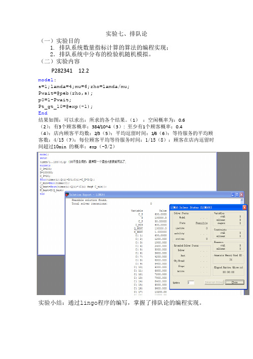
p0=1-Pwait;
Pt_gt_1可以求出:所求的各个结果。(1):空闲概率为:0.6
(2):有3个顾客概率:384/10^4(3):至少有1个顾客概率:0.4
(4):店内顾客平均数:2/3(5):平均逗留时间:1/6(6):等待服务的平均顾客数:4/15(7):每位顾客平均等待服务时间:1/15(8):顾客在店内逗留时间超过10min的概率:exp(-3/2)
实验七排队论一实验目的排队系统数量指标计算的算法的编程实现
实验七、排队论
(一)实验目的
1.排队系统数量指标计算的算法的编程实现;
2.排队系统中分布的检验机随机模拟。
(二)实验内容
P282341 12.2
model:
s=1;lamda=4;mu=6;rho=lamda/mu;
Pwait=@peb(rho,s);
queuing modeling排队论的matlab仿真(包括仿真代码)

Wireless Network Experiment Three: Queuing TheoryABSTRACTThis experiment is designed to learn the fundamentals of the queuing theory. Mainly about the M/M/S and M/M/n/n queuing MODELS.KEY WORDS: queuing theory, M/M/s, M/M/n/n, Erlang B, Erlang C. INTRODUCTIONA queue is a waiting line and queueing theory is the mathematical theory of waiting lines. More generally, queueing theory is concerned with the mathematical modeling and analysis of systems that provide service to random demands. In communication networks, queues are encountered everywhere. For example, the incoming data packets are randomly arrived and buffered, waiting for the router to deliver. Such situation is considered as a queue. A queueing model is an abstract description of such a system. Typically, a queueing model represents (1) the system's physical configuration, by specifying the number and arrangement of the servers, and (2) the stochastic nature of the demands, by specifying the variability in the arrival process and in the service process.The essence of queueing theory is that it takes into account the randomness of the arrival process and the randomness of the service process. The most common assumption about the arrival process is that the customer arrivals follow a Poisson process, where the times between arrivals are exponentially distributed. The probability of the exponential distribution function●Erlang B modelOne of the most important queueing models is the Erlang B model (i.e., M/M/n/n). It assumes that the arrivals follow a Poisson process and have a finite n servers. In Erlang B model, it assumes that the arrival customers are blocked and cleared when all the servers are busy. The blocked probability of a Erlang B model is given by the famous Erlang B formula,w here n is the number of servers and A= is the offered load in Erlangs, is the arrival rate and is the average service time. Formula (1.1) is hard to calculate directly from its right side when n and A are large. However, it is easy to calculate it using the following iterative scheme:●Erlang C modelThe Erlang delay model (M/M/n) is similar to Erlang B model, except that now it assumes that the arrival customers are waiting in a queue for a server to become available without considering the length of the queue. The probability of blocking (all the servers are busy) is given by the Erlang C formula,Where if and if . The quantity indicates the server utilization. The Erlang C formula (1.3) can be easily calculated by the following iterative schemewhere is defined in Eq.(1.1).DESCRIPTION OF THE EXPERIMENTSing the formula (1.2), calculate the blocking probability of the Erlang B model.Draw the relationship of the blocking probability PB(n,A) and offered traffic A with n = 1,2, 10, 20, 30, 40, 50, 60, 70, 80, 90, 100. Compare it with the table in the text book (P.281, table 10.3).From the introduction, we know that when the n and A are large, it is easy to calculate the blocking probability using the formula 1.2 as follows.it use the theory of recursion for the calculation. But the denominator and the numerator of the formula both need to recurs() when doing the matlab calculation, it waste time and reduce the matlab calculation efficient. So we change the formula to be :Then the calculation only need recurs once time and is more efficient.The matlab code for the formula is: erlang_b.m%**************************************% File: erlanb_b.m% A = offered traffic in Erlangs.% n = number of truncked channels.% Pb is the result blocking probability.%**************************************function [ Pb ] = erlang_b( A,n )if n==0Pb=1; % P(0,A)=1elsePb=1/(1+n/(A*erlang_b(A,n-1))); % use recursion "erlang(A,n-1)" endendAs we can see from the table on the text books, it uses the logarithm coordinate, so we also use the logarithm coordinate to plot the result. We divide the number of servers(n) into three parts, for each part we can define a interval of the traffic intensity(A) based on the figure on the text books :1. when 0<n<10, 0.1<A<10.2. when 10<n<20, 3<A<20.3. when 30<n<100, 13<A<120.For each part, use the “erlang_b”function to calculate and then use “loglog”function to figure the logarithm coordinate.The matlab code is :%*****************************************% for the three parts.% n is the number servers.% A is the traffic indensity.% P is the blocking probability.%*****************************************n_1 = [1:2];A_1 = linspace(0.1,10,50); % 50 points between 0.1 and 10.n_2 = [10:10:20];A_2 = linspace(3,20,50);n_3 = [30:10:100];A_3 = linspace(13,120,50);%*****************************************% for each part, call the erlang_b() function.%*****************************************for i = 1:length(n_1)for j = 1:length(A_1)p_1(j,i) = erlang_b(A_1(j),n_1(i));endendfor i = 1:length(n_2)for j = 1:length(A_2)p_2(j,i) = erlang_b(A_2(j),n_2(i));endendfor i = 1:length(n_3)for j = 1:length(A_3)p_3(j,i) = erlang_b(A_3(j),n_3(i));endend%*****************************************% use loglog to figure the result within logarithm coordinate. %*****************************************loglog(A_1,p_1,'k-',A_2,p_2,'k-',A_3,p_3,'k-');xlabel('Traffic indensity in Erlangs (A)')ylabel('Probability of Blocking (P)')axis([0.1 120 0.001 0.1])text(.115, .115,'n=1')text(.6, .115,'n=2')text(7, .115,'10')text(17, .115,'20')text(27, .115,'30')text(45, .115,'50')text(100, .115,'100')The figure on the text books is as follow:We can see from the two pictures that, they are exactly the same with each other except that the result of the experiment have not considered the situation with n=3,4,5,…,12,14,16,18.ing the formula (1.4), calculate the blocking probability of the Erlang C model.Draw the relationship of the blocking probability PC(n,A) and offered traffic A with n = 1,2, 10, 20, 30, 40, 50, 60, 70, 80, 90, 100.From the introduction, we know that the formula 1.4 is :Since each time we calculate the , we need to recurs n times, so the formula is not efficient. We change it to be:Then we only need recurs once. is calculated by the “erlang_b” function as step 1.The matlab code for the formula is : erlang_c.m%**************************************% File: erlanb_b.m% A = offered traffic in Erlangs.% n = number of truncked channels.% Pb is the result blocking probability.% erlang_b(A,n) is the function of step 1.%**************************************function [ Pc ] = erlang_c( A,n )Pc=1/((A/n)+(n-A)/(n*erlang_b(A,n)));endThen to figure out the table in the logarithm coordinate as what shown in the step 1.The matlab code is :%*****************************************% for the three parts.% n is the number servers.% A is the traffic indensity.% P_c is the blocking probability of erlangC model.%*****************************************n_1 = [1:2];A_1 = linspace(0.1,10,50); % 50 points between 0.1 and 10.n_2 = [10:10:20];A_2 = linspace(3,20,50);n_3 = [30:10:100];A_3 = linspace(13,120,50);%*****************************************% for each part, call the erlang_c() function.%*****************************************for i = 1:length(n_1)for j = 1:length(A_1)p_1_c(j,i) = erlang_c(A_1(j),n_1(i));%µ÷Óú¯Êýerlang_cendendfor i = 1:length(n_2)for j = 1:length(A_2)p_2_c(j,i) = erlang_c(A_2(j),n_2(i));endendfor i = 1:length(n_3)for j = 1:length(A_3)p_3_c(j,i) = erlang_c(A_3(j),n_3(i));endend%*****************************************% use loglog to figure the result within logarithm coordinate. %*****************************************loglog(A_1,p_1_c,'g*-',A_2,p_2_c,'g*-',A_3,p_3_c,'g*-');xlabel('Traffic indensity in Erlangs (A)')ylabel('Probability of Blocking (P)')axis([0.1 120 0.001 0.1])text(.115, .115,'n=1')text(.6, .115,'n=2')text(6, .115,'10')text(14, .115,'20')text(20, .115,'30')text(30, .115,'40')text(39, .115,'50')text(47, .115,'60')text(55, .115,'70')text(65, .115,'80')text(75, .115,'90')text(85, .115,'100')The result of blocking probability table of erlang C model.Then we put the table of erlang B and erlang C in the one figure, to compare their characteristic.The line with ‘ * ’ is the erlang C model, the line without ‘ * ’ is the erlang B model. We can see from the picture that, for a constant traffic intensity (A), the erlang C model has a higher blocking probability than erlang B model. The blocking probability is increasing with traffic intensity. The system performs better when has a larger n.ADDITIONAL BONUSWrite a program to simulate a M/M/k queue system with input parameters of lamda, mu, k.In this part, we will firstly simulate the M/M/k queue system use matlab to get the figure of the performance of the system such as the leave time of each customer and the queue lengthof the system.About the simulation, we firstly calculate the arrive time and the leave time for each customer. Then analysis out the queue length and the wait time for each customer use “for” loops.Then we let the input to be lamda = 3, mu = 1 and S = 3, and analysis performance of the system for the first 10 customers in detail.Finally, we will do two test to compared the performance of the system with input lamda = 1, mu = 1 and S = 3 and the input lamda = 4, mu = 1 and S = 3.The matlab code is:mms_function.mfunction[block_rate,use_rate]=MMS_function(mean_arr,mean_serv,peo_num,server_num) %%%%%%%%%%%%%%%%%%%%%%%%%%%%%%%%%%%%%%%%%%%%% %%%%%%%%%%%%%%%%%%%%%%%%%%%%first part: compute the arriving time interval, service time%interval,waiting time, leaving time during the whole service interval %%%%%%%%%%%%%%%%%%%%%%%%%%%%%%%%%%%%%%%%%%%%% %%%%%%%%%%%%%%%%%%%%%%%%%%%state=zeros(5,peo_num);%represent the state of each customer by%using a 5*peo_num matrix%the meaning of each line is: arriving time interval, service time%interval, waiting time, queue length when NO.ncustomer%arrive, leaving timestate(1,:)=exprnd(1/mean_arr,1,peo_num);%arriving time interval between each%customer follows exponetial distributionstate(2,:)=exprnd(1/mean_serv,1,peo_num);%service time of each customer follows exponetial distributionfor i=1:server_numstate(3,1:server_num)=0;endarr_time=cumsum(state(1,:));%accumulate arriving time interval to compute%arriving time of each customerstate(1,:)=arr_time;state(5,1:server_num)=sum(state(:,1:server_num));%compute living time of first NO.server_num%customer by using fomular arriving time + service timeserv_desk=state(5,1:server_num);%create a vector to store leaving time of customers which is in service for i=(server_num+1):peo_numif arr_time(i)>min(serv_desk)state(3,i)=0;elsestate(3,i)=min(serv_desk)-arr_time(i);%when customer NO.i arrives and the%server is all busy, the waiting time can be compute by%minus arriving time from the minimum leaving timeendstate(5,i)=sum(state(:,i));for j=1:server_numif serv_desk(j)==min(serv_desk)serv_desk(j)=state(5,i);breakend%replace the minimum leaving time by the first waiting customer'sleaving timeendend%%%%%%%%%%%%%%%%%%%%%%%%%%%%%%%%%%%%%%%%%%%%% %%%%%%%%%%%%%%%%%%%%%%%%%%%%second part: compute the queue length during the whole service interval %%%%%%%%%%%%%%%%%%%%%%%%%%%%%%%%%%%%%%%%%%%%% %%%%%%%%%%%%%%%%%%%%%%%%%%zero_time=0;%zero_time is used to identify which server is emptyserv_desk(1:server_num)=zero_time;block_num=0;block_line=0;for i=1:peo_numif block_line==0find_max=0;for j=1:server_numif serv_desk(j)==zero_timefind_max=1; %means there is empty serverbreakelse continueendendif find_max==1%update serv_deskserv_desk(j)=state(5,i);for k=1:server_numif serv_desk(k)<arr_time(i) %before the NO.i customer actually arrivesthere maybe some customerleaveserv_desk(k)=zero_time;else continueendendelseif arr_time(i)>min(serv_desk)%if a customer will leave before the NO.i%customer arrivefor k=1:server_numif arr_time(i)>serv_desk(k)serv_desk(k)=state(5,i);breakelse continueendendfor k=1:server_numif arr_time(i)>serv_desk(k)serv_desk(k)=zero_time;else continueendendelse %if no customer leave before the NO.i customer arriveblock_num=block_num+1;block_line=block_line+1;endendelse %the situation that the queue length is not zeron=0;%compute the number of leaing customer before the NO.i customer arrives for k=1:server_numif arr_time(i)>serv_desk(k)n=n+1;serv_desk(k)=zero_time;else continueendendfor k=1:block_lineif arr_time(i)>state(5,i-k)n=n+1;else continueendendif n<block_line+1% n<block_line+1 means the queue length is still not zeroblock_num=block_num+1;for k=0:n-1if state(5,i-block_line+k)>arr_time(i)for m=1:server_numif serv_desk(m)==zero_timeserv_desk(m)=state(5,i-block_line+k)breakelse continueendendelsecontinueendendblock_line=block_line-n+1;else %n>=block_line+1 means the queue length is zero%update serv_desk and queue lengthfor k=0:block_lineif arr_time(i)<state(5,i-k)for m=1:server_numif serv_desk(m)==zero_timeserv_desk(m)=state(5,i-k)breakelse continueendendelsecontinueendendblock_line=0;endendstate(4,i)=block_line;endplot(state(1,:),'*-');figureplot(state(2,:),'g');figureplot(state(3,:),'r*');figureplot(state(4,:),'y*');figureplot(state(5,:),'*-');Since the system is M/M/S which means the arriving rate and service rate follows Poisson distribution while the number of server is S and the buffer length is infinite, we can computeall the arriving time, service time, waiting time and leaving time of each customer. We can test the code with input lamda = 3, mu = 1 and S = 3. Figures are below.Arriving time of each customerService time of each customerWaiting time of each customer Queue length when each customer arriveLeaving time of each customerAs lamda == mu*server_num, the load of the system could be very high.Then we will zoom in the result pictures to analysis the performance of the system for the firstly 10 customer.The first customer enterthe system at about 1s.Arriving time of first 10 customerThe queue length is 1for the 7th customer.Queue length of first 10 customerThe second customerleaves the system atabout 1.3sLeaving time of first 10 customer1.As we have 3 server in this test, the first 3 customer will be served without any delay.2.The arriving time of customer 4 is about 1.4 and the minimum leaving time of customerin service is about 1.2. So customer 4 will be served immediately and the queue length is still 0.3.Customer 1, 4, 3 is in service.4.The arriving time of customer 5 is about 1.8 and the minimum leaving time of customerin service is about 1.6. So customer 5 will be served immediately and the queue length is still 0.5.Customer 1, 5 is in service.6.The arriving time of customer 6 is about 2.1 and there is a empty server. So customer 6will be served immediately and the queue length is still 0.7.Customer 1, 5, 6 is in service.8.The arriving time of customer 7 is about 2.2 and the minimum leaving time of customerin service is about 2.5. So customer 7 cannot be served immediately and the queue length will be 1.9.Customer 1, 5, 6 is in service and customer 7 is waiting.10.The arriving time of customer 8 is about 2.4 and the minimum leaving time of customerin service is about 2.5. So customer 8 cannot be served immediately and the queue length will be 2.11.Customer 1, 5, 6 is in service and customer 7, 8 is waiting.12.The arriving time of customer 9 is about 2.5 and the minimum leaving time of customerin service is about 2.5. So customer 7 can be served and the queue length will be 2.13.Customer 1, 7, 6 is in service and customer 8, 9 is waiting.14.The arriving time of customer 10 is about 3.3 and the minimum leaving time of customerin service is about 2.5. So customer 8, 9, 10 can be served and the queue length will be 0.15.Customer 7, 9, 10 is in service.Test 2:lamda = 1, mu = 1 and S = 3Waiting time of customerQueue length when each customer arriveAs lamda < mu*server_num, the performance of the system is much better.Test 3:lamda = 4, mu = 1 and S = 3Waiting time of customerQueue length when each customer arriveAs lamda > mu*server_num, system will crash as the waiting time and queue length increases as new customer arrives. For the situation of lamda<mu*server_num, the system performs better when mu and server_num are both not small. If the mu is smaller than lamda or we only have one server though with large mu, the system works not very good. It is may be because that the server time for each customer is a Poisson distribution, it may be a large time though the mu is large enough, so the more number of server, the better of the performance of the system.CONCLUSTIONAfter the experiment, we have a deeply understanding of the queuing theory, including the erlang B model and the erlang C model. What’s more, we are familiar with how to simulate the queue system for M/M/s. Through the simulation, we have known how the queue system works and the performance of the system with different input parameter.。
39_基于JMT的排队论实验专题设计

124文章编号:1672-5913(2009)20-0124-04基于JMT 的排队论实验专题设计曾 勇,马建峰(西安电子科技大学 计算机学院,陕西 西安 710071)摘 要:已有排队论的教学计划普遍偏重理论知识,而对实践教学没有予以充分重视,这不利于学生系统、深入地掌握排队论的技术技能。
本文利用Java Model Tool 技术,结合排队论课程,探讨了排队论实验教学方案的制订与实施,给出了具体的实验过程,指导学生从实际问题出发进行数学建模与模型的求解,提高学生应用理论知识解决实际问题的能力。
关键词:排队论;Java Modelling Tools ;性能评价 中图分类号:G642 文献标识码:B1 引言“排队论”课程是计算机本科专业的专业基础类课程,主要研究计算机网络与通信系统各类排队系统的规律,以解决排队系统的性能评估,并进行最优化设计的问题。
排队论过程主要包括两个部分:一是随机过程,主要介绍马尔可夫链与马尔可夫过程,特别是泊松过程与生灭过程;二是排队模型及性能分析,主要介绍负指数型的M/M/1及其推广,以及排队网络。
排队论课程内容理论性很强,定理多而且抽象,前后内容联系密切,传统教学以数学分析为主,教学难点多。
学生往往流于机械记忆,学习兴趣不高,学完以后很难应用相关知识解决实际问题。
Java Modelling Tools(以下简称JMT)是基于排队论对系统模型进行性能分析的有效工具,于2002年开始开发。
经过6年多的努力,于2009年2月完成JMT v.0.7.4版本,现已成为面向科研、教学与应用的开源软件。
本文是在排队论本科教学课程上结合理论与教学实践基础上总结而成,体现了学以致用的教学思想。
教学研究表明: JMT 的引入对提高学生对排队模型的综合分析能力,特别是解决实际应用问题的能力上有较大效果。
2 实验平台环境本实验在单机上即可运行,与运行平台及操作系统无关。
学生按照如下方法即可在宿舍等环境中搭建实验环境:首先安装Java J2SE SDK 1.4或者后续版本,安装文件可从/j2se/处获得;然后安装IzPack 软件,免费的版本可从/izpack/处下载;设置好Java 的相关路径和参数;从/ Download.html 免费下载JMT 安装文件,点击安装。
用Matlab实现排队过程的仿真
用Matlab实现排队过程的仿真一、引言排队是日常生活中经常遇到的现象。
通常,当人、物体或是信息的到达速率大于完成服务的速率时,即出现排队现象。
排队越长,意味着浪费的时间越多,系统的效率也越低。
在日常生活中,经常遇到排队现象,如开车上班、在超市等待结账、工厂中等待加工的工件以及待修的机器等。
总之,排队现象是随处可见的。
排队理论是运作管理中最重要的领域之一,它是计划、工作设计、存货控制及其他一些问题的基础。
Matlab 是MathWorks 公司开发的科学计算软件,它以其强大的计算和绘图功能、大量稳定可靠的算法库、简洁高效的编程语言以及庞大的用户群成为数学计算工具方面的标准,几乎所有的工程计算领域,Matlab 都有相应的软件工具箱。
选用 Matlab 软件正是基于 Matlab 的诸多优点。
二、排队模型三.仿真算法原理( 1 )顾客信息初始化根据到达率λ和服务率µ来确定每个顾客的到达时间间隔和服务时间间隔。
服务间隔时间可以用负指数分布函数 exprnd() 来生成。
由于泊松过程的时间间隔也服从负指数分布,故亦可由此函数生成顾客到达时间间隔。
需要注意的是 exprnd() 的输入参数不是到达率λ和服务率µ而是平均到达时间间隔 1/ λ和平均服务时间 1/ µ。
根据到达时间间隔,确定每个顾客的到达时刻 . 学习过 C 语言的人习惯于使用 FOR 循环来实现数值的累加,但 FOR 循环会引起运算复杂度的增加而在 MATLAB 仿真环境中,提供了一个方便的函数 cumsum() 来实现累加功能读者可以直接引用对当前顾客进行初始化。
第 1 个到达系统的顾客不需要等待就可以直接接受服务其离开时刻等于到达时刻与服务时间之和。
( 2 )进队出队仿真在当前顾客到达时刻,根据系统内已有的顾客数来确定是否接纳该顾客。
若接纳则根据前一顾客的离开时刻来确定当前顾客的等待时间、离开时间和标志位;若拒绝,则标志位置为 0。
JAVA多线程之实现用户任务排队并预估排队时长

JAVA多线程之实现⽤户任务排队并预估排队时长⽬录实现流程排队论简介代码具体实现接⼝测试补充知识BlockingQueue阻塞与⾮阻塞实现流程初始化⼀定数量的任务处理线程和缓存线程池,⽤户每次调⽤接⼝,开启⼀个线程处理。
假设初始化5个处理器,代码执⾏ BlockingQueue.take 时候,每次take都会处理器队列就会减少⼀个,当处理器队列为空时,take就是阻塞线程,当⽤户处理某某任务完成时候,调⽤资源释放接⼝,在处理器队列put ⼀个处理器对象,原来阻塞的take ,就继续执⾏。
排队论简介排队论是研究系统随机聚散现象和随机系统⼯作⼯程的数学理论和⽅法,⼜称随机服务系统理论,为运筹学的⼀个分⽀。
我们下⾯对排队论做下简化处理,先看下图:代码具体实现任务队列初始化 TaskQueueimport com.baomidou.mybatisplus.core.toolkit.CollectionUtils;import ponent;import javax.annotation.PostConstruct;import java.util.Optional;import java.util.concurrent.BlockingQueue;import java.util.concurrent.ExecutorService;import java.util.concurrent.Executors;import java.util.concurrent.LinkedBlockingQueue;import java.util.concurrent.atomic.AtomicInteger;/*** 初始化队列及线程池* @author tarzan**/@Componentpublic class TaskQueue {//处理器队列public static BlockingQueue<TaskProcessor> taskProcessors;//等待任务队列public static BlockingQueue<CompileTask> waitTasks;//处理任务队列public static BlockingQueue<CompileTask> executeTasks;//线程池public static ExecutorService exec;//初始处理器数(计算机cpu可⽤线程数)public static Integer processorNum=Runtime.getRuntime().availableProcessors();/*** 初始化处理器、等待任务、处理任务队列及线程池*/@PostConstructpublic static void initEquipmentAndUsersQueue(){exec = Executors.newCachedThreadPool();taskProcessors =new LinkedBlockingQueue<TaskProcessor>(processorNum);//将空闲的设备放⼊设备队列中setFreeDevices(processorNum);waitTasks =new LinkedBlockingQueue<CompileTask>();executeTasks=new LinkedBlockingQueue<CompileTask>(processorNum);}/*** 将空闲的处理器放⼊处理器队列中*/private static void setFreeDevices(int num) {//获取可⽤的设备for (int i = 0; i < num; i++) {TaskProcessor dc=new TaskProcessor();try {taskProcessors.put(dc);} catch (InterruptedException e) {e.printStackTrace();}}}public static CompileTask getWaitTask(Long clazzId) {return get(TaskQueue.waitTasks,clazzId);}public static CompileTask getExecuteTask(Long clazzId) {return get(TaskQueue.executeTasks,clazzId);}private static CompileTask get(BlockingQueue<CompileTask> users, Long clazzId) {CompileTask compileTask =null;if (CollectionUtils.isNotEmpty(users)){Optional<CompileTask> optional=users.stream().filter(e->e.getClazzId().longValue()==clazzId.longValue()).findFirst(); if(optional.isPresent()){compileTask = optional.get();}}return compileTask;}public static Integer getSort(Long clazzId) {AtomicInteger index = new AtomicInteger(-1);BlockingQueue<CompileTask> compileTasks = TaskQueue.waitTasks;if (CollectionUtils.isNotEmpty(compileTasks)){compileTasks.stream().filter(e -> {index.getAndIncrement();return e.getClazzId().longValue() == clazzId.longValue();}).findFirst();}return index.get();}//单位秒public static int estimatedTime(Long clazzId){return estimatedTime(60,getSort(clazzId)+1);}//单位秒public static int estimatedTime(int cellMs,int num){int a= (num-1)/processorNum;int b= cellMs*(a+1);return b;}编译任务类 CompileTaskimport lombok.Data;import org.springblade.core.tool.utils.SpringUtil;import mon.enums.DataScheduleEnum;import org.springblade.gis.dynamicds.service.DynamicDataSourceService;import org.springblade.gis.modules.feature.schedule.service.DataScheduleService;import java.util.Date;@Datapublic class CompileTask implements Runnable {//当前请求的线程对象private Long clazzId;//⽤户idprivate Long userId;//当前请求的线程对象private Thread thread;//绑定处理器private TaskProcessor taskProcessor;//任务状态private Integer status;//开始时间private Date startTime;//结束时间private Date endTime;private DataScheduleService dataScheduleService= SpringUtil.getBean(DataScheduleService.class);private DynamicDataSourceService dataSourceService= SpringUtil.getBean(DynamicDataSourceService.class); @Overridepublic void run() {compile();}/*** 编译*/public void compile() {try {//取出⼀个设备TaskProcessor taskProcessor = TaskQueue.taskProcessors.take();//取出⼀个任务CompileTask compileTask = TaskQueue.waitTasks.take();//任务和设备绑定compileTask.setTaskProcessor(taskProcessor);//放⼊TaskQueue.executeTasks.put(compileTask);System.out.println(DataScheduleEnum.DEAL_WITH.getName()+" "+userId);//切换⽤户数据源dataSourceService.switchDataSource(userId);//添加进度dataScheduleService.addSchedule(clazzId, DataScheduleEnum.DEAL_WITH.getState());} catch (InterruptedException e) {System.err.println( e.getMessage());}}}任务处理器 TaskProcessorimport lombok.Data;import java.util.Date;@Datapublic class TaskProcessor {/*** 释放*/public static Boolean release(CompileTask task) {Boolean flag=false;Thread thread=task.getThread();synchronized (thread) {try {if(null!=task.getTaskProcessor()){TaskQueue.taskProcessors.put(task.getTaskProcessor());TaskQueue.executeTasks.remove(task);task.setEndTime(new Date());long intervalMilli = task.getEndTime().getTime() - task.getStartTime().getTime(); flag=true;System.out.println("⽤户"+task.getClazzId()+"耗时"+intervalMilli+"ms");}} catch (InterruptedException e) {e.printStackTrace();}return flag;}}}Controller控制器接⼝实现import io.swagger.annotations.Api;import io.swagger.annotations.ApiOperation;import org.springblade.core.tool.api.R;import org.springblade.gis.multithread.TaskProcessor;import org.springblade.gis.multithread.TaskQueue;import pileTask;import org.springframework.web.bind.annotation.*;import java.util.Date;@RestController@RequestMapping("task")@Api(value = "数据编译任务", tags = "数据编译任务")public class CompileTaskController {@ApiOperation(value = "添加等待请求 @author Tarzan Liu")@PostMapping("compile/{clazzId}")public R<Integer> compile(@PathVariable("clazzId") Long clazzId) {CompileTask checkUser=TaskQueue.getWaitTask(clazzId);if(checkUser!=null){return R.fail("已经正在排队!");}checkUser=TaskQueue.getExecuteTask(clazzId);if(checkUser!=null){return R.fail("正在执⾏编译!");}//获取当前的线程Thread thread=Thread.currentThread();//创建当前的⽤户请求对象CompileTask compileTask =new CompileTask();compileTask.setThread(thread);compileTask.setClazzId(clazzId);compileTask.setStartTime(new Date());//将当前⽤户请求对象放⼊队列中try {TaskQueue.waitTasks.put(compileTask);} catch (InterruptedException e) {e.printStackTrace();}TaskQueue.exec.execute(compileTask);return R.data(TaskQueue.waitTasks.size()-1);}@ApiOperation(value = "查询当前任务前还有多少任务等待 @author Tarzan Liu")@PostMapping("sort/{clazzId}")public R<Integer> sort(@PathVariable("clazzId") Long clazzId) {return R.data(TaskQueue.getSort(clazzId));}@ApiOperation(value = "查询当前任务预估时长 @author Tarzan Liu")@PostMapping("estimate/time/{clazzId}")public R<Integer> estimatedTime(@PathVariable("clazzId") Long clazzId) {return R.data(TaskQueue.estimatedTime(clazzId));}@ApiOperation(value = "任务释放 @author Tarzan Liu")@PostMapping("release/{clazzId}")public R<Boolean> release(@PathVariable("clazzId") Long clazzId) {CompileTask task=TaskQueue.getExecuteTask(clazzId);if(task==null){return R.fail("资源释放异常");}return R.status(TaskProcessor.release(task));}@ApiOperation(value = "执⾏ @author Tarzan Liu")@PostMapping("exec")public R exec() {Long start=System.currentTimeMillis();for (Long i = 1L; i < 100; i++) {compile(i);}System.out.println("消耗时间:"+(System.currentTimeMillis()-start)+"ms");return R.status(true);}}接⼝测试根据任务id查询该任务前还有多少个任务待执⾏根据任务id查询该任务预估执⾏完成的剩余时间,单位秒补充知识BlockingQueueBlockingQueue即阻塞队列,它是基于ReentrantLock,依据它的基本原理,我们可以实现Web中的长连接聊天功能,当然其最常⽤的还是⽤于实现⽣产者与消费者模式,⼤致如下图所⽰:在Java中,BlockingQueue是⼀个接⼝,它的实现类有ArrayBlockingQueue、DelayQueue、 LinkedBlockingDeque、LinkedBlockingQueue、PriorityBlockingQueue、SynchronousQueue等,它们的区别主要体现在存储结构上或对元素操作上的不同,但是对于take与put操作的原理,却是类似的。
- 1、下载文档前请自行甄别文档内容的完整性,平台不提供额外的编辑、内容补充、找答案等附加服务。
- 2、"仅部分预览"的文档,不可在线预览部分如存在完整性等问题,可反馈申请退款(可完整预览的文档不适用该条件!)。
- 3、如文档侵犯您的权益,请联系客服反馈,我们会尽快为您处理(人工客服工作时间:9:00-18:30)。
实验排队论问题的编程实
现
Prepared on 21 November 2021
实验7 排队论问题的编程实现
专业班级信息112 学号 0218 姓名高廷旺报告日期 .
实验类型:●验证性实验○综合性实验○设计性实验
实验目的:熟练排队论问题的求解算法。
实验内容:排队论基本问题的求解算法。
实验原理对于几种基本排队模型:M/M/1、M/M/1/N、M/M/1/m/m、M/M/c 等能够根据稳态情形的指标公式,求出相应的数量指标。
实验步骤
1 要求上机实验前先编写出程序代码
2 编辑录入程序
3 调试程序并记录调试过程中出现的问题及修改程序的过程
4 经反复调试后,运行程序并验证程序运行是否正确。
5 记录运行时的输入和输出。
预习编写程序代码:
实验报告:根据实验情况和结果撰写并递交实验报告。
实验总结:排队问题用lingo求解简单明了,容易编程。
加深了对linggo 中for语句,还有关系式表达的认识。
挺有成就感。
很棒。
参考程序
例题 1 M/M/1 模型
某维修中心在周末现只安排一名员工为顾客提供服务,新来维修的顾客到达后,若已有顾客正在接受服务,则需要排队等待,假设来维修的顾客到达过程为Poisson流,平均每小时5人,维修时间服从负指数分布,
平均需要6min,试求该系统的主要数量指标。
例题 2 M/M/c 模型
设打印室有 3 名打字员,平均每个文件的打印时间为 10 min,而文件的到达率为每小时16 件,试求该打印室的主要数量指标。
例题 3 混合制排队 M/M/1/N 模型
某理发店只有 1 名理发员,因场所有限,店里最多可容纳 5 名顾客,假设来理发的顾客按Poisson过程到达,平均到达率为 6 人/h,理发时间服从负指数分布,平均12 min可为1名顾客理发,求该系统的各项参数指标。
例题 4 闭合式排队 M/M/1/K/1 模型
设有 1 名工人负责照管 8 台自动机床,当机床需要加料、发生故障或刀具磨损时就自动停车,等待工人照管。
设平均每台机床两次停车的时间间隔为1h,停车时需要工人照管的平均时间是6min,并均服从负指数分布,求该系统的各项指标。
实验总结:排队问题用lingo求解简单明了,容易编程,但不同模型的排队问题,需要编写不同的程序,如果大量的问题求解,较废时间。