Velocity-Position Integration Formula (II)-Application to Inertial Navigation Computation

合集下载

微积分常用英文词汇(分章)

英汉微积分词汇English-Chinese Calculus Vocabulary第一章函数与极限Chapter 1 Function and Limit高等数学higher mathematics集合set元素element子集subset空集empty set并集union交集intersection差集difference of set基本集basic set补集complement set直积direct product笛卡儿积Cartesian product象限quadrant原点origin坐标coordinate轴axisx 轴x-axis整数integer有理数rational number实数real number开区间open interval闭区间closed interval半开区间half open interval有限区间finite interval区间的长度length of an interval无限区间infinite interval领域neighborhood领域的中心center of a neighborhood领域的半径radius of a neighborhood左领域left neighborhood右领域right neighborhood映射mappingX到Y的映射mapping of X onto Y满射surjection单射injection一一映射one-to-one mapping双射bijection算子operator变化transformation函数function逆映射inverse mapping复合映射composite mapping自变量independent variable因变量dependent variable定义域domain函数值value of function函数关系function relation值域range自然定义域natural domain单值函数single valued function多值函数multiple valued function单值分支one-valued branch函数图形graph of a function绝对值absolute value绝对值函数absolute value function符号函数sigh function整数部分integral part阶梯曲线step curve当且仅当if and only if (iff)分段函数piecewise function上界upper bound下界lower bound有界boundedness最小上界least upper bound无界unbounded函数的单调性monotonicity of a function 单调增加的increasing单调减少的decreasing严格递减strictly decreasing严格递增strictly increasing单调函数monotone function函数的奇偶性parity (odevity) of a function 对称symmetry偶函数even function奇函数odd function函数的周期性periodicity of a function周期period周期函数periodic function反函数inverse function直接函数direct function函数的复合composition of function复合函数composite function中间变量intermediate variable函数的运算operation of function基本初等函数basic elementary function初等函数elementary function线性函数linear function常数函数constant function多项式polynomial分段定义函数piecewise defined function阶梯函数step function幂函数power function指数函数exponential function指数exponent自然指数函数natural exponential function对数logarithm对数函数logarithmic function自然对数函数natural logarithm function三角函数trigonometric function正弦函数sine function余弦函数cosine function正切函数tangent function半角公式half-angle formulas反三角函数inverse trigonometric function常数函数constant function双曲线hyperbola双曲函数hyperbolic function双曲正弦hyperbolic sine双曲余弦hyperbolic cosine双曲正切hyperbolic tangent反双曲正弦inverse hyperbolic sine反双曲余弦inverse hyperbolic cosine反双曲正切inverse hyperbolic tangent最优化问题optimization problems不等式inequality极限limit数列sequence of number复利compound interest收敛convergence收敛的convergent收敛于a converge to a发散divergence发散的divergent极限的唯一性uniqueness of limits收敛数列的有界性boundedness of a convergent sequence子列 subsequence函数的极限 limits of functions函数当x 趋于0x 时的极限 limit of functions as x approaches 0x单侧极限 one-sided limit左极限 left limit右极限 right limit单侧极限 one-sided limits渐近线 asymptote水平渐近线 horizontal asymptote分式 fractions商定律 quotient rule无穷小 infinitesimal无穷大 infinity铅直渐近线 vertical asymptote夹逼准则 squeeze rule (Sandwich theorem)单调数列 monotonic sequence高阶无穷小 infinitesimal of higher order低阶无穷小 infinitesimal of lower order同阶无穷小 infinitesimal of the same order等阶无穷小 equivalent infinitesimal多项式的次数 degree of a polynomial三次函数 cubic function函数的连续性 continuity of a function增量 increment函数在0x 连续 the function is continuous at 0x左连续 left continuous / continuous from the left右连续 right continuous / continuous from the right连续性 continuity不连续性 discontinuity连续函数 continuous function函数在区间上连续 function is continuous on an interval不连续点 discontinuity point第一类间断点 discontinuity point of the first kind第二类间断点 discontinuity point of the second kind初等函数的连续性 continuity of the elementary functions定义区间 defined interval最大值 global maximum value (absolute maximum)最小值 global minimum value (absolute minimum)零点定理 the zero point theorem介值定理 intermediate value theorem第二章导数与微分Chapter 2 Derivative and Differential 速度velocity速率speed平均速度average velocity瞬时速度instantaneous velocity匀速运动uniform motion平均速度average velocity瞬时速度instantaneous velocity圆的切线tangent line of a circle割线secant line切线tangent line位置函数position function导数derivative求导法differentiation可导的derivable可导函数differentiable function光滑曲线smooth curve变化率rate of change函数的变化率问题problem of the change rate of a function导函数derived function导数定义域domain of derivative左导数left-hand derivative右导数right-hand derivative单侧导数one-sided derivatives在闭区间[a, b]上可导is derivable on the closed interval [a, b] 指数函数的导数derivative of exponential function幂函数的导数derivative of power function切线的斜率slope of the tangent line截距interceptsx 截距x-intercept直线的斜截式slope-intercept equation of a line点斜式point-slope form切线方程tangent equation焦点focus角速度angular velocity成本函数cost function边际成本marginal cost逐项求导法differentiation term by term积之导数derivative of a product商之导数derivative of a quotient链式法则chain rule隐函数implicit function显函数explicit function隐函数求导法implicit differentiation加速度acceleration二阶导数second derivative三阶导数third derivative高阶导数nth derivative / higher derivative莱布尼茨公式Leibniz formula对数求导法log- derivative参数parameter参数方程parametric equation相关变化率correlative change rata微分differential微分学differential可微的differentiable函数的微分differential of function自变量的微分differential of independent variable微商differential quotient逼近法approximation用微分逼近approximation by differentials间接测量误差indirect measurement error绝对误差absolute error相对误差relative error第三章微分中值定理与导数的应用Chapter 3 MeanValue Theorems of Differentials and the Application ofDerivatives均值定理mean value theorem罗尔定理Roll’s theorem费马引理Fermat’s lemma拉格朗日中值定理Lagrange’s mean value theorem驻点stationary point稳定点stable point临界点critical point辅助函数auxiliary function拉格朗日中值公式Lagrange’s mean value formula柯西中值定理Cauchy’s mean value theorem洛必达法则L’Hospital’s Rule不定式indeterminate form“0”型不定式indeterminate form of type “”泰勒中值定理Taylor’s mean value theorem 泰勒公式Taylor formula系数coefficient余项remainder term线性近似linear approximation拉格朗日余项Lagrange remainder term麦克劳林公式Maclaurin’s formula佩亚诺余项Peano remainder term阶乘factorial凹凸性concavity上凹（或下凸）concave upward (concave up)下凹（或向上凸的）concave downward (concave down) 拐点inflection point极值extreme value函数的极值extremum of function极大与极小值maximum and minimum values极大值local (relative) maximum最大值global (absolute) maximum极小值local (relative) minimum最小值global (absolute) minimum目标函数objective function收入函数revenue function斜渐进线slant asymptote曲率curvature弧微分arc differential平均曲率average curvature曲率园circle of curvature曲率中心center of curvature曲率半径radius of curvature渐屈线evolute渐伸线involute根的隔离isolation of root隔离区间isolation interval切线法tangent line method第四章不定积分Chapter 4 Indefinite Integrals 原函数primitive function / antiderivative积分integration积分学integral积分号sign of integration被积函数integrand积分变量integral variable积分常数constant of integration积分曲线integral curve积分表table of integrals换元积分法integration by substitution有理代换法rationalizing substitution三角代换法trigonometric substitutions分部积分法integration by parts分部积分公式formula of integration by parts有理函数rational function真分式proper fraction假分式improper fraction部分分式partial fractions三角积分trigonometric integrals第五章定积分Chapter 5 Definite Integrals曲线下方之面积area under a curve曲边梯形trapezoid with曲边curve edge窄矩形narrow rectangle曲边梯形的面积area of trapezoid with curved edge积分下限lower limit of integral积分上限upper limit of integral积分区间integral interval分割partition黎曼和Riemannian sum积分和integral sum可积的integrableSimpson 法则逼近法approximation by Simpson’s rule梯形法则逼近法approximation by trapezoidal rule矩形法rectangle method曲线之间的面积area between curves积分中值定理mean value theorem of integrals函数在区间上的平均值average value of a function on an interval 牛顿－莱布尼茨公式Newton-Leibniz formula微积分基本公式fundamental formula of calculus微积分基本定理fundamental theorem of calculus变量代换change of variable换元公式formula for integration by substitution递推公式recurrence formula反常积分improper integral反常积分发散the improper integral is divergent反常积分收敛the improper integral is convergent无穷限的反常积分improper integral on an infinite interval无界函数的反常积分improper integral of unbounded functions瑕点flaw绝对收敛absolutely convergent第六章定积分的应用Chapter 6 Applications of the Definite Integrals 元素法the element method面积元素element of area平面plane平面图形的面积area of a plane figure直角坐标（又称“笛卡儿坐标”）Cartesian coordinates / rectangular coordinates x 坐标x-coordinate坐标轴coordinate axes极坐标polar coordinates极轴polar axis极点pole圆circle扇形sector抛物线parabola椭圆ellipse椭圆的轴axes of ellipse蚌线conchoid外摆线epicycloid双纽线lemniscate蚶线limacon旋转体solid of revolution, solid of rotation旋转体的面积volume of a solid of rotation旋转椭球体ellipsoid of revolution, ellipsoid of rotation曲线的弧长arc length of a curve可求长的rectifiable光滑smooth功work水压力water pressure引力gravitation变力variable force第七章空间解析几何与向量代数Chapter 7 Space Analytic Geometry and Vector Algebra纯量（标量）scalar向量vector自由向量free vector单位向量unit vector零向量zero vector相等equal平行parallel平行线parallel lines向量的线性运算linear operation of vector加法addition减法subtraction数乘运算scalar multiplication三角形法则triangle rule平行四边形法则parallelogram rule交换律commutative law结合律associative law分配律distributive law负向量negative vector三角不等式triangle inequality对角线diagonal差difference余弦定理（定律）law of cosines空间space空间直角坐标系space rectangular coordinates坐标平面coordinate plane卦限octant向量的模modulus of vector定比分点definite proportion and separated point中点公式midpoint formula等腰三角形isosceles triangle向量a与b的夹角angle between vector a and b方向余弦direction cosine方向角direction angle投影projection向量在轴上的投影projection of a vector onto an axis向量的分量components of a vector对称点symmetric point数量积（点积，内积）scalar product (dot product, inner product)叉积（向量积，外积）cross product (vector product, exterior product) 混合积mixed product锐角acute angle流体fluid刚体rigid body角速度angular velocity平行六面体parallelepiped平面的点法式方程point-norm form equation of a plane法向量normal vector平面的一般方程general form equation of a plane三元一次方程three-variable linear equation平面的截距式方程intercept form equation of a plane两平面的夹角angle between two planes点到平面的距离distance from a point to a plane空间直线的一般方程general equation of a line in space方向向量direction vector直线的点向式方程point-direction form equations of a line直线的对称式方程symmetric form equation of a line方向数direction number直线的参数方程parametric equations of a line两直线的夹角angle between two lines垂直perpendicular垂直线perpendicular lines直线与平面的夹角angle between a line and a planes 平面束pencil of planes平面束的方程equation of a pencil of planes行列式determinant系数行列式coefficient determinant曲面方程equation for a surface球面sphere球体spheroid球心ball center轨迹方程locus equation旋转轴rotation axis旋转曲面surface of revolution母线generating line圆锥面cone顶点vertex半顶角semi-vertical angle旋转双曲面revolution hyperboloids旋转单叶双曲面revolution hyperboloids of one sheet 旋转双叶双曲面revolution hyperboloids of two sheets 柱面cylindrical surface, cylinder圆柱circular cylinder圆柱面cylindrical surface准线directrix抛物柱面parabolic cylinder二次曲面quadric surface截痕法method of cut-off mark椭圆锥面elliptic cone椭球面ellipsoid双曲面hyperboloid单叶双曲面hyperboloid of one sheet双叶双曲面hyperboloid of two sheets旋转椭球面ellipsoid of revolution抛物面paraboloid椭圆体ellipsoid椭圆抛物面elliptic paraboloid旋转抛物面paraboloid of revolution双曲抛物面hyperbolic paraboloid马鞍面saddle surface椭圆柱面elliptic cylinder双曲柱面hyperbolic cylinder抛物柱面parabolic cylinder空间曲线space curve交线intersection curve空间曲线的一般方程general form equations of a space curve空间曲线的参数方程parametric equations of a space curve螺线spiral / helix螺矩pitch投影柱面projecting cylinder第八章多元函数微分法及其应用Chapter 8 Differentiation of Functions of Several Variables and Its Application 一元函数function of one variable二元函数binary function邻域neighborhood去心邻域noncentral neighborhood方邻域square neighborhood圆邻域circular neighborhood内点interior point外点exterior point边界点frontier point, boundary point聚点point of accumulation导集derived set开集open set闭集closed set连通集connected set开区域open region闭区域closed region有界集bounded set无界集unbounded setn维空间n-dimensional space多元函数function of several variables二重极限double limit多元函数的连续性continuity of function of several variables连续函数continuous function不连续点discontinuity point一致连续uniformly continuous偏导数partial derivative对自变量x的偏导数partial derivative with respect to independent variable x高阶偏导数partial derivative of higher order二阶偏导数second order partial derivative混合偏导数hybrid partial derivative全微分total differential偏增量partial increment偏微分partial differential全增量total increment可微分differentiable必要条件necessary condition充分条件sufficient condition叠加原理superposition principle全导数total derivative中间变量intermediate variable隐函数存在定理theorem of the existence of implicit function 光滑曲面smooth surface曲线的切向量tangent vector of a curve法平面normal plane向量方程vector equation向量值函数vector-valued function切平面tangent plane法线normal line方向导数directional derivative等高线level curve梯度gradient数量场scalar field梯度场gradient field向量场vector field势场potential field引力场gravitational field引力势gravitational potential曲面在一点的切平面tangent plane to a surface at a point曲线在一点的法线normal line to a surface at a point无条件极值unconditional extreme values鞍点saddle point条件极值conditional extreme values拉格朗日乘数法Lagrange multiplier method拉格朗日乘子Lagrange multiplier经验公式empirical formula最小二乘法method of least squares均方误差mean square error第九章重积分Chapter 9 Multiple Integrals重积分multiple integrals二重积分double integral可加性additivity累次（逐次）积分iterated integral体积元素volume element二重积分变量代换法change of variable in double integral极坐标表示的面积area in polar coordinates扇形的面积area of a sector of a circle极坐标二重积分double integral in polar coordinates三重积分triple integral直角坐标系中的体积元素volume element in rectangular coordinate system 柱面坐标cylindrical coordinates柱面坐标系中的体积元素volume element in cylindrical coordinate system 球面坐标spherical coordinates球面坐标系中的体积元素volume element in spherical coordinate system 剥壳法shell method圆盘法disk method反常二重积分improper double integral曲面的面积area of a surface质心center of mass静矩static moment密度density形心centroid转动惯量moment of inertia参变量parametric variable第十章曲线积分与曲面积分Chapter 10 Line (Curve) Integrals and Surface Integrals对弧长的曲线积分line integrals with respect to arc length第一类曲线积分line integrals of the first type对坐标的曲线积分line integrals with respect to x, y, and z第二类曲线积分line integrals of the second type有向曲线弧directed arc单连通区域simple connected region复连通区域complex connected region路径无关path independence格林公式Green formula顺时针方向clockwise逆时针方向counterclockwise区域边界的正向positive direction of region boundary第一类曲面积分surface integrals of the first type旋转曲面的面积area of a surface of a revolution对面积的曲面积分surface integrals with respect to area有向曲面directed surface对坐标的曲面积分surface integrals with respect to coordinate elements第二类曲面积分surface integrals of the second type有向曲面之元素element of directed surface高斯公式gauss formula拉普拉斯算子Laplace operator拉普拉斯变换Laplace transform格林第一公式Green’s first formula通量flux散度divergence斯托克斯公式Stokes formula环流量circulation旋度rotation (curl)第十一章无穷级数Chapter 11 Infinite Series一般项general term部分和partial sum收敛级数convergent series余项remainder term等比级数geometric series几何级数geometric series公比common ratio调和级数harmonic series柯西收敛准则Cauchy convergence criteria, Cauchy criteria for convergence 正项级数series of positive terms达朗贝尔判别法D’Alembert test柯西判别法Cauchy test交错级数alternating series绝对收敛absolutely convergent条件收敛conditionally convergent柯西乘积Cauchy product函数项级数series of functions发散点point of divergence收敛点point of convergence收敛域convergence domain和函数sum function幂级数power series幂级数的系数coefficients of power series阿贝尔定理Abel Theorem收敛半径radius of convergence收敛区间interval of convergence幂级数的导数derivative of power series泰勒级数Taylor series麦克劳林级数Maclaurin series二项展开式binomial expansion近似计算approximate calculation舍入误差round-off error (rounding error)欧拉公式Euler’s formula魏尔斯特拉斯判别法Weierstrass test三角级数trigonometric series振幅amplitude角频率angular frequency初相initial phase矩形波square wave谐波分析harmonic analysis直流分量direct component基波fundamental wave二次谐波second harmonic三角函数系trigonometric function system傅立叶系数Fourier coefficient傅立叶级数Fourier series周期延拓periodic prolongation正弦级数sine series余弦级数cosine series奇延拓odd prolongation偶延拓even prolongation傅立叶级数的复数形式complex form of Fourier series第十二章微分方程Chapter 12 Differential Equation解微分方程solve a differential equation常微分方程ordinary differential equation (ODE)偏微分方程partial differential equation (PDE)微分方程的阶order of a differential equation微分方程的解solution of a differential equation微分方程的通解general solution of a differential equation初始条件initial condition微分方程的特解particular solution of a differential equation初值问题initial value problem微分方程的积分曲线integral curve of a differential equation 可分离变量的微分方程variable separable differential equation 隐式解implicit solution隐式通解implicit general solution衰变系数decay coefficient衰变decay齐次方程homogeneous equation一阶线性方程linear differential equation of first order非齐次non-homogeneous齐次线性方程homogeneous linear equation非齐次线性方程non-homogeneous linear equation常数变易法method of variation of constant暂态电流transient state current稳态电流steady state current伯努利方程Bernoulli equation全微分方程total differential equation积分因子integrating factor高阶微分方程differential equation of higher order悬链线catenary高阶线性微分方程linear differential equation of higher order自由振动的微分方程differential equation of free vibration强迫振动的微分方程differential equation of forced oscillation串联电路的振荡方程oscillation equation of series circuit二阶线性微分方程second order linear differential equation线性相关linearly dependence线性无关linearly independence二阶常系数齐次线性微分方程second order homogeneous linear differential equation with constant coefficient二阶变系数齐次线性微分方程second order homogeneous linear differential equation with variable coefficient特征方程characteristic equation无阻尼自由振动的微分方程differential equation of free vibration with zero damping固有频率natural frequency简谐振动simple harmonic oscillation, simple harmonic vibration微分算子differential operator待定系数法method of undetermined coefficient共振现象resonance phenomenon欧拉方程Euler equation幂级数解法power series solution数值解法numerical solution勒让德方程Legendre equation微分方程组system of differential equations常系数线性微分方程组system of linear differential equations with constant coefficient。

terminal velocity公式

terminal velocity公式终端速度公式（Terminal Velocity Formula）引言：终端速度是物体下落时达到的最大速度，当物体下落时，由于空气的阻力作用，物体的速度逐渐增加，直到达到一个稳定的速度。

终端速度公式描述了物体在空气中下落时达到的最大速度。

本文将介绍终端速度公式的推导过程及其应用。

一、终端速度公式的推导为了推导终端速度公式，我们需要先了解两个关键概念：重力和空气阻力。

1. 重力：重力是指物体受到的地球引力的作用力，它的大小与物体的质量和地球的质量有关。

根据牛顿第二定律，物体所受的重力可以表示为：Fg = mg，其中Fg为重力的大小，m为物体的质量，g为重力加速度。

2. 空气阻力：空气阻力是物体在空气中运动时所受到的阻碍力，它的大小与物体的速度和形状有关。

通常情况下，空气阻力可以近似地表示为：Ff = 0.5 * ρ * A * Cd * v^2，其中Ff为空气阻力的大小，ρ为空气密度，A为物体的横截面积，Cd为物体的阻力系数，v为物体的速度。

在物体下落时，重力和空气阻力两者相互作用，直到它们达到平衡状态，物体的速度将稳定在一个恒定值，即终端速度。

根据牛顿第二定律，物体所受的合力可以表示为：F = Fg - Ff。

当物体达到终端速度时，合力为零，即F = 0。

根据这一条件，我们可以得到终端速度公式的推导过程。

F = Fg - Ff0 = mg - 0.5 * ρ * A * Cd * v^2mg = 0.5 * ρ * A * Cd * v^22mg = ρ * A * Cd * v^2v^2 = (2mg) / (ρ * A * Cd)v = √((2mg) / (ρ * A * Cd))二、终端速度公式的应用终端速度公式可以用于计算物体在空气中下落时达到的最大速度。

为了使用该公式，我们需要知道物体的质量、空气密度、物体的横截面积以及物体的阻力系数。

在实际应用中，终端速度公式被广泛用于物体的自由落体运动、空气动力学以及天体物理学等领域。

physicsformula

This document is a concise but comprehensive guide to the facts and formulas typically used in the material covered by the SAT Subject physics test.The test is designed to determine how well you have mastered the physics concepts taught in a typical one-year college-prep high school course.This guide is mainly intended as a reference,as opposed to a full tutorial(which would probably be book-length),and so the explanatory material is pretty brief.You can use the guide as a simple formula reference,or as a quick review of the material that you’ve already studied elsewhere.Either way,good luck on your Subject Test!Math StuﬀAlthough this guide is for the SAT Subject test in Physics,you’ll need to know quite a bit of math.If you’re thinking that you’ll just use your calculator to do the math,don’t forget that calculators are not allowed on the SAT Subject Physics test.Here is a summary of the really important math facts and formulas.Exponentsx a·x b=x a+b (x a)b=x a·bx0=1x a/x b=x a−b (xy)a=x a·y a √x·√Basic Metric PreﬁxesCommon powers of ten(both positive and negative)have names that come before the metric unit of measurement,i.e.,they are preﬁxes.The most typically used ones are given below.Preﬁx Symbol Power of Ten Common Examplenano n10−9nanometermicroµ10−6microsecondmilli m10−3milligramcenti c10−2centimeterkilo k103kilogrammega M106megawattBasic Trigonometrya bcadjacent oppositeh y p ot e nu s eθIn theﬁrst triangle above,a2+b2=c2(pythagorean theorem)Referring to the second triangle,there are three important functions which are deﬁned for angles in a right triangle:sinθ=oppositehypotenuse“CAH”tanθ=opposite更多资料访问老郑博客SAT Subject Physics Facts&FormulasFor example,velocity is a vector(represented by a boldface v)and is given by a number (say,50m/sec)along with a direction(say,30◦north of east).Mass(m)is just a number (say,80kg),for which a direction doesn’t make any sense,so it is a scalar.We can deﬁne components of a vector as the projection(or“shadow”)of the vector on thebelow.x and y axes,as in theﬁgure ArrayUsing basic trigonometry,v x=v·cosθ(the x-component of v)v y=v·sinθ(the y-component of v)Note from theﬁgure that v(which is sometimes denoted explicitly by|v|,which means the length of the vector v)is given by v2=v2x+v2y,using the pythagorean theorem.In the example above,v=50m/sec andθ=30◦,so that v x=43m/sec and v y=25m/sec. In this case,the x-component of v is greater than the y-component of v since the direction of v is closer to the x-axis(east)than it is to the y-axis(north).The easiest way to add two vectors is to add their x components to get a total x component, and separately do the same thing for the y components.Then,a new total vector can be made with the two total x and y components,using v2tot=v2x,tot+v2y,tot andθ= tan−1(v y,tot/v x,tot).Graphically,this is the same as the“tip-to-tail”method,as in thebelow.ﬁgure ArrayHere,vectors A and B are added by moving B so that its tail is at the tip of A,and thendrawing the vector from the origin to the new tip of B.It should be clear from theﬁgure that the x components of A and(the shifted)B add up to the x component of the new vector,and similarly for the y components./tutor pg.3SAT Subject Physics Facts&FormulasKinematicsThe following formulas for position x,velocity v,and acceleration a are valid when the acceleration of the object is constant.The initial value of a variable,such as position for example,is given by x i,and theﬁnal value is given by x f.The change in the variable, such as velocity for example,is given by∆v=v f−v i.There areﬁve main equations for kinematics which are all valid,but the one or two that you use will depend on the variable that you need and the information that you have.When you don’t have Equation to Use1a∆x=v ave∆t=a(∆t)221v i∆x=v f∆t−更多资料访问老郑博客SAT Subject Physics Facts&Formulasresting on a table is zero:the weight of the book and the force of the table pushing up on the book add to zero.Note that the weight of an object(which is a force)due to gravity is:W=mgwhere W is the weight,m is the mass,and g is the acceleration due to gravity(g is approximately10m/s2at or near the surface of the earth).Friction is a force due to the contact of two rough surfaces against one another.The direction of the friction force is always opposite to the direction of motion(or,in the case of static friction,opposite to the motion that would occur if there were no friction).The magnitude of the friction force is proportional to the normal force holding the two surfaces together.The constant of proportionality is called the coeﬃcient of friction,and is denoted byµ(this symbol is the Greek letter mu).In formula form:f=µNwhere f is the friction force,µis the coeﬃcient of friction,and N is the normal force. If there is no motion between the surfaces,the friction is static,andµ=µs,the static coeﬃcient of friction.In the case of the two surfaces moving against one another,µ=µk, the kinetic coeﬃcient of friction.Generally,µs is larger thanµk;however,the basic formula f=µN remains the same for both cases.MomentumMomentum is deﬁned to be the product of mass and velocity:p=m vwhere p is the momentum,m is the mass,and v is the velocity.Note that the momentum p and velocity v are both vectors,and they are in the same direction,since the mass m is just a positive number.The net force F acting on a mass m for an amount of time∆t produces a change in momentum given by∆p=F∆t.The product F∆t is often called the impulse.Here,the change in momentum is just ∆p=m∆v=m(v f−v i),where v i is the initial velocity and v f is theﬁnal velocity. Conservation of momentum:if there are no external forces on a system(or,the forces add to zero),then the momentum of a system is conserved,i.e.,the momentum is constant. For example,consider when a riﬂeﬁres a bullet(in which case the“system”consists of the riﬂe plus the bullet).Beforeﬁring,p=0.Since the external forces on the system add to zero(the weight of the riﬂe is balanced by the person holding it),then p=0afterﬁring, also.Therefore,m b v b+m r v r=0and the recoil velocity of the riﬂe is v r=−(m b/m r)·v b. /tutor pg.5In collisions,momentum is also conserved.For example,suppose two cars(masses m1and m2)collide at velocities v1and v2.Then,their velocities after colliding(v 1and v 2)satisfy the equation m1v1+m2v2=m1v 1+m2v 2.To solve a problem like this for the individual ﬁnal velocities,more information must be given.For example,if the cars stick together, then theﬁnal velocity v f can be found by solving m1v1+m2v2=(m1+m2)·v f for v f. Work,Energy,and PowerWork has a very speciﬁc meaning in physics.Work is done when a force is applied to an object as it moves a distance.The amount of work done is given by:W=F d cosθwhere W is the work done,in joules(1J=1newton-meter),d is the distance,andθis the angle between the direction of the force and the direction of motion.If the force is in direction of motion,θ=0◦,so cosθ=1and the work is just force times distance, W=F d.If there is no displacement at all(i.e.,d=0),then no work is done.Also,if the force is at right angles to the direction of motion(θ=90◦),again no work is done,since cos90◦=0. Note that work can be negative,for example,ifθ=180◦,then W=−F d and W<0 (cos180◦=−1).The work done by kinetic friction,for example,is always negative since the force of friction is always directed opposite to the direction of motion.The energy of an object can be thought of as the ability of that object to do work.Or, conversely,work must be done by or on an object to change the object’s energy.There are two main kinds of energy.Theﬁrst is called kinetic energy and is associated with objects that are moving(v=0).The amount of kinetic energy is given by1KE=velocity.The work done by the person is the force applied(mg,to counteract gravity) times the distance(h),which gives W=mgh.This work is“stored”as potential energy in the mass at height h.The mass now has the ability to do work.For example,if the mass is a large boulder at the top of a cliﬀ,the boulder could be used to make a crater in the ground below(by pushing it oﬀthe cliﬀ).The amount of work done by the boulder on the ground would be W=mgh.We can combine the potential and kinetic energy to get the total energy:E=KE+PE.In the absence of forces such as friction,the total energy of an object remains constant(is conserved).For example,suppose the boulder from before is100kg and is on a cliﬀ10m high.The total energy of the boulder is E=KE+PE=0+(100kg)(10m/s2)(10m)= 10000J.Now the boulder is pushed oﬀthe cliﬀ.Just before it hits the ground,E is still10000J.But now,PE=0and KE=10000J.Halfway down the cliﬀ,PE= (100kg)(10m/s2)(5m)=5000J.Since E is still10000J,then we know that KE=5000J. In each case,the velocity could be found by using KE=0.5·m·v2.Power is the rate at which work is done:if a certain amount of work W is done in an elapsed time∆t,the power isWP=on the circle.This mass is under constant acceleration,not because the speed is changing (it isn’t)but because the direction of the velocity is changing(remember that velocity is a vector,and so it has both a magnitude(speed)and a direction).In theﬁgure above,the force on the mass(F c)along with its acceleration(a c)are shown at eight snapshots in time during the motion of the mass around the circle.Both F c and a c always point directly toward the center of the circle,so in either circle in the above ﬁgure,a c could be replaced by F c,and vice versa.The acceleration a c,called“centripetal”acceleration,is given byv2a c=.rThe period T is the time it takes for the object to make one revolution.Given T,the velocity can be found using2πrv=Ifθis the angle between the radial direction and F,then F⊥=F sinθ,so that the torque equation can also be written as:torque=rF sinθ.The perpendicular force F⊥will tend to rotate the wheel in theﬁgure in the counter-clockwise direction.Angular momentum is the circular equivalent of linear momentum(p=mv),and is given by:L=mvr.For example,L=mvr is the angular momentum of the rotating object in the diagram at the beginning of the section on circular motion.Similarly to regular(linear)momentum,if there are no external torques on a system(or, the torques add to zero),then the angular momentum of a system is conserved,i.e.,the angular momentum is constant.For example,could the Earth just stop spinning in the middle of the night?The biggest force on the Earth is due to the Sun(see the Gravity section below),but that force eﬀectively acts at the center of the Earth,where r=0.This means that the torque due to the force is zero,so there are no external torques on the Earth,and therefore it will just keep on spinning.A little more complicated example is the system of the Earth and the Moon.The Moon (which has a large mass)moves roughly in a circle about the Earth,and so it has angular momentum.The Earth has angular momentum since it is spinning about its own axis once per day(and this includes you,since you are on the surface of the Earth,rotating about the axis).The Moon causes the tides on the Earth,but the drag of the sea sloshing about is gradually slowing down the spin rate of the Earth.The conservation of angular momentum in the Earth-Moon system implies that the angular momentum of the moon must be increasing,namely,the r in the angular momentum(mvr)of the Moon must be getting bigger.In fact,the distance to the moon has been measured to be increasing at roughly4.5cm per year.SpringsA spring is a metal coil which,when stretched,pulls back on the object attached to the end of the spring.When compressed,the spring pushes against the object at the end of the spring.When not stretched or compressed,the spring is at its“natural length”and it doesn’t exert a force on the object at all.The restoring force F s of a spring is proportional to the amount(distance)that the spring is stretched or compressed.If this distance is x,then the restoring force isF s=kx.The formula above is often called“Hooke’s Law”.When a spring is stretched or com-pressed,it has a(stored)potential energy of1PE s=GravityGravity is a force that occurs between objects that have mass.If two masses m1and m2 are separated by a distance r,then the force of gravity between them ism1m2F g=G。

双语理论力学常用词汇表

Sc-Te Words and Expressions used in Theoretical MechanicsⅠAlphabet IndexAacceleration-due-to-gravi ty重力加速度acceleration加速度accommodate调和,调整addition合成aerodynamics空气动力学aerodynamic空气阻力algebra代数学align成一行amplitude振幅analytically解析法angular-impulse角冲量angular-momentum角动量angular-velocity角速度application应用apply施加,使用approach途径,趋近,方法arc-coordinates弧坐标axis轴Bbearing轴承,支撑面bit钻头bolt螺栓Ccam 凸轮cancel抵消,中和cantilever悬臂Cartesian-coordinate笛卡儿坐标系cast-iron铸铁center-of-gravity重心center-of-mass质心central-force向心力centroid形心chain-rule-of-differentia tion链导法则circular-frequency圆频率clockwise(CW)顺时针clutch离合器coefficient系数collar套筒collect提取（公因式）collinear共线combine motion复合运动combine合并同类项,联立complementary-solution通解component分量,构成元件composite-body组合体composite-motion复合运动concept概念concurrent汇交的cone圆锥conic-section圆锥曲线conservation-of-momentum动量守恒conservation守恒conservative-force保守力consistent with….与…保持一致constants（const.）常数contour等高线,参照线constraint 约束conventional惯例的convention约定,惯例的convert- conversion转化coplanar共面的Coriolis-acceleration科氏加速度corresponding相应的Coulomb's-law-of-friction库仑摩擦定律counterclockwise(CCW)逆时针couple(s)力偶crank曲柄cross-product叉乘法curvature曲率curved-surface曲面cycloid摆线cylinder圆柱,汽缸Dd'Alembert's-principle达朗贝尔原理damped-vibration衰减振动damp潮湿的,阻尼,衰减的dashed虚线的deduce推演，证明deformation形变degrees-of-freedom自由度density密度derivate求导derivative导数determinant行列式detrimental有害的diagonal对角线differential-differentiation微分dimension量纲,度量单位,维direction-cosine方向余弦direction方向displacement位移distributed-load分布载荷dot-product点乘法dynamics动力学Eeccentricity 偏心距,离心率ellipse椭圆elongation（弹簧等）伸长量equal-sign等号equation-of-motion运动方程equilibrium平衡equipotential-surfaces等势面equivalence等价equivalent等同的expand（多项式）展开exponent指数Ffinite限定的，有限的finite element method 有限元方法formula公式Fourier-series傅立叶级数frequency频率friction摩擦Ggradient梯度graphically图解法gravitation引力gravity重力Hhard-steel高碳钢harmonic-motion谐运动helix-helical螺旋hinge门绞,铰链homogeneous均匀的,齐次的horizontal水平的hub轮毂humidity湿度hyperbola双曲线Iidentity恒等式illustrate举例说明impact碰撞impending临界的impulse冲量incline倾斜indicate=locate标明Inertial-Reference-Frame 惯性系inertia惯性，惯量infinitesimal无穷小infinite无穷的initial-initially初始的initial-condition初始条件instant瞬时integral-integration积分interchangeability可交换的interval间隔inverse倒数invert反解investigate研究invoke调用Jjack千斤顶joint=node结合,节joule焦耳Kkey键，键槽kinematics运动学kinetic-energy动能kinetics=dynamics动力学LLaw-of-cosine余弦定理Law-of-sine正弦定理linear-vibration线振动line-segment线段load-intensity载荷强度load载荷lubricate润滑Mmagnitude量值大小mass质量matrix矩阵mean-radius中径mechanical-energy机械能mechanics力学mild-steel低碳钢misalignment未对准moment-arm矩臂moment-of-momentum(angular momentum)动量矩momentum(linear momentum)动量moment矩multiply乘法mutually相互的Nnatural-frequency固有频率negative负的negotiate=pass通过,越过non-collinear不共线的non-coplanar不共面的non-homogeneous非齐次non-inertial-reference-frame非惯性系normal法向的numerical数值的nut螺母Oobtain解得omitting忽略operator计算符,算子ordinary-differentiation常微分orthogonal-component正交分量outcome（最终）结果Pparabolic抛物线parallel-axis-theorem平行轴定理parallelogram-law平四法则parallel平行parameter参数partial-differentiation偏微分particle质点particular-solution特解path-coordinate自然坐标系pedal踏板pendulum摆period周期perpendicular垂直的phase相位pitch螺距plane平面plank铺板plot图像plus加上,正的polar-coordinate极坐标position-vector位矢positive正的postulate=assume假设potential-energy势能preceding先前的preclude=exclude排除preliminary 预备的principle-of-change-of-momentum动量定理principle-of-work-and-energy动能定理principle原理procedure=step步骤projectile抛体projection投影property性质proportional成比例的pulley滑轮Rradian弧度制radii= radius半径radius-of-gyration回转半径rate-of-change变化率rectangular- component正交分量rectangular矩形rectilinear直线运动reduce-reduction化简repel排斥resistance阻力resolve-resolution分解resonance共振resonance共振respectively =separately 各自的restoring-force回复力restrict- restriction约束resultant合力resultant moment 合力矩right-angle直角rigid body 刚体rim 轮缘,沿轮缘(滚动) rotate-rotation旋转Ssample示例scalar标量scale天平,磅秤screwdriver螺丝刀screw螺丝second-order-differentiat ion二阶微分section部件,截面sector扇形self lock自锁shaft连杆,轴simple-pendulum单摆simultaneously同时地solve the equations simultaneously联立求解方程式skid=brake制动slack松弛,缝隙slope斜度,斜率slot滑槽socket插槽,嵌槽speed速率(s)spool线框,线轴stability稳定性statics静力学steer=drive操纵,驾驶stiffness劲度系数subscript下标substantially充分的substitute-substituting取代subtract=subtraction减法sufficient-and-necessary-condition充要条件summation求和superposition叠加survey测量,调查suspend悬挂symmetry对称Ttangent-tangential切向(的)Taylor-series泰勒级数tendency倾向term术语theorem定理法则thread螺纹thrust插入tip尖端,翻倒tire=tyre轮胎torque扭矩traction牵引trajectory=path轨迹transfer-couple附加力偶translate平动transport牵连的triangle三角triple矢量混合积tripod三脚架truss桁架Uuniform=homogeneous均匀的universal-joint万向节unwind绷紧的,伸直的Vvalidate验证(有效)vector矢量velocity速度(v)versus对,比vertex-angle顶角vertical垂直virtual-work虚功vise虎钳Wwarrant=guarantee保证watt瓦特wear磨损wedge楔weld焊接winch绞盘wrench扳手,力螺旋Yyield服从（定律）ⅡClassified Index▉AlgebraAlgebra代数学approach途径,趋近，方法equal-sign等号equivalence等价equivalent等同的formula公式identity恒等式operator计算符,算子positive正的negative负的plus加上,正的minus减去,负的coefficient系数constants常数parameter参数exponent指数inverse倒数multiply=time乘法subtract=subtraction减法arc-coordinates弧坐标Cartesian-coordinate笛卡儿坐标系polar-coordinate极坐标path-coordinate自然坐标系cross-product叉乘法dot-product点乘法triple矢量混合积matrix矩阵determinant行列式dimension维,量纲,度量单位rate-of-change变化率derivative导数derivate求导chain-rule-of-differentiation链导法则integral-integration积分differential-differentiation微分ordinary-differentiation常微分partial-differentiation偏微分second-order-differentiat ion二阶微分differential-equation微分方程homogeneous齐次的non-homogeneous非齐次的complementary-solution通解particular-solution特解initial-condition初始条件Fourier-series傅立叶级数Taylor-series泰勒级数gradient梯度direction-cosine方向余弦infinitesimal无穷小numerical数值的plot图像proportional成比例的slope斜度,斜率▉Geometrycone圆锥cylinder圆柱rectangular矩形triangle三角sector扇形conic-section圆锥曲线ellipse椭圆hyperbola双曲线parabolic抛物线cycloid摆线eccentricity 偏心距,离心率helix-helical螺旋line-segment线段projection投影radii= radius半径right-angle直角vertex-angle顶角plane平面section截面diagonal对角线centroid形心symmetry对称curvature曲率curved-surface曲面Law-of-cosine余弦定理Law-of-sine正弦定理▉Basic Concepts & Termsconcept概念aerodynamics空气动力学mechanics力学statics静力学kinematics运动学kinetics=dynamics动力学Inertial-Reference-Frame 惯性系non-inertial-reference-fr ame非惯性系inertia惯性，惯量mass质量particle质点rigid刚体center-of-gravity重心center-of-mass质心restriction约束couple(s)力偶transfer-couple附加力偶wrench力螺旋aerodynamic空气阻力central-force向心力friction摩擦力resistance阻力gravitation引力gravity重力resultant合力conservative-force保守力moment矩moment-arm矩臂orthogonal-component正交分量rectangular- component正交分量stiffness劲度系数elongation（弹簧等）伸长量torque扭矩scalar标量vector矢量position-vector位矢direction方向displacement位移acceleration加速度acceleration-due-to-gravity重力加速度Coriolis-acceleration科氏加速度combine motion复合运动composite-motion复合运动degrees-of-freedom自由度equation-of-motion运动方程rectilinear直线运动translate平动rotate-rotation转动trajectory=path轨迹composite-body组合体projectile抛体deformation形变density密度equilibrium平衡load载荷distributed-load分布载荷load-intensity载荷强度stability稳定性self lock自锁velocity速度(v)angular-impulse角冲量angular-momentum角动量angular-velocity角速度circular-frequency圆频率impulse冲量momentum动量moment-of-momentum动量矩kinetic-energy动能potential-energy势能mechanical-energy机械能parallel-axis-theorem平行轴定理parallelogram-law平四法则principle-of-change-of-mo mentum动量定理principle-of-work-and-ene rgy动能定理conservation守恒conservation-of-momentum 动量守恒equipotential-surfaces等势面radius-of-gyration回转半径virtual-work虚功amplitude振幅damped-vibration衰减振动damp潮湿的,阻尼,衰减的frequency频率harmonic-motion谐运动linear-vibration线振动natural-frequency固有频率pendulum摆period周期phase相位restoring-force回复力resonance共振▉Common Mechanism & Structureaxis轴bearing轴承,支撑面bit钻头bolt螺栓cam 凸轮cantilever悬臂clutch离合器collar套筒crank曲柄cylinder汽缸，液压柱hinge门绞,铰链hub轮毂jack千斤顶joint=node结合,节key键，键槽mean-radius中径nut螺母pedal踏板pitch螺距plank铺板pulley滑轮rim 轮缘scale天平,磅秤screwdriver螺丝刀screw螺丝shaft连杆,轴simple-pendulum单摆slack松弛,缝隙slot滑槽socket插槽,嵌槽spool线框,线轴thread螺纹tip尖端tire=tyre轮胎tripod三脚架truss桁架universal-joint万向节vise虎钳wedge楔winch绞盘wrench扳手▉Keywords in Solutionsaccommodate调和,调整according to依据（定理）analytically解析法的graphically图解法的application应用sample示例apply施加,使用invoke调用postulate=assume假设preclude=exclude排除approach途径principle原理theorem定理法则property性质procedure=step步骤deduce推演，证明illustrate举例说明indicate=locate标明validate验证(有效) warrant=guarantee保证yield服从（定律）reduce-reduction化简resolve-resolution分解addition合成superposition叠加projection投影cancel抵消,中和collect提取（公因式）combine合并同类项,联立expand（多项式）展开summation求和invert反解substitute-substituting取代convert- conversion转化obtain解得outcome（最终）结果initial=initially初始的conventional惯例的convention约定,惯例的corresponding相应的finite限定的infinite无穷的respectively =separately各自的，分别的preliminary 预备的simultaneously同时地，联立substantially充分的interchangeability可交换的sufficient-and-necessary-condition充要条件omitting忽略subscript下标▉State Descriptionalign成一行misalignment未对准clockwise(CW)顺时针counterclockwise(CCW)逆时针collinear共线coplanar 共面的 noncollinear 不共线的 noncoplanar 不共面的 component 分量,构成元件 resultant 合力，合成量 horizontal 水平的 incline 倾斜 vertical 铅垂的 perpendicular 垂直的 parallel 平行 normal 法向的 tangent-tangential 切向(的) concurrent 汇交的 initial=initially 初始的 final 末态的 instant 瞬时 impending 临界的 interval 间隔 magnitude 量值大小 direction 方向 sense 方向 mutually 相互的 uniform=homogeneous 均匀的 unwind 绷紧的,伸直的 contour 等高线,参照线 negotiate=pass 通过,越过 repel 排斥 skid=brake 制动 suspend 悬挂 tendency 倾向 thrust 插入 wear 磨损 weld 焊接▉Interchangeable Words apply =invoke 调用，使用 indicate=locate 标明 joint=node 结合,节 kinetics=dynamics 动力学 negotiate=pass 通过,越过 postulate=assume 假设 preclude=exclude 排除 procedure=step 步骤 radii= radius 半径 rectangular-component =orthogonal-component 正交分量 respectively =separately 各自地 steer=drive 操纵,驾驶 tire=tyre 轮胎 uniform=homogeneous 均匀的 warrant=guarantee 保证▉AbbreviationCCW=counterclockwise 逆时针 CW=clockwise 顺时针 FBD=Free-body-diagram MAD=Force-acceleration-di agram const=constant 常数，恒量 rev=revolution 转数 deg=degree 度数 A.M.=absolute-motion R.M.=relative-motion T.M.=transport-motion DOF=degree-of-freedom 自由度数 IRF= Inertial-Reference-Frame 惯性系 ▉Others axiom 公理 theorem 定理 law 定律 principle 原理 sequence, inference, deduction 推论 definition 定义 conclusion 结论 convention 约定 hypothesis 假设 equation 方程 equality 等式 inequality 不等式 formula, formulas / formulae 公式 formulation （集合名词）公式 assumption 假设 significant digit 有效数字 integral 整数 fraction 分数 decimal 小数 cast-iron 铸铁 hard-steel 高碳钢 mild-steel 低碳钢 aluminum 铝 humidity 湿度 joule 焦耳 watt 瓦特 Newton ’s law 牛顿运动定律 D'Alembert's-principle 达朗贝尔原理 Cartesian-coordinate 笛卡儿坐标系 Coriolis-acceleration 科氏加速度 Coulomb's-law-of-friction 库仑摩擦定律 Taylor-series 泰勒级数 Fourier-series 傅立叶级数Ⅲ read the expression correctly21a half /(one)half 31a third41a quarter/ one(a) fourth 43three fourth /three over four 125five twelfth 212 two and a half 1.0 point one35.2 two point three five9.4 four point nine recurring + plus /positive / and－ minus /negative /subtract()⋅⨯ times / (be ) multiplied by() (be) divided by= is equal to /equals≈ is approximately equal to ≡ is identically equal ton x the nth power of x / x to the power n 2x x square 3x x cubenx 1 the nth root of x x the square root of xb a > a is greater than b b a < a is less than bb a >> a is much (far)greater than b()x f x x lim 1→ the limitation of ()x f when xapproaches (tends) to x sub oney ' y prime y '' y double prime y ''' y triple primex x dot xx double dots / x two dots ∆ delta()x x f bad ⎰ integral between limits a and b∞ infinity x yd d the first derivative of y with respect to xxy22∂∂ the second derivative of y with respect to xxu∂∂the partial derivative of u with respective to x欢迎您的下载，资料仅供参考！致力为企业和个人提供合同协议，策划案计划书，学习课件等等打造全网一站式需求。

机械设计双语版第3章

In which： vBA=lAB， vBA Direction：⊥AB，along with ω
anBA=lABw2， anBA Direction：B→A。 atBA=lABa， atBA Direction：⊥AB, along with a
第16页
1、The velocity and acceleration of the points on the same body Given：The length of all links in mechanism, position,
instant centerP12 or P21
第4页
Suppose that the positions of points A and B, the directions of VA2A1 and VB2B1 are known. VA2A1AP. VB2B1BP.
A 2 1
V A2A1 B V B2B1 P12
Summary and kernel Problems and Exercises
第2页
3.1 Tasks and Methods of Kinematic Analysis
Task: to find positions, velocities and accelerations or angular positions, angular velocities and angular accelerations.
1 , 1
Cal：
2 , 2 ,VC ,VE , aC , a E , 3 , 3
C
Sol： 1) Draw the kinematic diagram of the mechanism
2

FLUENT软件操作界面中英文对照

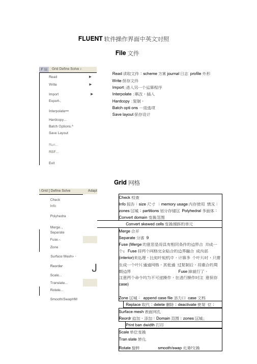
FLUENT 软件操作界面中英文对照File 文件Read 读取文件：scheme 方案journal 日志 profile 外形 Write 保存文件 Import :进入另一个运算程序 Interpolate :窜改，插入Hardcopy :复制，Batch opti ons —组选项Save layout 保存设计 Grid 网格| F 屆 Grid Define Solve i-Read► Write►Import ► Export-, Interpolate —Hardcopy...Batch Options.^Save LayoutRun...RSF...ExitDefine Models模型：solver解算器Pressure based 基于压力Den sity based基于密度末解用丁 pressure based,雀改用Censity based 岀观不苻合秦相36的摄不，请甸pres 羊WE base d Al density based 慎仆则迢.41刊卜 IS 况？北外.血OC ・EHU ^ cotipled ＞（/^ ptiaw ccupl ed simple 可这孔 & pimple ijEpiso 逞划.--■轟=Sortg 冲-丸布时制* ^jfe-5-6 1844DOden ba&ed 亘工F 吋.压聲血ptessurt ba$«i 适可于那可乐册斤"dens Ply based 把丸“河悴掏t ：至殳嗟之一.刑牛可爪門d 的创R 监當歎1一，般如人锻暮叫人丄有用轴怀，火薩墟迭牛才H5）-0 程：yje8D8-丸布门 1叫；20GS-3-7 10-2ODQ歆；I ：谢PrflSsdrfl-Bawd Soker ^Fluflnt 它星英于压力快的束解孤便丹的圮压力修止畀法"求释旳控制片悝足标联式的，擅K 家鮮不町压縮舐Mb 对于町压砂也可旦索麟；Fk«nl 6-3 tl 前的I 板』冷孵臥 B fjS4^r«^at«d &Olvar fli Cfruptod Solvtr,的实也fltje Pr#4iurft-ea5<KJ ScFvAi 约两种虽幵方ib应理拈Fluent 氐J 眇坝犢型小的.它拈垒于曲喪红旳求聲塞，最辑的出H .也桿艮先■那式的.丰誓■載密式冇Roz AU$hk>谏方法的初和&让Fhwrt 耳有比我甘的求IT 可压胃（说劫謹力，們耳帕榕式淮冇琴加IF 科限闾辉，倒比还丰A 完荐匚Coupted 的算送t 对子慨站何Hh 地们足便用円匕口讷油皿购加£未处為性上世魅端计棒低逢刈趾.擁说的DansJty-Bjiwd Solver F ft St SiMPLEC, P 怡DE 些选以的.闪为進些ffliQl ；力修止鼻袪・不金在这种类崖的我押■中氏现泊I 建址祢匹足整用Fw»ur 护P.sed Solver 堺决昧的利底*implicit 隐式， explicit 显示Space 空间：2D , axisymmetric （转动轴）， axisymmetric swirl （漩涡转动轴）；Time 时间 :steady 定常，unsteady 非定常 Velocity formulatio n 制定速度： absolute 绝对的；relative 相对的Gradient option 梯度选择：以单元作基础；以节点作基础；以单元作梯度的最小正方形。

双曲线动能定理的公式

双曲线动能定理的公式英文回答：The formula for the law of conservation of kinetic energy in the context of a hyperbolic motion is given by:KE = 1/2 m v^2。

where KE represents the kinetic energy, m is the mass of the object, and v is the velocity of the object.This formula states that the kinetic energy of an object in motion is directly proportional to the square of its velocity. In other words, as the velocity of an object increases, its kinetic energy increases exponentially.To illustrate this, let's consider the example of a car driving on a highway. Suppose we have two cars, Car A and Car B, with the same mass. Car A is traveling at a velocity of 60 miles per hour, while Car B is traveling at avelocity of 120 miles per hour.Using the formula, we can calculate the kinetic energy for each car:For Car A:KE = 1/2 m (60)^2。

CANopen笔记3--DS402运动控制子协议

CANopen笔记3--DS402运动控制⼦协议 DS301就是⼀个通讯协议栈，DS402是建⽴在DS301基础之上的伺服类控制协议。

协议中规定好每个对象字典值的作⽤，⽐如0x6040，是控制字。

DS402把⼀个伺服控制系统应该具有的功能都定义好了，⼚家和使⽤者按照协议定义即可开发和使⽤符合标准的设备。

NMT NMT是⽹络管理报⽂，⽤于实现⼀些管理操作，⽐如节点重启、进⼊运⾏状态等，⽹络管理状态转换图如下：初始化：设备处于启动状态，不能进⾏通信预运⾏：设备启动完毕，还未进⼊运⾏模式。

设备仅回复SDO、NMT消息运⾏：正常⼯作，可回复SDO、NMT、PDO 停⽌：仅能发送NMT（包括⼼跳消息） NMT报⽂格式很简单，COB-ID固定为0x000，数据为：NMT命令 + 从设备节点ID（0x00表⽰⼴播）Boot-up Messages 设备开机启动完成初始化进⼊预运⾏状态时，会产⽣boot-up事件，发送⼀条boot-up消息。

boot-up消息的COB-ID为：0x700 + Node ID。

假设节点ID为1，则该节点开机后会发送boot-up message（0x00 data, always 0）设备控制根据DS402协议（Chapter 6：Device Control Objects），设备的状态由下图描述。

The device states and possible control sequence of the drive are described by the state machine, as depicted in the following figure: 如上图所⽰，状态机可以分成三部分：“ Power Disabled” (主电关闭)、“ Power Enabled”（主电打开）和“Fault”。

所有状态在发⽣报警后均进⼊“Fault”。

在上电后，驱动器完成初始化，然后进⼊SWITCH_ON_DISABLED状态。

1、下载文档前请自行甄别文档内容的完整性，平台不提供额外的编辑、内容补充、找答案等附加服务。
2、"仅部分预览"的文档,不可在线预览部分如存在完整性等问题,可反馈申请退款(可完整预览的文档不适用该条件!)。
3、如文档侵犯您的权益，请联系客服反馈,我们会尽快为您处理(人工客服工作时间：9:00-18:30)。

Velocity/Position Integration Formula (II):Application to Strapdown Inertial NavigationComputationYuanxin Wu and Xianfei PanAbstract— Inertial navigation applications are usually referenced to a rotating frame. Consideration of the navigation reference frame rotation in the inertial navigation algorithm design is an important but so far less seriously treated issue, especially for the future ultra-precision navigation system of several meters per hour. This paper proposes a rigorous approach to tackle the issue of navigation frame rotation in velocity/position computation by use of the newly-devised velocity/position integration formulae in the Part I companion paper. The two integration formulae set a well-founded cornerstone for the velocity/position algorithms design that makes the compr ehension of the iner tial navigation computation pr inciple mor e accessible to pr actitioner s, and differ ent appr oximations to the integr als involved will give bir th to var ious velocity/position update algorithms. Two-sample velocity and position algorithms are derived to exemplify the design process. In the context of level-flight airplane examples, the derived algorithm is analytically and numerically compared to the typical algorithms existing in the literature. The results throw light on the problems in existing algorithms and the potential benefits of the derived algorithm.Index Ter ms— iner tial navigation, velocity integr ation for mula, position integr ation for mula, fr ame rotationI.I NTRODUCTIONOver fifty years have seen the fruitful algorithm development for the strapdown inertial navigation system using a triad of gyroscopes and accelerometers that are strapped down to the vehicle [1]. Because the inertial sensors rotateThis work was supported in part by the Fok Ying Tung Foundation (131061), National Natural Science Foundation of China (61174002), the Foundation for the Author of National Excellent Doctoral Dissertation of People’s Republic of China (FANEDD 200897) and Program for New Century Excellent Talents in University (NCET-10-0900).Authors’ address: Department of Automatic Control, College of Mechatronics and Automation, National University of Defense Technology, Changsha, Hunan, P. R. China, 410073. Tel/Fax: 086-0731-********-8212 (e-mail: yuanx_wu@).along with the vehicle, the strapdown navigation algorithm is much more complex than that for gimbaled inertial navigation, even worse when a rotating navigation frame is chosen [2-5]. The algorithm researches have been mostly focused on body-related dynamic attitude/velocity/position computation, leading to the state-of-the-art coning/sculling/scrolling corrections that form the basis of the modern strapdown inertial navigation algorithm [1, 4-9]. Though widely believed that the strapdown algorithm has been currently more than adequate, accuracy pursuit is well motivated and objectively necessitated for the on-the-horizon ultra-precision inertial navigation system of several meters per hour [10].Navigation applications are usually referenced to a rotating frame, e.g., the Earth frame or the local level frame. Consideration of the navigation frame rotation in the velocity/position computation is an important algorithm issue for the future ultra-precision navigation system [10], which has so far been less seriously handled in the literature and text books [1-3, 5]. Regarding the attitude computation, the issue can be addressed by the combination of the body frame and the rotating navigation frame both relative to some chosen inertial frame [4]. When it comes to the velocity/position computation, the issue is not as simple as most thought, due to the single/double integrations of the transformed specific force in the velocity/position calculation. To our best knowledge, the first trial treatment was by Savage in [11] with yet little details and then the issue was further investigated in [1, 5] under coarse assumptions. This paper is aimed to propose a rigorous approach to tackle the issue of the navigation frame rotation for velocity and position computation. I t is achieved by use of the velocity integration formula and the position integration formula that are newly derived and applied to the in-flight alignment in the companion paper [12]. Hopefully, the paper will benefit the comprehension of the inertial navigation computation principle1and provide a well-founded systematic framework to design the velocity and position updating algorithms with potentially improved accuracy. This paper, along with the companion paper [12], connects the navigation computation problem and the alignment problem in an interesting way.The remaining of the paper is organized as follows. Section II revisits the velocity/position integration formulae in the incremental form, which sets a solid basis for the velocity/position algorithms design. Section III demonstrates the two-sample velocity/position algorithms derived from the associated integration formula. Simple comparison with existing velocity/position algorithms is performed in the context of level-flight examples in Section I V.1 Somewhat obscurely presented in the classic literature [1, 4, 5], it is difficult to fully understand for non-professionals and even for professionals.Conclusions are drawn in Section V.II.I NCREMENTAL V ELOCITY /P OSITION I NTEGRATION F ORMULAEDenote by N the local level navigation frame, by B the body frame of the inertial navigation system, by I the inertially non-rotating frame, by E the Earth frame. The velocity and position rate equations in the navigation N -frame are respectively known as [1-3]2n n b n n n nb ie en u v C f ȦȦv g (1)n c pR v (2) where n v denotes the vehicle’s velocity relative to the Earth (also called ground velocity), nb C the attitude matrixfrom the body frame to the reference frame, b f the specific force measured by accelerometers in B -frame, n ie Ȧ theEarth rotation rate with respect to the inertial frame, n en Ȧ the angular rate of the navigation frame with respect to the Earth frame, and n g is the gravity vector. The vehicle’s position >@TL h Op is described by the heightabove the Earth surface h and the angular orientation of the navigation frame relative to the Earth frame, commonly expressed as longitude O and latitude L .c R is the local curvature matrix that is a function of the current position. All the quantities above are functions of time and, if not explicitly stated, their time dependences on are omitted for brevity.Next, we will consider the velocity and position updates from time k t to 1k t (1k k t t T ).A.Velocity Integration FormulaBy the chain rule of the attitude matrix, n b C at any timek k k k n tb tn t n t b t b t n t b t C C C C (3)Both the body frame and the navigation frame with respect to any I -frame, sayk b t iC andk n t iC , are functions ofk t instead of t , and hence their time derivatives are zero. To put it the other way, they are inertially “frozen” afterthe time epoch k t passes.Substituting (3) into (1) yields2k k k k n t b t n t n b n nn n ie en b t n t b t u v C C C f ȦȦv g (4)Multiplyingk n t n t C on both sides,2k k k k k kn tn tb tn tn tn b n n nn ie en n t b t n t n t b t u C v C C f C ȦȦv C g (5) Integrating over the time interval of interest,11112k k k k k k k k k k kkkkt t t t n t n t b t n t n tn bn n nn ie enn t b t n t n t b t t t t t dt dt dt dt u ³³³³Cv C Cf CȦȦv C g (6)The term on the left is derived as111111k k k k k k k k k k kkkkt t t t n tn tn tn tn tn n nn n n nn in k k in n t n t n t n t n t t t t t dt dt t t dt u u ³³³C vC v C Ȧv C v v C Ȧv (7) where the attitude rate equation i i n n n inu C C Ȧ is used. The skew symmetric matrix u is defined so that the cross product satisfies u u p q p q for arbitrary two vectors. Substituting (7) into (6) and reorganizing the terms,11111k k k k k k k k k k k k k t t t n t n t b t n t n t n n b nn n k k ie b t n t n t n t b t t t t t t dt dt dt ªº u «»¬¼³³³v C v C C f C Ȧv C g (8)which is the analytic velocity integration formula in the potentially rotating navigation N -frame. Multiplication of the matrix1k k n tn t C depicts the rotating frame effect on the calculation of the velocity during the interval. The secondterm in the bracket k k k kt n t b tb b t b t tdt t ³CC f u is the integration of the transformed specific force that necessitatesthe well-known sculling correction due to the body rotation [1, 5]. The last two terms introduce two new but similar integrals that can be handled by the sculling-like technique to account for the navigation frame rotation. In contrast to (8), previous works unexceptionally reckoned on some kinds of approximation, see e.g., Section 11.3-11.4 in [2], (10) in [5], and (7.2.2-1) and (7.2.2-1a) in [1], and (11.60). These approximations lead to their respective approximate algorithms. Details are provided in (21)-(23) in Section III-A. B.Position Integration FormulaIn the context of a specific local level frame choice, e.g., North-Up-East, the local curvature matrix is explicitly expressed as a function of current position100cos 100010E c N R h L R h ªº«» «»«»«» «»«»«»¬¼R (9)where E R and N R are respectively the transverse radius of curvature and the meridian radius of curvature of the WGS-84 reference ellipsoid. The expression of c R will be different for other local level frame choices, which, however, will not hinder from understanding the main idea of this paper. Clearly, c R will encounter mathematical singularity when the cosine of the latitude approaches zero. In such rare cases, the angular orientation matrix of the navigation frame relative to the Earth frame can be used to encode the longitude and latitude information [1, 2]. It should be highlighted that the following development also applies after a little alternation. As for the position update, integrating (2) from time k t to 1k t gives111k k kkt t n n k k c k c t t t t dt t dt | ³³p p R v p R v (10)where c R is approximately taken as a constant and can be evaluated at, e.g., k t , because the position changes very slowly during the integration interval. For >@1,k k t t t , define the position in N -frame asktn n t t dt ³r v (11)whose rate equation is given asn n rv (12) Note that 0n k t r . The explicit form of n r can be achieved by the similar technique as in deriving the velocity integration formula.Substituting 1k t in (8) by t , (12) yieldsk k k k k k kkkktttn tn tn tb tn tn tn n n b n nn k ie n t n t b t n t n t b t t t t t dt dt dt u ³³³C r C v v C C f C Ȧv C g (13) By the same techniques as in (7),111111k k k k k k k k k k kkkkt t t t n tn tn tn tn tn n nn nn in k in n t n t n t n t n t t t t t dt dt t dt u u ³³³C rC r C Ȧr C r C Ȧr (14)I ntegrating (13) over the time interval >@1,k k t t and substituting (14), we obtain111111k k k k k k k k k k k k k kk kkkkt n t n t n n n k k in n t n t t t t t tt tn t b t n t n t bn nnieb n n b t t t t t t t t T t dtd dt d dt d dt W W W W W W ª u «¬ºu »¼³³³³³³³r C v C Ȧr CCf CȦv Cg (15)which is the analytic position integration formula in the potentially rotating navigation N -frame. It consists of a single integral, the third term in the bracket, of the same structure with those in (8). The first term in the last row11k kt k t t dt I t ³u u is the double integration of the transformed specific force in which the scrolling correctionhas to be applied to account for the body rotation in high-accuracy positioning applications [5]. By analogy, the last two double integrals can be handled by the scrolling-like correction to account for the navigation frame rotation. So far, the position algorithms in the literature all have employed some approximation forms, see e.g. the high-resolution position computation in (76)-(79) in [5].The incremental velocity integration formula (8) and the incremental position integration formula (15) are settled as well-founded analytic cornerstones for the navigation computation algorithm design, and different approximations to the integrals involved will give birth to various velocity and position update algorithms. The velocity/position integration formulae cast the navigation computation algorithm design within a systematic and rather straightforward framework. In contrast to the previous works [1-3, 5], the navigation frame rotation effects are rigorously considered through the two integration formulae.III.D ERIVED V ELOCITY /P OSITION U PDATE A LGORITHMSThis section uses the incremental velocity/position integration formulae as a basis to exemplify the design of the velocity/position update algorithms. Without loss of generality, the update time interval >@1,k k t t is assumed to contain two samples of the gyroscope and accelerometer triads. A.Velocity Update AlgorithmSince nin Ȧ is usually a slowly changing quantity, it is reasonable to approximate the attitude matrix byk n tn n t I | u C ĳ, where n n k in t t | ĳȦ denotes the N -frame rotation vector from k t to the current time. The last two integrals in the velocity integration formula (8) are respectively approximated by11112222k k k kkk k k k k t t n t n nn n nn nniek iniein ie n t t t t t n t n n nn n k in in n t t t T dt I t t dt TI T dt I t t dt TI §·u | u u | u u ¨¸©¹§·| u | u ¨¸©¹³³³³C Ȧv ȦȦv ȦȦv C g Ȧg Ȧg (16)where the quantities n in Ȧ,nie Ȧ,n v and n g are approximately regarded as constants and evaluated at k t . Usingthe two-sample sculling correction, 1k t u is usually approximated by (See the companion paper [12], Appendix A)112121212121223k k n t k b t t §· ' ' ' 'u ' ' 'u ' 'u '¨¸©¹u C v v șșv v șv v ș (17)where 12,''v v are the first and second samples of the accelerometer-measured incremental velocity and12,''șș are the first and second samples of the gyroscope-measured incremental angle, respectively.Substituting into the velocity integration formula (8),1221122k k n t n n n n nn n k k k in ie k in n t T T t t t TI t TI ½§·§·°°| u u u ®¾¨¸¨¸°°©¹©¹¯¿v Cv u ȦȦv Ȧg (18)With the obtained 1n k t v , the second integral in (8) can be refined to give a better approximation. Suppose the velocity changes linearly during >@1,k k t t , i.e.,1n n nn k k k k t t t t t t Tv v v v (19) then the first equation in (16) can be better approximated by1112212212232623k k k kkt t n tnn n nn n n k ie k in ie kk k n t t t n n nn n n n in ie k in ie k k n n nn n n in ie k in ie k t t dt I t t t t t dt T T T T TI t I t t T T T T I t I t §·u | u u ¨¸©¹§·§·| u u u u ¨¸¨¸©¹©¹§·§· u u u u ¨¸¨¸©¹©¹³³C Ȧv ȦȦv v v ȦȦv ȦȦv v ȦȦv ȦȦv (20)Typical approximate velocity algorithms in the literature are presented below for easy reference. Totally ignoring the navigation frame rotation, the velocity algorithm in [2] gave112n n n nn n TN k k k ie en k t t t T t T u v v u ȦȦv g (21)A coarse compensation was proposed in [5], by replacing (6) with (10) therein, as1112n n n n n n nSV k k in k ie en k t t I T t T t T u u v v Ȧu ȦȦv g (22)With the assumptions of constant changingk n t n t C and linearly ramping t u , an improved velocity algorithm in [1,13] was given as1211122k k n t n nn nn n SV k k k ie en k n t t t I t T t Tu v v C u ȦȦv g (23) It can be proved, however, that the above assumptions are rarely satisfied in practice (see Appendix for details). B.Position Update AlgorithmFollowing (16) and noting that 0n k t r , the single integral in the position integration formula (15)10k k kt n tnn in n t t dt u |³C Ȧr (24) The last double integral is approximated by111223226k k k kkkkk kt tt t n t nn nkinn t t t t t k n n k in t n n in d dt I t d dtt t t t I dt T T I W W W W | u §· | u ¨¸¨¸©¹§·| u ¨¸©¹³³³³³Cg Ȧg Ȧg Ȧg (25)Using the linear velocity assumption (19), the second double integral is calculated by11123231232326612312612k k k kkkkt tt tn tnn n n n n nk ie k in ie k k k n t t t t n n nn n n n in ie k in ie k k n n n n in ie k in t d dt I t t t t d dt T T T T T I t I t t T T T T I t I W W W W W §·u | u u ¨¸©¹§·§·| u u u u ¨¸¨¸©¹©¹§·§ u u u ¨¸©¹©³³³³C Ȧv ȦȦv v v ȦȦv ȦȦv v ȦȦv Ȧ1n n ie k t ·u ¨¸¹Ȧv (26)With the two-sample sculling correction, 1k I t u can be approximated by (See the companion paper [12], Appendix B)112111212222551282230k k n t k b t T I t' ' 'u ' 'u ' 'u ' 'u 'u C v v șv șv v șșv (27)Substituting (24)-(26) into the position integration formula (15) yields111232323131261226k k n tn nk k k n t n n n n n nn n in ie k in ie k in t T t I t T T T T T T I t I t I ª| ¬º§·§·§· u u u u u »¨¸¨¸¨¸©¹©¹©¹¼u r C v ȦȦv ȦȦv Ȧg (28) Modeling n t r as a linear function of time with the obtained 1n k t r , the single integral (24) can be refined as12123k k kt n t nnn nn inin in k n t t T T dt I t §·u | u u ¨¸©¹³CȦr ȦȦr (29)Previous works mostly use the position update by, e.g., the trapezoidal integration [2, 3]112n nn TN k k k T t t t r v v (30) By assuming linearly rampingkn t n t I C and t u , a high-resolution position algorithm was proposed in [5] as121111223k k n t n nn n nn SV k k k ie en k k n t T T t T t I t t I t u u rv g ȦȦv C u (31) which was later refined in [1] to122111226k k n t nnn n nn SV k k k ie en k k n t T T t T t I t t I t u u rv g ȦȦv C u (32) The derived velocity/position algorithms in this paper and others aforementioned are summarized in Tables I-II for clear comparison.IV.L EVEL -F LIGHT E XAMPLESThe body rotation-induced algorithm errors are generally overwhelmed over the navigation frame rotation-induced algorithm errors, so we adopt the simple level flight examples in this paper, so as to make the latter kind of errors as much pronounced as possible for better comparison.Let us first consider an airplane carrying with an inertial navigation system that flies level at a constant speed to the east. To make the analysis tractable, the body frame is assumed to be aligned with the local level frame during thewhole flight. For this special level-flight case, the gyroscope-measured body angular rate is b n nn ib in ie en ȦȦȦȦand the accelerometer-measured specific force2b n n n n ie en u f ȦȦv g according to (1). Note that b ib Ȧ andb f are constant here. Consequently, (17) and (27) are respectively specified as 2b b ibT T I §· u ¨¸©¹u Ȧf and 236bb ib T I I T u u Ȧf . Substituting into the velocity algorithms in (18), (21)-(23) gives, respectively,1122212222222222222k k k k n t nn n n n n n n n nn n k k in ie en in ie k in n t n t nn n in in k n t n n nn n in in in in T T T t t TI TI t TI T I T t T T I T I T ½§·§·§·°° u u u u u ®¾¨¸¨¸¨¸°°©¹©¹©¹¯¿§· u u ¨¸©¹§·§·| u u u u ¨¸¨¸©¹©¹v C v ȦȦȦv g ȦȦv Ȧg C ȦȦv ȦȦȦȦv444k nn n k in k t T t t | u v Ȧv (33)212222n nn n nn n TNk k in ie en k n nnk in T t t t T t u u | u vv ȦȦȦv g v Ȧg (34)2112222n nn n nn n SV k k in ie en k n nnk in T t t t T t u u | u vv ȦȦȦv g v Ȧg (35)1211431228k k n t n n nn n SV k k ie en k n t n nn k in k t I t I T t T T t tu | u v C u ȦȦv g v Ȧv (36) where1k k n t n t C are approximated up to two orders of the integration interval. I t shows that, as far as one velocityupdate is concerned for a realistic airplane velocity, the derived algorithm is the most accurate, followed by the algorithm SV2. The other two are the same but with different signs. For this special case, the position algorithm (28) is specified as11212323231223263126122626k k k k n t n n n n n n n k k in ie en n t n n n n n nn n in ie k in ie k in n t n n nin in k n t T t T t I T T T T T T T I t I t I T T I T t ª| u u «¬º§·§·§· u u u u u »¨¸¨¸¨¸©¹©¹©¹¼§· u u ¨¸©¹r Cv ȦȦȦv g ȦȦv ȦȦv Ȧg CȦȦvwhere 1n k t v is replaced by n k t v for simpler comparison. When (29) is incorporated into (15), 1n k t r is refined to12132234k k n t n n n in in k n t n nn k in k TT I I t T T t t §·§· u u ¨¸¨¸©¹©¹| u C ȦȦr v Ȧv (37)The other position algorithms (30)-(32) are respectively specified as1n n TN k k t T t r v (38)21111133223266n k nnn n nn SV k k k ie en k k n k n n n nn n k in ie en k nn nk in T T t T t I t t I t T T t t T T t u u u | u u rv g ȦȦv C u v ȦȦȦv g v Ȧg (39)122111535322622424k k n t n nn n nn SV k k k ie en k k n t n n n nn n k in ie en k nn n k in T T t T t I t t I t T T t t T T t u u u | u u rv g ȦȦv C u v ȦȦȦv g v Ȧg(40) As far as one position update is concerned in the considered example, the algorithm TN runs as the most accurate one, followed by SV2, the derived one and SV1in the accuracy-descending order. The specific velocity and position algorithms for the level-flight const-speed example are listed in the right columns of Tables I-II.The above level-flight example is simulated for an hour with an east velocity 500 m/s at latitude 30Ϩ. The algorithm update interval is set to 0.02T s , with no vertical damping applied. The horizontal velocity errors and horizontal position errors for each algorithm are plotted in Figs. 1-2, respectively. The algorithms TN and SV1 come with the same largest error behaviors, with the maximum position error of over ten meters. The derived algorithm shows the smallest error in both velocity and position, tightly followed by SV2. I t should be emphasized that an infinitely small number 2010 is used in Fig. 2 to represent the actual zero in the simulation result and the suddenjump of SV2 at about 2800s is owed to the numerical truncation error. I n this case, 41.610ninu Ȧ and0.0014b b b b b ib ibu |u Ȧf f Ȧf . The assumptions in SV2 (see (41)-(42))are roughly satisfied. We further simulated and examined another level flight example with the east velocity rate sin n E a wt v .When the rate magnitude 10a and the rate angular frequency 0.02w S , the east velocity profile at 0-300s is plotted in Fig. 3. The horizontal velocity and position errors (2-hour) for each algorithm are respectively given in Figs. 4-5. The derived algorithm is significantly the smallest in both velocity and position errors, followed by SV2, TN and SV1 in the accuracy-descending order. We have also performed many other simulations by changing the velocity rate’s magnitude and angular frequency, and the rank result is quite similar. For such an example, it can beshown that4max 2.210n in u Ȧ andmax max 0.63b b b b ib u | Ȧf ff , the latter of which badly violates the second assumption (42). It explains the unsatisfying behavior of SV2in Figs. 4-5.V.C ONCLUSIONSNavigation frame rotation is an important issue that should be well-considered in the future ultra-precision inertial navigation algorithm design, but has been less seriously handled so far. I n this paper, the velocity and position integration formulae are employed to rigorously tackle the navigation frame rotation issue. In doing so, the inertial navigation velocity/position algorithms design is cast into a systematic and straightforward framework that hopefully benefits the comprehension of the inertial navigation computation principle. Different approximations to the integrals involved in the velocity/position integration formulae give birth to various velocity/position update algorithms. Two-sample velocity and position algorithms are derived to demonstrate the design process within the framework. In the context of level-flight airplane examples, the derived algorithm is analytically and numerically compared to the typical navigation algorithms in the literature. Significant benefits of the derived algorithms are observed.A PPENDIXHere we dwell upon the assumptions in deriving the velocity algorithm SV2 in [1].Sincek k n t n t n in n t n t u C ȦC and rigid rotations do not change the length of a vector, “constant chang ingk n t n t C ” means2200k k k n t n t n t n n in in n t n t n t nn ininu u u u C ȦC ȦC ȦȦ(41)which is satisfied when 0nin Ȧ, namely, N -frame is an inertial frame.Similarly, sincek k b tb t b ib b t b t u C C Ȧ andk k kn t b t b b t b t t u C C f (see the text below (8) for t u ’s definition), “linearly ramping t u ”means00k k k k kk n tb tn tb tb bb ib b t b t b t b t b bbibt u u u C C Ȧf C C f Ȧf f(42)which is valid only under rare conditions, for example, when the INS is rotated with zero origin translation (see (21) in [14]).A CKNOWLEDGEMENTSSpecial thanks to the audiences of the university Graduate Course “Autonomous Navigation and Its Applications” in Spring 2011, who inspire the authors to consider the subject of this paper in a more serious manner.R EFERENCES[1] P. G . Savage, Strapdown Analytics , 2nd ed.: Strapdown Analysis, 2007.[2]D. H. Titterton and J. L. Weston, Strapdown Inertial Navig ation Technolog y : the I nstitute of Electrical Engineers, London, United Kingdom, 2nd Ed., 2004.[3]P. D. Groves, Principles of GNSS, Inertial, and Multisensor Integrated Navigation Systems : Artech House, Boston and London, 2008.[4]P. G . Savage, "Strapdown inertial navigation integration algorithm design, part 1: attitude algorithms," Journal ofGuidance, Control, and Dynamics, vol. 21, pp. 19-28, 1998.[5]P. G . Savage, "Strapdown inertial navigation integration algorithm design, part 2: velocity and position algorithms,"Journal of Guidance, Control, and Dynamics, vol. 21, pp. 208-221, 1998.[6]D. A. Tazarts, "Inertial Navigation: From Gimbaled Platforms to Strapdown Sensors," IEEE Trans. on Aerospace andElectronic Systems, vol. 47, pp. 2292-2299, 2011.[7] Y . Wu , et al., "Strapdown inertial navigation system algorithms based on dual quaternions," IEEE Transactions on。