Improved model to solve influence coefficients of work roll deflection
Kaplan-Meier多重估计的竞争风险环境分析中的累积病率函数恢复失效信息说明书

Package‘kmi’October13,2022Version0.5.5Title Kaplan-Meier Multiple Imputation for the Analysis of CumulativeIncidence Functions in the Competing Risks SettingAuthor Arthur Allignol<*************************>Maintainer Arthur Allignol<*************************>Imports mitools,survival,statsDescription Performs a Kaplan-Meier multiple imputation to recover the missing potential censor-ing information from competing risks events,so that standard right-censored meth-ods could be applied to the imputed data sets to perform analyses of the cumulative inci-dence functions(Allignol and Beyersmann,2010<doi:10.1093/biostatistics/kxq018>). License GPL(>=2)URL https:///aallignol/kmiBugReports https:///aallignol/kmi/issuesNeedsCompilation noRepository CRANDate/Publication2019-05-2721:10:13UTCR topics documented:cox.kmi (2)icu.pneu (3)kmi (4)print.cox.kmi (7)print.summary.cox.kmi (7)summary.cox.kmi (8)Index1012cox.kmi cox.kmi Cox proportional hazards model applied to imputed data setsDescriptionThis functionfits Cox proportional hazards models to each imputed data set to estimate the regres-sion coefficients in a proportional subdistribution hazards model,and pools the results.Usagecox.kmi(formula,imp.data,plete=Inf,...)Argumentsformula A formula object,with the response on the left of a~operator,and the terms on the right.The response must be a survival object as returned by the Survfunction.imp.data An object of class kmi.plete Complete data degrees of freedom....Further arguments for the coxph function.DetailsFits a Cox proportional hazards model on each imputed data set to estimate the regression coeffi-cients in a proportional subdistribution hazards model,and pools the results,using the MIcombine function of the mitools package.ValueAn object of class cox.kmi including the following components:coefficients Pooled regression coefficient estimatesvariance Pooled variance estimatenimp Number of multiple imputationsdf degrees of freedomcall The matched callindividual.fit A list of coxph objects.One for each imputed data set.Author(s)Arthur Allignol,<*************************>See Alsocoxph,MIcombine,print.cox.kmi,summary.cox.kmiicu.pneu3Examplesdata(icu.pneu)if(require(survival)){set.seed(1313)imp.dat<-kmi(Surv(start,stop,status)~1,data=icu.pneu,etype=event,id=id,failcode=2,nimp=5)fit.kmi<-cox.kmi(Surv(start,stop,event==2)~pneu,imp.dat)summary(fit.kmi)###Now using the censoring-complete datafit<-coxph(Surv(start,adm.cens.exit,event==2)~pneu,icu.pneu)summary(fit)##estimation of the censoring distribution adjusted on covariatesdat.cova<-kmi(Surv(start,stop,status)~age+sex,data=icu.pneu,etype=event,id=id,failcode=2,nimp=5)fit.kmi2<-cox.kmi(Surv(start,adm.cens.exit,event==2)~pneu+age,dat.cova)summary(fit.kmi2)}icu.pneu Hospital acquired penumonia in ICUDescriptionThis data set is a random sample drawn from the SIR-3study that aimed at analysing the effect of nosocomial infections on the length of ICU stay.Patients were included in the study if they had stayed at least1day in the unit.The sample includes information to assess the effect of nosocomial pneumonia on the length of stay.The endpoint is either discharge alive from the ICU or dead in the unit.These data are censoring complete as the censoring time is known for all patients.Usagedata(icu.pneu)FormatA data frame with1421observations on the following8variables.4kmiid Individual patient id.start Start of the observation time.stop Failure time.status Censoring status.0if the observation is censored,1otherwise.event Event type.2is death in ICU,3is discharge alivepneu Nosocomial pneumonia indicator.adm.cens.exit Exit times for patients discharged alive are replaced by their administrative cen-soring times.age Age at inclusionsex Sex.F for female and M for maleSourceBeyersmann,J.,Gastmeier,P.,Grundmann,H.,Baerwolff,S.,Geffers,C.,Behnke,M.,Rueden,H., and Schumacher,e of multistate models to assess prolongation of intensive care unit stay due to nosocomial infection.Infection Control and Hospital Epidemiology,27:493-499,2006.ReferencesBeyersmann,J.and Schumacher,M.(2008).Time-dependent covariates in the proportional hazards model for competing risks.Biostatistics,9:765–776.Examplesdata(icu.pneu)kmi Kaplan-Meier Multiple Imputation for Competing RisksDescriptionThe function performs a non parametric multiple imputation that aims at recovering the missing potential censoring times from competing events.Usagekmi(formula,data,id=NULL,etype,failcode=1,nimp=10,epsilon=1,bootstrap=FALSE,nboot=10)kmi5Argumentsformula A formula object,that must have a Surv object on the left of a~operator.Covariates could be added on the right hand side of the formula.They will beused to model the censoring distribution.See Details.data A data.frame in which to interpret the variables given in the formula,etype and id.It is mandatory.id Used to identify individual subjects when one subject can have several rows of data,e.g.,with time-dependent covariates.Set to NULL when there is only oneraw of data per subject.etype Variable specifying the type of competing event.When status==1in formula, etype describes the type of event,otherwise,for censored observation,(status==0),the value of etype is ignored.failcode Indicates the failure cause of interest.Imputation will be performed on the other competing events.Default is1.nimp Number of multiple imputation.Default is10.epsilon When the last time is an event,a censoring time equal to max(time)+epsilon is added.By default,epsilon is set to1.bootstrap Logical.Whether to estimate the censoring distribution using bootstrap samples.Default is FALSE.nboot If bootstrap is set to TRUE,nboot determines the number of bootstrap sam-ples.DetailsIt was shown that if censoring times are observed for all individuals,methods for standard right-censored survival data can be used to analyse cumulative incidence functions from competing risks (Fine and Gray1999).Therefore the idea proposed by Ruan and Gray(2008)is to impute potential censoring times for individuals who have failed from the competing events.The censoring times are imputed from the conditional Kaplan-Meier estimator of the censoring distribution.Estimation of the censoring distribution may be improved through bootstrapping.Estimation might also be improvedfitting a model for the censoring distribution.When covariates are given,a pro-portional hazards model on the hazard of censoring isfit.The censoring times are then imputed from the estimated model.The competing risks model formulation in formula mimics the one in survfit.ValueAn object of class kmi with the following components:imputed.data A list of matrices giving the imputed times in thefirst column and imputed event type in the second column.The event status for imputed times take value0(censored).original.data The original data setinfo Gives the names of the time and event indicator column in the original data set.call The matched call.6kmiWarningWhen a proportional hazards model isfit for modelling the censoring distribution,the censoring times are imputed from the imputed model.When there is missing covariate information for the prediction,mean imputation is used.NoteThis multiple imputation technique does not work for left-truncated data.Author(s)Arthur Allignol,<*************************>ReferencesRuan,P.K.and Gray,R.J.(2008).Analyses of cumulative incidence functions via non-parametric multiple imputation.Statistics in Medicine,27(27):5709–5724.Allignol,A.and Beyersmann,J.(2010).Software forfitting nonstandard proportional subdistribu-tion hazards models.Biostatistics,doi:10.1093/biostatistics/kxq018Fine,J.P.and Gray,R.J.(1999).A Proportional Hazards Model for the Subdistribution of a Com-peting Risk.Journal of the American Statistical Association.94(446):496–509.See Alsoicu.pneu,cox.kmi,Surv,survfitExamplesdata(icu.pneu)if(require(survival)){dat<-kmi(Surv(start,stop,status)~1,data=icu.pneu,etype=event,id=id,failcode=2,nimp=5)##another way to specify the formula if there is no status##variableicu.pneu$ev<-icu.pneu$eventicu.pneu$ev[icu.pneu$status==0]<-0dat<-kmi(Surv(start,stop,ev!=0)~1,data=icu.pneu,etype=ev,id=id,failcode=2,nimp=5)##with covariates to model the censoring distributiondat.cova<-kmi(Surv(start,stop,status)~age+sex,data=icu.pneu,etype=event,id=id,failcode=2,nimp=5)}print.cox.kmi7 print.cox.kmi Print method for cox.kmi objectsDescriptionPrint method for cox.kmi objects.Usage##S3method for class cox.kmiprint(x,print.ind=FALSE,...)Argumentsx An object of class cox.kmi.print.ind A logical specifying whether to print the results of the analyses performed on each imputed data set.By default,only the pooled estimates are printed....Further argumentsValueNo value returnedAuthor(s)Arthur Allignol,<*************************>See Alsocox.kmi,summary.cox.kmiprint.summary.cox.kmi Print method for summary.cox.kmi objectsDescriptionPrint method for summary.cox.kmi objects.Usage##S3method for class summary.cox.kmiprint(x,digits=max(getOption("digits")-3,3),signif.stars=getOption("show.signif.stars"),print.ind=FALSE,...)Argumentsx An object of class summary.cox.kmi.digits Significant digits to print.signif.stars Logical.If TRUE,’significance stars’are printed for each coefficient.print.ind Logical specifying whether to print a summary of the modelsfitted on each imputed data set.Default is FALSE...Further argumentsValueNo value returnedAuthor(s)Arthur Allignol,<*************************>See Alsosummary.cox.kmisummary.cox.kmi Summary method for cox.kmi objectsDescriptionProvides a summary of thefitted model.Usage##S3method for class cox.kmisummary(object,conf.int=0.95,scale=1,...)Argumentsobject An object of class cox.kmi.conf.int Level of the confidence intervals.Default is0.95scale Vector of scale factors for the coefficients,default to1.The confidence limits are for the risk change associated with one scale unit....Further argumentsValueAn object of class summary.cox.kmi with the following components:call The matched callcoefficients A matrix with5columns including the regression coefficients,subdistribution hazard ratios,standard-errors,t-statistics and corresponding two-sided p-values.conf.int A matrix with4columns that consists of the subdistribution hazard ratios,exp(-coef)and the lower and upper bounds of the confidence interval.individual.fit A list of summary.coxph objects for each imputed data setAuthor(s)Arthur Allignol,<*************************>See Alsocox.kmi,print.summary.cox.kmi,summary.coxphIndex∗datasetsicu.pneu,3∗methodssummary.cox.kmi,8∗modelscox.kmi,2∗printprint.cox.kmi,7print.summary.cox.kmi,7∗regressioncox.kmi,2∗survivalcox.kmi,2kmi,4cox.kmi,2,6,7,9coxph,2icu.pneu,3,6kmi,4MIcombine,2print.cox.kmi,2,7print.summary.cox.kmi,7,9summary.cox.kmi,2,7,8,8summary.coxph,9Surv,2,6survfit,5,610。
一个优化问题的辅助模型解法

一个优化问题的辅助模型解法
刘坤会
【期刊名称】《北方交通大学学报》
【年(卷),期】1992(016)001
【摘要】本文借助一类最佳停止问题的费用函数,研究了一类推广的奇异型折扣费用问题,在其主要控制区域中证明了折扣费用模型最佳控制存在并刻划出其结构.【总页数】13页(P40-52)
【作者】刘坤会
【作者单位】无
【正文语种】中文
【中图分类】O211.64
【相关文献】
1.套产品下料模型及其辅助模型解法 [J], 樊治平
2.一类转库问题流向优化问题的模型与解法 [J], 高天;王梦光;唐立新;宋建海
3.一个无约束最优化问题的计算机解法 [J], 王玉;杨秀珍
4.代理模型辅助进化算法在高维优化问题中的应用 [J], 田杰;谭瑛;孙超利;曾建潮
5.高计算代价动态优化问题的代理模型辅助粒子群优化算法 [J], 张勇;胡江涛因版权原因,仅展示原文概要,查看原文内容请购买。
IEEE pdf版本

A Novel Model for Implementation of GammaRadiation Effects in GaAs HBTs Jincan Zhang,Yuming Zhang,Senior Member,IEEE,Hongliang Lu,Member,IEEE,Yimen Zhang,Senior Member,IEEE,and Min LiuAbstract—For predicting the effects of gamma radiation on gal-lium–arsenide(GaAs)heterojunction bipolar transistors(HBTs), a novel model is presented in this paper,considering the radiation effects.Based on the analysis of radiation-induced degradation in forward base current and cutoff frequency,three semiempirical models to describe the variation of three sensitive model parame-ters are used for simulating the radiation effects within the frame-work of a simplified vertical bipolar inter-company model.Its va-lidity was demonstrated by analysis of the experimental results of GaAs HBTs before and after gamma radiation.Index Terms—Cutoff frequency,forward base current,gamma radiation effects,heterojunction bipolar transistor(HBT),semi-conductor device modeling,vertical bipolar inter-company (VBIC).I.I NTRODUCTIONG ALLIUM–ARSENIDE(GaAs)heterojunction bipolartransistors(HBTs),due to their superior performance, are widely used in space radiation environments,and the recent boost of wireless and other high-end communications continue to draw more and more attention to its reliable long-term per-formance under radiation.Earlier studies on radiation effects on GaAs HBT have shown that GaAs HBTs are very attractive candidates for applications in space-based communication sys-tems[1],[2].In this case,many integrated circuits(ICs)have been designed with a GaAs HBT process[3]–[5].However, to improve the radiation hardness of HBT ICs,designers need electrical models taking account for the degradation induced by radiation.However,most of the radiation studies on GaAs HBTs re-ported thus far have mainly focused on the radiation induced changes from the experimental results with the measured elec-trical characteristics of the devices(e.g.,excess base current, cutoff frequency,etc.)[1],[2],[6],[7].To our knowledge,there is not much published information on modeling the electrical characteristics of HBTs subjected to high-energy radiations[8]. The work of modeling the effects of gamma radiation on the dc characteristics of GaAs HBTs has been studied in our pre-vious work[9].However,the complexity of the radiation-in-Manuscript received May03,2012;revised September16,2012;accepted September20,2012.This work was supported by the National Basic Research Program of China under Grant2010CB327505,the Advance Research Project of China under Grant51308030306,and the Advance Research Foundation of China under Grant9140A08030511DZ111.The authors are with the Microelectronics Institute,Xidian University,Xi’an, Shaanxi710071,China(e-mail:zjc850126@).Digital Object Identifier10.1109/TMTT.2012.2221137duced degradation processes makes it difficult to develop a de-tailed physical model of the device after radiation.An alter-native semiempirical approach is to develop an improved ver-tical bipolar inter-company(VBIC)model to describe electrical characteristics of the device before and after irradiation.One can use the extracted model parameters to describe the degra-dation of sensitive model parameters as a function of radiation dose,and then assemble the device model.We believe that such an approach is very useful to predict the degradation effects of devices.There were reports for simulating radiation-induced degradation of dc characteristics in bipolar transistors of silicon based on the semiempirical approach[10],[11].However,very little progress has been made in modeling the degradation of ac characteristics as a function of radiation dose in bipolar transis-tors based on the semiempirical approach,which is now studied in this work.In this paper,a novel model for implementation of gamma ra-diation effects in GaAs HBTs is developed.This paper is orga-nized as follows.The novel model based on a simplified VBIC model is presented in Section II.To validate the validity of the model,the experimental results of GaAs HBTs under gamma radiation are shown in Section III.The modeled results are com-pared with the measured results in Section IV and conclusions are presented in Section V.II.M ODELThe VBIC model was defined by a group of representa-tives from IC and computer-aided design(CAD)industries to overcome the shortcomings of the Spice Gummel Poon(SGP) model.The equivalent network of VBIC is given in[12].There are several improvements comparing with the SGP model, such as temperature-dependence modeling,quasi-saturation modeling,and decoupling of base and collector currents. However,special characteristics of HBTs make it possible to consider a simplified VBIC model,as shown in Fig.1.In this simplified VBIC model,the following assumptions are consid-ered.1)There is no parasitic pnp transistor in npn HBTs[13];there-fore,the parameters to describe the parasitic transistor can be eliminated.2)The extrinsic base–emitter current and chargecan be neglected compared to the intrinsic base–emitter current and charge,respectively.3)Since de-embedding the parasitic parameters has beendone,base–collector small-signal capacitance and base–emitter small-signal capacitance can be ig-nored.0018-9480/$31.00©2012IEEEFig.1.Simplified VBIC model.4)In HBTs,both early voltages and knee currents for the for-ward and reverse operations can be considered to be infi-nite[14],therefore the normalized base charge tends to be1.The validity of the model to describe HBTs characteristics has been verified in our earlier work[15].Unfortunately,the simplified VBIC model also has not taken account of the par-ticular effects of radiation on the electrical behavior of devices. However,HBTs are significantly degraded when exposed to ra-diation.Forward base current and cutoff frequency are mainly affected.A.Forward Base CurrentIn the measurement of forward-mode Gummel plot,the base current is measured when isfixed at zero while the base–emitter junction is in forward bias.The presence of the relatively large valence band discontinuity at the base–emitter heterointerface leads to effective suppression of the hole current injected from the base region into the emitter.Thus,the base current is mostly determined by the recombination of:1)in the bulk and along the periphery of the base–emitter space-charge region(BE-SCR)and2)in the bulk and at the surface of the neutral base region(NBR).In the simplified VBIC model,the total forward base current for low-level injection where voltage drop across parasitic re-sistances can be neglected is followed by(1) where is the thermal voltage.As can be seen from (1),the base current includes a component,formed by the NBR recombination modeled with saturation current and ideality factor,and a component,caused by the BE-SCR recombination modeled with saturation currentand ideality factor.Radiation-induced degradation in the forward base current of HBTs is attributed to excess carrier recombination including ra-diation-induced traps in the BE-SCR[9],whereas excess base current defined as the difference between the post-radi-ation and pre-radiation base current can be experimentally ex-tracted by the variations of and with radiation dose. In this case,(1)will be improved as(2),in which radiation-in-duced excess saturation current and excess ideal factor are included.(2)B.Cutoff FrequencyPhysically,can be expressed as(3)(4)(5) where is the base–emitter junction capacitor charge time,is the base–collector junction capacitor charge time,is the base transit time,and is the base–collector space-charge region delay time.It has been shown that capacitance and resistance are slightly or even not degraded under radiation for HBTs in our previous works[16],Therefore,the degradation of is mainly caused by the increase of the transit time,which is just the sum of the variations of and in the compact model[17].In the simplified VBIC model,the transit time is modeled as(6) where is the forward transit time,is the variation of with basewidth modulation,is the coefficient of bias dependence,is the coefficient of dependence on, is the coefficient of dependence on,and is the forward collector current.Inserting a parameter related to the variation of due to radiation effect,the equation of the transit time can be im-proved as(7) where radiation-induced excess forward transit time is used to predict the increase of,in turn to describe the degra-dation of.III.E XPERIMENTSIn order to determine the regulations of,,and with radiation dose,and verify the validity of the presented model,the following radiation experiment has been performed.ZHANG et al.:NOVEL MODEL FOR IMPLEMENTATION OF GAMMA RADIATION EFFECTS IN GaAs HBTs3Fig.2.Radiation-induced degradation of base current for different total dose levels.The devices applied in the experiment are GaAs HBTs with a single fabrication batch from the WIN Semiconductors Corpo-ration,Tao Yuan Shien,Taiwan(type Q1H201B1).The width and length of each emitter mesa for Q1H201B1are1and20 m,respectively.Radiation of devices,without bias,was im-plemented in a“Gamma-Cell”with a Co source providing a dose rate of about50rd(Si)/s rd Si rd GaAs, and radiation time of5.5,16.5,38.5,and55h,equivalent to a gamma total dose of1,3,7,and10Mrd(Si),respectively.In order to get enough accurate test data,there were four test sam-ples under every radiation total dose mentioned above.Before the experiment,the samples were carefully selected to ensure the differences of performances among the16tested HBTs to be less than3%and the spread of the measured data for the four devices at each radiation to be within0.1%.All of samples were measured at room temperature K before and after radiation.On-chip forward dc Gummel characteristic measure-ments were made with an HP4142Semiconductor Analyzer. Scattering parameters(-parameters)were measured using an HP8510C vector network analyzer from100MHz to40GHz, and in a wide bias current range based on circuit applications.A.Forward Base CurrentFig.2shows the plot of measured versus with the base–collector junction shorted for different total dose radiation, while the collector current remains approximately unchanged. As can be seen from thisfigure,at low current levels,the curve shows significant change after radiation.In the high current regime,almost has no change.The increase rate of base current,defined as the ratio of excess base current to pre-radiation base current,is plotted with incremental dose values,as shown in Fig.3.The increase rate increases with the total dose,and reaches620%at V after a gamma total dose of10Mrd(Si).However,as can be seen from Fig.3,the increase rate of base current versus decreases.In the regime of V,the increase rate becomes close to0.Fig.4shows the effect of the total dose on the excess base current for different total dose levels.The results presented are limited in the low injection current region where the excess base current remains significant compared with thevalue of the total base current.The excess basecurrent is approximately linear throughout the biasrange with a slope of the idea factor Fig.3.Increase rate of forward base current.Fig.4.Radiation-induced excess base current.Fig.5.versus collector current for different total dose levels..These results indicate that radiation-induced recombi-nation mechanism in the BE-SCR is more dominant in the ex-cess base current.Thus,it is reasonable that only the and parameters associated with the BE-SCR are improved in the novel model,as shown in(2).There are two possible recombination mechanisms in the BE-SCR to be consistent with the measured base current ide-ality factor[18].One is trap-assisted tunneling due to gamma radiation induced traps.The second possible mecha-nism is the recombination from a nonuniform distribution of Shockley–Read–Hall centers within the BE-SCR.B.Cutoff FrequencyThe cutoff frequency was extracted using-parameters measurements in the common-emitter configuration by extrap-olating.Fig.5shows measured versus collector current for different total dose levels.In general,relatively obvious degradation is observed for the GaAs HBT after10-Mrd(Si)ra-diation.4IEEE TRANSACTIONS ON MICROWA VE THEORY ANDTECHNIQUESing fly-backing fly-back measurement.The emitter series resistance was measured with the fly-back technique in which the emitter is grounded and current is forced into the base.The open circuit collector voltage was measured.The emitter resistance is taken as the slope of the linear segment of the curve.Fig.6shows the comparison of from fly-back measurement curves before and after 10-Mrd(Si)radiation.As can be seen from this figure,there is almost no change in .In the simpli fied VBIC model,includes the extrinsic col-lector resistance and intrinsic collector resistance .Fig.7shows from fly-back measurement curves to be similar to measurement.The value of is equal to the slope of the linear segment of the curve,and has no change after radiation.can be determined by optimizing the fitting to quasi-saturation region data of common-emitter char-acteristics.It can then be obtained that there is almost no change in .The possible reason for almost unchanged and after radiation is that the doped concentration in HBT devices is high,which makes radiation induced a little reduction of carrier con-centration causing no obvious increment in and .Fig.8shows the comparison of the capacitances for the GaAs HBT.The curves nearly coincide,suggesting that even after 10-Mrd(Si)total dose gamma radiation,the capacitances almost do not change.According to the measured results,it can be concluded that the degradation of is only due to the change of ,which validates the correctness of the discussion in Section II-B.IV .A NALYSIS AND D ISCUSSIONTo predict the electrical behavior of ICs for a given radiation total dose,designers usually need an ef ficient evaluation oftheFig.8.Capacitances (and )for GaAs HBT.TABLE I V ALUES OF,,,AND P ARAMETERS FOR P RE -R ADIATIONAND P OST -R ADIATION OF D IFFERENT R ADIATION L EVELSradiation parameters embedded in sensitive device model pa-rameters to determine the degradation of these parameters with dose.Such an approach permits an easy implementation for ra-diation-induced degradation in the electrical simulator,such as the Advanced Design System (ADS),by means of symbolically de fined device (SDD),which is an equation-based module to en-able designer to quickly and easily de fine custom and nonlinear components.Furthermore,this approach,which allows reason-able computation time,is generally preferred for the applica-tions of complex physics with large numbers of parameters.A.Forward Base CurrentTo extract the forward Gummel base current parameters,theand parameters can be determined from the inter-cept and the slope of the plot in the region of low .The values of and are then easily obtained by fitting the curve in the high injection region.The obtained ,,,and parameter values are listed in Table I for pre-radiation and post-radiation of different radiation levels.The extracted curves for and versus total dose are plotted in Fig.9(a)and (b),respectively.A saturation effect is exhibited for high total doses.The objective functions for fitting and are shown in (8)and (9),respec-tively,where Dose represents the gamma radiation total dose [in Mrd(Si)]and ,,,,,and are fitting parametersDose (8)Dose(9)As can be seen from Fig.9(a)and (b),the fitting curves of the first four dose levels (first four modeled)nearly coincide with that of all the five dose levels (modeled).The values of and at Dose Mrd(Si)obtained from the first four modeled,modeled,and measured are shown in Table II.ThereZHANG et al.:NOVEL MODEL FOR IMPLEMENTATION OF GAMMA RADIATION EFFECTS IN GaAs HBTs5(a)(b)Fig.9.(a)Comparison of the measured and modeled.(b)Comparisonof the measured and modeled.TABLE IIVALUES OFANDP ARAMETERS AT DoseMrd(Si)parison of the measured and first four modeled excess base cur-rent for 10-Mrd(Si)gamma radiation.are little deviations between the measured values and the firstfour modeled values.The error between the measured excess base current and the excess base current based on first four modeled is less than 5%for the fifth total dose 10Mrd(Si),as depicted in Fig.10.Thus,it can be concluded that the novel model should be able to pre-dict accurately the radiation-induced degradation in excess base current even after more than 10-Mrd(Si)gammaradiation.The measured and modeled forward base current for dif-ferent total doses is drawn in Fig.11.The modeled results parison of the measured and modeled forward base current for different total dose levels.TABLE IIIV ALUES OF,,,,AND P ARAMETER FOR P RE -R ADIATION AND P OST -R ADIATION OF D IFFERENT R ADIATION L EVELSmatch the measured data reasonably well (the error within 2%)up to V.The difference between the measured and modeled increases up to 3%for the high injection current region because our model does not account for the degradation of the NBR.However,this mismatch is still not bad.B.Cutoff FrequencyIn order to extract the transit time parameters,the forward transit time is obtained from the intercept of against the curve.The ,,,and param-eters of the transit time are further estimated by optimization.Table III presents the extracted ,,,,and parameter values for pre-radiation and post-radiation of dif-ferent radiation levels.It seems that parameters do not change much between pre-radiation and post-radiation.Since the most susceptible transistor materials to be sensitive to the total dose effect are insulators,the SiN insulator instead of oxides in the GaAs HBTs does not show serious degradation to the total dose effect.To describe the decrease of ,the following objective func-tion is used to describe excess forward transit time :Dose(10)where ,,and are fitting parameters.The measured and modeled versus total dose is pre-sented in Fig.12.The fitting curve based on the first four dose levels almost entirely coincides with that based on all five dose levels,suggesting that the novel model should be able to predict the degradation of cutoff frequency under more than 10-Mrd(Si)gamma radiation.The cutoff frequency versus is illustrated in Fig.13for different total dose levels with a maximum error less than 1%in the all-bias range.6IEEE TRANSACTIONS ON MICROWA VE THEORY ANDTECHNIQUESparison of the measured and modeled.parison of the measured and modeled cutoff frequency for dif-ferent total dose levels.V .C ONCLUSIONA novel model to include total dose effects for HBTs has been presented in this paper.To predict the behavior of ICs in space-like environments,semiempirical models for radiation parameters as a function of radiation total dose have been pro-posed.By incorporating the radiation parameters into sensitive model parameters,a novel model based on a simpli fied VBIC model has been implemented to simulate accurately the radia-tion-induced degradation in forward base current and cutoff fre-quency at least 10-Mrd(Si)gamma total dose.Our analysis also shows that the model can possibly predict the electrical charac-teristics of HBTs even more than 10-Mrd(Si)gamma radiation;however,further experimental study is required to prove the de-duction.R EFERENCES[1]S.M.Zhang,G.F.Niu,J.D.Cressler,S.J.Mathew,U.Gogineni,S.D.Clark,P.Zampardi,and R.L.Pierson,“A comparison of the effects of gamma radiation on SiGe HBT and GaAs HBT technologies,”IEEE Trans.Nucl.Sci.,vol.47,no.6,pp.2521–2527,Dec.2000.[2]S.Vuppala,C.S.Li,P.Zwicknagl,and S.Subramanian,“Neutron,proton and electron radiation effects in InGaP/GaAs single hetero-junc-tion bipolar transistors,”IEEE Trans.Nucl.Sci.,vol.50,no.6,pp.1846–1851,Dec.2003.[3]U.Karthaus,D.Sukumaran,S.Tontisirin,S.Ahles,A.Elmaghraby,L.Schmidt,and H.Wagner,“Fully integrated 39dBm,3-stage doherty PA MMIC in a low-voltage GaAs HBT technology,”IEEE Microw.Wireless Compon.Lett.,vol.22,no.2,pp.94–96,Feb.2012.[4]N.G.Constantin,P.J.Zampardi,and M.N.El-Gamal,“Automatichardware recon figuration for current reduction at low power in RFIC PAs,”IEEE Trans.Microw.Theory Techn.,vol.59,no.6,pp.1560–1570,Jun.2011.[5]K.Yamamoto,H.Kurusu,S.Suzuki,and M.Miyashita,“High-direc-tivity enhancement with passive and active bypass circuit techniques for GaAs MMIC microstrip directional couplers,”IEEE Trans.Mi-crow.Theory Techn.,vol.59,no.12,pp.3095–3107,Dec.2011.[6]E.P.Wilcox,S.D.Phillips,P.Cheng,T.Thrivikraman,A.Madan,J.D.Cressler,G.Vizkelethy,P.W.Marshall,C.Marshall,J.A.Babcock,K.Kruckmeyer,R.Eddy,G.Cestra,and B.Y.Zhang,“Single event transient hardness of a new complementary npn pnp SiGe HBT technology on thick-film SOI,”IEEE Trans.Sci.,57,no.6,pp.3293–3297,Dec.2010.[7]S.Díez,M.Lozano,G.Pellegrini,F.Campabadal,I.Mandic,D.Knoll,B.Heinemann,and M.Ullán,“Proton radiation damage on SiGe:C HBTs and additivity of ionization and displacement effects,”IEEE Trans.Nucl.Sci.,vol.56,no.4,pp.1931–1936,Aug.2009.[8]M.V.Uffelen,S.Geboers,P.Leroux,and F.Berghmans,“Spice mod-elling of a discrete COTS SiGe HBT for digital applications up to MGy dose levels,”IEEE Trans.Nucl.Sci.,vol.53,no.4,pp.1945–1949,Aug.2006.[9]J.C.Zhang,Y.M.Zhang,H.L.Lu,Y.M.Zhang,and S.Yang,“Themodel parameter extraction and simulation for the effects of gamma ir-radiation on the DC characteristics of InGaP/GaAs single heterojunc-tion bipolar transistors,”Microelectron.Reliab.,Art.ID MR-D-11-00657,to be published.[10]X.Montagner,R.Briand,P.Fouillat,R.D.Schrimpf,A.Touboul,K.F.Galloway,M.C.Calvet,and P.Calve1,“Dose-rate and irradiation temperature dependence of BJT spice model rad-parameters,”IEEE Trans.Nucl.Sci.,vol.45,no.3,pp.1431–1437,Jun.1998.[11]X.Montagner,P.Fouillat,R.Briand,R.D.Schrimpf,A.Touboul,K.F.Galloway,M.C.Calvet,and P.Calvel,“Implementation of total dose effects in the bipolar junction transistor Gummel–Poon model,”IEEE Trans.Nucl.Sci.,vol.44,no.6,pp.1922–1929,Dec.1997.[12]C.C.McAndrew,J.A.Seitchik,D.F.Bowers,M.Dunn,M.Foisy,I.Getreu,M.McSwain,S.Moinian,J.Parker,D.J.Rouston,M.Schroter,P.van Wijnen,and L.F.Wagner,“VBIC95:The vertical bipolarinter-company model,”IEEE J.Solid-State Circuits ,vol.31,no.10,pp.1476–1483,Oct.1996.[13]S.V.Cherepko and J.C.M.Hwang,“VBIC model applicability andextraction procedure for InGaP/GaAs HBT,”in –Paci fic Mi-crow.Conf.,2001,pp.716–721.[14]W.Liu,“Switching characteristics and spice models,”in Handbook ofIII–V Heterojunction Bipolar Transistors .New York:Wiley,1998,pp.1088–1090.[15]J.C.Zhang,Y.M.Zhang,H.L.Lu,Y.M.Zhang,S.Yang,and P.Yuan,“A simpli fied VBIC model and SDD implementation for InP DHBT,”in IEEE Int.Electron Devices and Solid-State Circuits Conf.,Tianjin,China,2011,pp.1–2.[16]S.Yang,H.L.Lu,Y.M.Zhang,Y.M.Zhang,J.C.Zhang,and H.P.Zhang,“The effects of gamma irradiation on GaAs HBT,”in IEEE Int.Electron Devices and Solid-State Circuits Conf.,Tianjin,China,2011,pp.1–2.[17]J.Ge,Z.Jin,Y.B.Su,W.Cheng,X.T.Wang,G.P.Chen,and X.Y.Liu,“A physics-based charge-control model for InP DHBT including current-blocking effect,”Chinese Phys.Lett.,vol.26,no.7,pp.1–4,2009.[18]G.A.Schrantz et al.,“Neutron radiation effects on AlGaAs/GaAs het-erojunction bipolar transistors,”IEEE Trans.Nucl.Sci.,vol.35,no.6,pp.1657–1661,Dec.1988.Jincan Zhang,photograph and biography not available at time of publication.Yuming Zhang (M’01–SM’05),photograph and biography not available at time of publication.Hongliang Lu (M’07),photograph and biography not available at time of pub-lication.Yimen Zhang (SM’91),photograph and biography not available at time of pub-lication.Min Liu,photograph and biography not available at time of publication.。
Krippendorff's Alpha方法的协议包说明书

Package‘krippendorffsalpha’October25,2022Type PackageTitle Measuring Agreement Using Krippendorff's Alpha CoefficientVersion2.0Date2022-10-25Author John HughesMaintainer John Hughes<**********************>Suggests parallel,pbapply,spam,testthat(>=3.0.0)Description Provides tools for applying Krippendorff's Alpha methodol-ogy<DOI:10.1080/19312450709336664>.Both the customary methodol-ogy and Hughes'methodology<DOI:10.48550/arXiv.2210.13265>are supported,the former be-ing preferred for larger datasets,the latter for smaller datasets.The framework supports com-mon and user-defined distance functions,and can accommodate any number of units,any num-ber of coders,and missingness.Interval estimation can be done in parallel for either methodology. License GPL(>=2)URL RoxygenNote7.2.1Encoding UTF-8NeedsCompilation noRepository CRANDate/Publication2022-10-2516:02:37UTCR topics documented:cartilage (2)confint.krippendorffsalpha (2)influence.krippendorffsalpha (3)interval.dist (4)krippendorffs.alpha (5)nominal.dist (8)plot.krippendorffsalpha (8)ratio.dist (10)summary.krippendorffsalpha (11)12confint.krippendorffsalphaIndex13cartilage Data from an MRI study of hip cartilage in femoroacetabular impinge-ment.DescriptionThis data frame has exactly two columns.Thefirst column contains raw T2*values,the secondcolumn contrast-enhanced T2*values.Usagedata(cartilage)FormatA data frame having323rows and two columnsReferencesNissi,M.J.,Mortazavi,S.,Hughes,J.,Morgan,P.,and Ellermann,J.(2015).T2*relaxation timeof acetabular and femoral cartilage with and without intra-articular Gd-DTPA2in patients withfemoroacetabular impingement.American Journal of Roentgenology,204(6),W695.confint.krippendorffsalphaCompute a confidence interval for Krippendorff’s Alpha.DescriptionCompute a confidence interval for Krippendorff’s Alpha.Usage##S3method for class krippendorffsalphaconfint(object,parm="alpha",level=0.95,...)Argumentsobject an object of class"krippendorffsalpha",the result of a call to krippendorffs.alpha.parm always ignored since there is only one parameter.level the desired confidence level for the interval.The default is0.95....additional arguments.These are passed to quantile.influence.krippendorffsalpha3DetailsThis function computes a confidence interval for alpha,assuming that krippendorffs.alpha was called with confint=TRUE.For method="analytical",a jackknife-based interval is computed.For smaller samples the jack-knife interval offers a very substantial improvement over the bootstrap interval,the latter of which offers quite poor coverage.For larger samples method="customary"can safely be used,in which case a bootstrap interval is provided.For sufficiently large datasets the two intervals will be nearly equal,but the bootstrap approach is preferred owing to its much faster execution speed.ValueA vector with entries giving lower and upper confidence limits.These will be labelled as(1-level)/2and1-(1-level)/2.ReferencesNissi,M.J.,Mortazavi,S.,Hughes,J.,Morgan,P.,and Ellermann,J.(2015).T2*relaxation time of acetabular and femoral cartilage with and without intra-articular Gd-DTPA2in patients with femoroacetabular impingement.American Journal of Roentgenology,204(6),W695.See Alsokrippendorffs.alphaExamples#Fit a subset of the cartilage data,using the customary methodology.#Compute bootstrap confidence intervals using a bootstrap sample size#of1,000.Report the estimate of alpha,and produce a99%interval.data(cartilage)cartilage=as.matrix(cartilage[1:100,])fit.cart=krippendorffs.alpha(cartilage,level="ratio",method="customary",confint=TRUE,control=list(bootit=1000,parallel=FALSE)) fit.cart$alpha.hatconfint(fit.cart,level=0.99)influence.krippendorffsalphaCompute DFBETAs for units and/or coders.DescriptionCompute DFBETAs for units and/or coders.Usage##S3method for class krippendorffsalphainfluence(model,units,coders,...)4interval.distArgumentsmodel afitted model object,the result of a call to krippendorffs.alpha.units a vector of integers.A DFBETA will be computed for each of the corresponding units.coders a vector of integers.A DFBETA will be computed for each of the corresponding coders....additional arguments.These are ignored.DetailsThis function computes DFBETAs for one or more units and/or one or more coders.ValueA list comprising at most two elements.dfbeta.units a vector containing DFBETAs for the units specified via argument units.dfbeta.coders a vector containing DFBETAs for the coders specified via argument coders. ReferencesYoung,D.S.(2017).Handbook of Regression Methods.CRC Press.Krippendorff,K.(2013).Computing Krippendorff’s alpha-reliability.Technical report,University of Pennsylvania.Examples#The following data were presented in Krippendorff(2013).This example#applies Hughes methodology to the data(method="analytical",the default).#DFBETAS are computed by leaving out unit6,unit11,coder2,and coder3.nominal=matrix(c(1,2,3,3,2,1,4,1,2,NA,NA,NA,1,2,3,3,2,2,4,1,2,5,NA,3,NA,3,3,3,2,3,4,2,2,5,1,NA,1,2,3,3,2,4,4,1,2,5,1,NA),12,4)fit.nom=krippendorffs.alpha(nominal,level="nominal",confint=FALSE)summary(fit.nom)(inf=influence(fit.nom,units=c(6,11),coders=c(2,3)))interval.dist Compute the squared difference between two scores.DescriptionCompute the squared difference between two scores.Usageinterval.dist(x,y)Argumentsx a score.y a score.DetailsThis function computes the squared difference between two scores.This may be an appropriate distance function for the interval level of measurement.NA’s are handled gracefully.Value(x−y)2,or0if x or y is NA.See Alsonominal.dist,ratio.distkrippendorffs.alpha Apply Krippendorff’s Alpha.DescriptionApply Krippendorff’s Alpha.Usagekrippendorffs.alpha(data,level=c("interval","nominal","ordinal","ratio"),method=c("analytical","customary"),confint=TRUE,verbose=FALSE,control=list())Argumentsdata a matrix of scores.Each row corresponds to a unit,each column to a coder.level the level of measurement,one of"nominal","ordinal","interval",or"ratio";or a user-defined distance function.method the methodology to apply,either"analytical"or"customary".confint logical;if TRUE,a confidence interval is computed.For method="analytical"the interval is a jackknife interval.For method="customary"the interval is abootstrap interval.verbose logical;if TRUE,various messages are printed to the console.Note that if confint =TRUE a progress bar(pblapply)is displayed(if possible)during the bootstrapor jackknife computation.control a list of control parameters.bootit the size of the bootstrap sample.This applies when confint=TRUEand method="customary".Defaults to1,000.nodes the desired number of nodes in the cluster.parallel logical;if TRUE(the default),bootstrapping or jackknife estimationis done in parallel(for confint=TRUE).type one of the supported cluster types for makeCluster.Defaults to"SOCK". DetailsThis is the package’sflagship function.It applies the Krippendorff’s Alpha methodology for nomi-nal,ordinal,interval,or ratio levels of measurement,and,if desired,produces confidence intervals.Parallel computing is supported,when applicable.If the level of measurement is nominal,the discrete metric(nominal.dist)is employed by de-fault.If the level of measurement is interval or ordinal,the squared-difference distance function (interval.dist)is employed by default.(For the ordinal level of measurement,using the squared-difference distance function may be inappropriate,in which case the user should supply his/her own distance function.)If the level of measurement is ratio,a ratio distance function(ratio.dist)is ap-plied.Alternatively,the user may supply his/her own distance function.Said function must handle NA’s gracefully;see the above mentioned built-in distance functions for examples.Argument method is used to choose between the customary Alpha methodology and the analyti-cal methodology developed by Hughes:method="analytical"or method="customary".For smaller samples Hughes’methodology should be strongly preferred because that approach reduces bias for point estimation and provides much better performing confidence intervals—jackknife in-tervals,to be precise.For large samples Krippendorff’s customary methodology can safely be used for inference,and speeds computation considerably relative to Hughes’jackknife method.If argument confint is set to TRUE,a confidence interval is computed.For Hughes’methodologya jackknife interval is produced.For the customary methodology a bootstrap interval is produced.The bootstrap is done by resampling,with replacement,the rows of data and then computing the alpha statistic for the resulting matrix.The elements of argument control are used to control the interval computation.ValueFunction krippendorffs.alpha returns an object of class"krippendorffsalpha",which is a list comprising the following elements.alpha.hat the estimate of alpha.boot.sample when applicable,the bootstrap sample.call the matched call.coders the number of coders.confint the value of argument confint.control the list of control parameters.data the matrix of scores,where rows represent units and columns represent coders.eta.hat when method="analytical",log(MSA/MSE).L when method="analytical",the lower95%confidence limit for alpha.level the level of measurement,or a user-dfined distance function.MSA when method="analytical",the estimate of between-unit variation.MSE the estimate of within-unit variation.MST when method="customary",the estimate of total variation.method the value of argument method.n_when method="analytical",the average number of scores per row of the data matrix.se when method="analytical",the jackknife standard error.U when method="analytical",the upper95%confidence limit for alpha.units the number of units.verbose the value of argument verbose.ReferencesKrippendorff,K.(2013).Computing Krippendorff’s alpha-reliability.Technical report,University of Pennsylvania.Hughes,J.(2022).Toward improved inference for Krippendorff’s Alpha agreement coefficient.arXiv.Examples#The following data were presented in Krippendorff(2013).This example#applies Hughes methodology(the default)to these data.A jackknife#confidence interval is produced(confint=TRUE).The fit is then#summarized,and a99%interval is given.nominal=matrix(c(1,2,3,3,2,1,4,1,2,NA,NA,NA,1,2,3,3,2,2,4,1,2,5,NA,3,NA,3,3,3,2,3,4,2,2,5,1,NA,1,2,3,3,2,4,4,1,2,5,1,NA),12,4)nominalfit.nom=krippendorffs.alpha(nominal,level="nominal",confint=TRUE,verbose=TRUE,control=list(parallel=FALSE))summary(fit.nom)confint(fit.nom,level=0.99)nominal.dist Apply the discrete metric to two scores.DescriptionApply the discrete metric to two scores.Usagenominal.dist(x,y)Argumentsx a score.y a score.DetailsThis function applies the discrete metric to two scores.This may be an appropriate distance function for the nominal level of measurement.NA’s are handled gracefully.Value0if x is equal to y or if either is NA,1otherwise.See Alsointerval.dist,ratio.distplot.krippendorffsalphaPlot the results of a Krippendorff’s Alpha analysis.DescriptionPlot the results of a Krippendorff’s Alpha analysis.Usage##S3method for class krippendorffsalphaplot(x,y=NULL,level=0.95,type=7,density=TRUE,lty.density=1,lty.estimate=1,lty.interval=2,col.density="black",col.estimate="orange",col.interval="blue",lwd.density=3,lwd.estimate=3,lwd.interval=3,...)Argumentsx an object of class"krippendorffsalpha",the result of a call to krippendorffs.alpha.y always ignored.level the desired confidence level for the interval.The default is0.95.type the method used to compute sample quantiles.This argument is passed toquantile.The default is7.density logical;if TRUE,a kernel density estimate is plotted.lty.density the line type for the kernel density estimate.The default is1.lty.estimate the line type for the estimate of alpha.The default is1.lty.interval the line type for the confidence limits.The default is2.col.density the color for the kernel density estimate.The default is black.col.estimate the color for the estimate of alpha.The default is orange.col.interval the color for the confidence limits.The default is blue.lwd.density the line width for the kernel density estimate.The default is3.lwd.estimate the line width for the estimate of alpha.The default is3.lwd.interval the line width for the confidence limits.The default is3....additional arguments.These are passed to hist.DetailsThis function plots the results of a Krippendorff’s Alpha analysis,assuming that krippendorffs.alpha was called with method="customary"and confint=TRUE.Otherwise there is no bootstrap sam-ple to work with.The plot is highly customizable.This function plots a histogram of the bootstrap sample,(optionally)a kernel density estimate,andvertical lines marking the lower and upper confidence limits.10ratio.distReferencesKrippendorff,K.(2013).Computing Krippendorff’s alpha-reliability.Technical report,University of Pennsylvania.See Alsokrippendorffs.alphaExamples#The following data were presented in Krippendorff(2013).nominal=matrix(c(1,2,3,3,2,1,4,1,2,NA,NA,NA,1,2,3,3,2,2,4,1,2,5,NA,3,NA,3,3,3,2,3,4,2,2,5,1,NA,1,2,3,3,2,4,4,1,2,5,1,NA),12,4)fit.nom=krippendorffs.alpha(nominal,level="nominal",method="customary",confint=TRUE,verbose=TRUE,control=list(bootit=1000,parallel=FALSE)) dev.new()plot(fit.nom,main="Results for Nominal Data",xlab="Bootstrap Estimates",density=FALSE) ratio.dist Apply a ratio distance function to two scores.DescriptionApply a ratio distance function to two scores.Usageratio.dist(x,y)Argumentsx a score.y a score.DetailsThis function applies a ratio distance function to two scores.This may be an appropriate distance function for the ratio level of measurement.NA’s are handled gracefully.Value(x−y)2/(x+y)2,or0if x or y is NA.See Alsointerval.dist,nominal.distsummary.krippendorffsalphaPrint a summary of a Krippendorff’s Alphafit.DescriptionPrint a summary of a Krippendorff’s Alphafit.Usage##S3method for class krippendorffsalphasummary(object,conf.level=0.95,digits=4,...)Argumentsobject an object of class"krippendorffsalpha",the result of a call to krippendorffs.alpha.conf.level the confidence level for the confidence intervals.The default is0.95.digits the number of significant digits to display.The default is4....additional arguments.These are passed to quantile.DetailsThis function prints a summary of thefit.First the data geometry is described,then the call signatureis printed,then the values of the control parameters(defaults and/or values supplied in the call)areprinted.Finally,a table of estimates is shown.If applicable,the table includes confidence limits. ReferencesNissi,M.J.,Mortazavi,S.,Hughes,J.,Morgan,P.,and Ellermann,J.(2015).T2*relaxation timeof acetabular and femoral cartilage with and without intra-articular Gd-DTPA2in patients withfemoroacetabular impingement.American Journal of Roentgenology,204(6),W695.See Alsokrippendorffs.alphaExamples#Fit a subset of the cartilage data,using the customary methodology.#Compute bootstrap confidence intervals using a bootstrap sample size#of1,000.Display a summary of the results,including a99%confidence#interval.Also plot the results.data(cartilage)cartilage=as.matrix(cartilage[1:100,])fit.cart=krippendorffs.alpha(cartilage,level="ratio",method="customary",confint=TRUE,control=list(bootit=1000,parallel=FALSE)) summary(fit.cart,conf.level=0.99)dev.new()plot(fit.cart,xlim=c(0.7,0.9),xlab="Bootstrap Estimates", main="Results for Cartilage Data")Index∗datasetscartilage,2cartilage,2confint.krippendorffsalpha,2hist,9influence.krippendorffsalpha,3interval.dist,4,6,8,10krippendorffs.alpha,2–4,5,9–11 makeCluster,6nominal.dist,5,6,8,10pblapply,6plot.krippendorffsalpha,8quantile,2,9,11ratio.dist,5,6,8,10summary.krippendorffsalpha,1113。
1Simulation_of_Coal-Dust_Combustion_in_the_Boiler_Furnace_of_800_MW
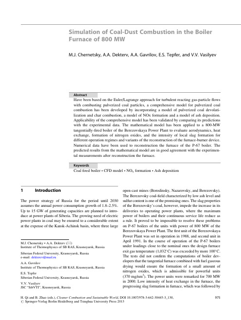
Simulation of Coal-Dust Combustion in the Boiler Furnace of800MWM.J.Chernetsky,A.A.Dekterv,A.A.Gavrilov,E.S.Tepfer,and V.V.Vasilyev AbstractHave been based on the Euler/Lagrange approach for turbulent reacting gas-particleflows with combusting pulverized coal particles,a comprehensive model for pulverized coal combustion has been developed by incorporating a model of pulverized coal devolati-lization and char combustion,a model of NOx formation and a model of ash deposition.Applicability of the comprehensive model has been validated by comparing its predictions with the experimental data.The mathematical model has been applied to a800-MW tangentially-fired boiler of the Berezovskaya Power Plant to evaluate aerodynamics,heat exchange,formation of nitrogen oxides,and the intensity of local slag formation for different operation regimes and variants of the reconstruction of the furnace-burner device.Numerical data have been used to reconstruction the furnace of the P-67boiler.The predicted results from the mathematical model are in good agreement with the experimen-tal measurements after reconstruction the furnace.KeywordsCoalfired boiler CFD model NO x formation Ash deposition1IntroductionThe power strategy of Russia for the period until2030 assumes the annual power consumption growth of1.8–2.5%. Up to15GW of generating capacities are planned to intro-duce at power plants of Siberia.The growing need of electric power plants in coal may be ensured to a considerable extent at the expense of the Kansk-Achinsk basin,where three large open-cast mines(Borodinsky,Nazarovsky,and Berezovsky). The Berezovsky coal-field characterized by low ash level and sulfur content is one of the promising ones.The slag properties of the Berezovsky’s coal,however,impede the increase in its deliveries to operating power plants,where the maximum power of boilers and their continuous service life reduce as a rule.It proved to be impossible to resolve these problems on P-67boilers of the units with power of800MW of the Berezovskaya Power Plant.Thefirst unit of the Berezovskaya Power Plant was set in operation in1988,and second unit in April1991.In the course of operation of the P-67boilers under loadings close to the nominal ones the design furnace exit gas temperature(1,032 C)was exceeded by more100 C. The tests did not confirm the computations of boiler dev-elopers that the tangential furnace combined with fuel gaseous drying would ensure the formation of a small amount of nitrogen oxides,which is admissible for powerful units (370mg/nm3).The power units were remarked for700MW in2000.Low intensity of heat exchange in the furnace,the progressing slag formation in furnace,which was followed byM.J.Chernetsky A.A.Dekterv(*)Institute of Thermophysics of SB RAS,Krasnoyarsk,RussiaSiberian Federal University,Krasnoyarsk,Russiae-mail:dekterev@mail.ruA.A.GavrilovInstitute of Thermophysics of SB RAS,Krasnoyarsk,RussiaE.S.TepferSiberian Federal University,Krasnoyarsk,RussiaV.V.VasilyevJSC“SibVTI”,Krasnoyarsk,RussiaH.Qi and B.Zhao(eds.),Cleaner Combustion and Sustainable World,DOI10.1007/978-3-642-30445-3_130,#Springer-Verlag Berlin Heidelberg and Tsinghua University Press2013975the growth of maximum gas temperatures before downtake gas ducts the formation of slag lumps.Local slagging of the cold hopper slopes resulted in closing of screws and urgent stops of boilers.At the execution of complex scientific and research,recon-struction,and setting-up works,the lot of tasks related to the intensity increase of heat exchange,decrease NO x in the furnace of the P-67boiler were solved during several recent years.One of the tasks was mathematical modelling of the aerodynamics,heat exchange,formation of nitrogen oxides, and local slagging intensity for various operation regimes and variants of the reconstruction of furnace/burner device.This work presents a comprehensive model for pulverized coal combustion in coalfired systems.This model was imple-mented in the in-house CFD code«s Flow».And in-house CFD code«s Flow»has been applied for the simulation of the furnace of the P-67boiler.2Mathematical ModelThe model of non-isothermal incompressible multi-component gas was assumed as a model offlow in combustion chamber. The gasflow in the studied problem is considered as esta-blished,thus all equations are written in the steady-state form.It is assumed that combustion gases consist of N2,O2, CO2,H2O and complex of volatiles VOL.The model includes the following equations:equation of continuity@r @t þr r vðÞ¼0;(1)equation of momentum balance@r v @t þr r vÁvðÞ¼Àr pþrðt mþt tÞþðrÀr1Þg(2)where the viscous stress tensor ist m ij¼mð@u i@x jþ@u j@x iÞÀ23d ij@u k@x k;t t is the Reynolds stress tensor;equation of i-th component concentration(mass fraction) transfer@r f i @t þr r vÁf iðÞ¼rðD iþm tSc iÞÁr f iþS i;(3)where D is the molecular diffusion constant,Sc–turbulentSchmidt number,S–source term describing reactions;equation of energy transfer@r h@tþr r vÁhðÞ¼rðlþc P m tPr tÞÁr TþS chþS R;(4)S ch,S R are source terms describing,correspondingly,energy effect of reactions and radiation heat transfer.The modified high-Reynolds k-e model of turbulence(Chen k-e model)is used to describe the turbulent charac-teristics offlow.The equations determining the kineticenergy of turbulence and its dissipation rate have a form[1]:@r k@tþr r vÁkðÞ¼rðmþm ts kÞÁr kþGÀre@re@tþr r vÁeðÞ¼rðmþm ts eÞÁr eþC1ekGÀC2re2kþC3G2r k(5)where G is the rate of turbulence generation:G¼t t ij@u i@x j;turbulent viscosity is determined asm t¼C m rk2e:Reynolds stress tensor has a formt t ij¼m tð@u i@x jþ@u j@x iÞÀ23d ij r kThe empirical constants C m¼0.09,s k¼0.8,s e¼1.15,С1¼1.15,C2¼1.9,C3¼0.25are given in the work[1].These constants are approved for a wide class of isothermalflows.The form of k-e model is adapted for fully developedturbulentflows.In the near-wall region wall function areused to save computational resources.Temperature of mixture T in each point offlowfield isfound using the known local values of enthalpy and mixturecomponents content:h¼X Nm¼1h mðTÞf m;976M.J.Chernetsky et al.where the dependencies of component enthalpy on tempera-ture h m(T)is described by polynomials of5th degree.Radi-ation is the dominant heat transfer mechanism.The modeling of radiant energy transfer is conducted basing on the P1approximation of spherical harmonics for a grey medium[2].The advantage of this method is easiness of its matching with methods of aerodynamics and heat transfer calculation realized in curvilinear meshes.The absorption coefficients were calculated using the weighted-sum-of-gray-gases model.Calculation of volatile fuel components combustion is based on the use of global irreversible reactions between fuel and oxidant.In this model the reaction rate is limited by the rate of turbulent mixing of fuel and oxidant.The reaction rate RVOL is determined in the model of“eddy break-up”[3]:R VOL¼ÀA rekmin f VOL;f O2S O2;(6)where A is an empirical constant equal4.0;f VOL,f O2are concentrations of volatiles and oxidant;S O2is the stoichio-metric coefficient in the combustion reaction.3Coal Dust CombustionThe Lagrange method was used in the present work to model of coal dust motion.During the modeling,the main forces acting on a particle were the force of phases inter-action(aerodynamic resistance force)and gravity force.As the coal particles moves,it is heated up and it undergoes a number of process:extraction of residual moisture and volatile components,combustion of volatile components and char.When the coal particle advances in the furnace,the reac-tion processes of vaporization,coal pyrolysis and char com-bustion are considered.The coal particle consists of four components:water,volatiles,carbon and ash.Vaporization of moisture from the coal particle is described by the diffusion-limited model.Coal pyrolysis is modelled by a simple,one-step mechanism and the volatile composition is assumed to be constant.The reaction rate of coal pyrolysis is taken from experimental data.Char combustion is controlled by the chemical surface reaction and the oxygen diffusion to the particle.This model includes the factor Z which describes the transition between the char combustion regime limited by the rate of oxygen diffusion and the regime is sufficiently limited by the chem-ical reaction rate.Char particles are considered to burn at constant density and variable size.The diameter change of a particle follows:d dd t¼2r kÃK C S(7)K C S¼b C O2ð273=T gÞÃa K(8)a K¼11a k:kin1a k:diffif a k:kin< a k:diff(9)a K¼a k:diff if a k:kin> a k:diff(10)a k:diff¼Nu D DdNu D¼2þ0:22Pe0:66a k:kin¼K K eÀE k=RTr k is the density of the char particle(kg m3);K C S is the char combustion rate(kg m–2*s–1);Nu D is the diffusion Nusselt number;D is the bulk molecular diffusion coefficient(m2/s);a k,kin is the reaction-rate coefficient for a chemical reaction (ms–1),a k,diff is the reaction-rate coefficient for diffusion (ms–1)The instantaneous burning rate of an individual parti-cle is determined from temperature,velocity,and size infor-mation by solving the energy balance for the particle, assuming a spherical,homogeneous,reacting particle surrounded by a chemically frozen boundary layer(i.e., single-film model).Heat losses from convection and radia-tion are considered,as well as the effects Stefanflow:m p C p4p r pd T pd t¼esðT4radÀT4pÞþa convðTÀT pÞþQH4p r p(11)a conv is the convection heat transfer coefficient:a conv¼Nu l2r pThe correction to the heat-transfer equation due to Stefan flow is provided modification of Nusselt number:Nu¼2þPe2À37960Pe2ÀPe Pe4ÀPe2where Pe is a Peclet number, Pe is a modified version of the Peclet number(i.e.,the ratio of the convective velocity of the net mass leaving the particle surface to the diffusive velocity of heat leaving the surface).Simulation of Coal-Dust Combustion in the Boiler Furnace of800MW977When char burn,heat losses from convection is much larger than that is predicted for not burning particles.In the model is used correlation coefficient Kcomb [4]:a comb conv ¼a conv K comb ;K comb ¼145eÀ5;000T;(12)a comb conv ;a conv -are convective heat transfer coefficients forburning and not burning coal particle respectively.The influence of particles on the averaged gas motion,the gas components concentration and enthalpy was taken into account on the base of PSI-cell method proposed by Crow [5].In the slagging models,the particle transport process was modeled using stochastic trajectory model.For particle sticking model,the particle sticking probability is primarily concerned with particle temperature.If the ash particle temperature is less than the critical ash particle temperature or the critical ash wall temperature,the particle sticking probability on the wall is 0;otherwise it is 1.The critical ash particle temperature follows:T slag ;cr ¼945þ40ÃCaO ðd Þ½ =SiO 2ðd ÞþFe 2O 3ðd Þ½ (13)Where CaO(d ),SiO 2(d ),Fe 2O 3(d )depend on the diame-ter of ash particle.Dependence of ash components of the Berezovo coal was taken from the experiment data.4NOx FormationIn the process of NOx formation simulation threemechanisms are taken into account:formation of thermal NOx according Zeldovich’s model [6],formation of prompt NOx according the Fenimore’s model [7]and formation of fuel NOx [8].Additional equations for NO and intermediate hydrogen cyanide HCN transfer are introduced:@r f NO@tþr r vf NO ðÞ¼r D r f NO ðÞþS NO @r f HCN@tþr r vf HCN ðÞ¼r D r f HCN ðÞþS HCN(14)The source term in the equation of NO transfer describing thermal mechanism [6]may be written asS thermal ÀNO x ¼M NOd NO ½ d twhere d[NO]/dt is calculated as following:d NO ½ d t ¼2O ½ k 1k 2O 2½ N 2½ Àk À1k À2NO ½2k 2O 2½ þk À1NO ½:(15)Assuming the partial equilibrium for oxygen atom density [O],we obtainO ½ ¼36:64T 1=2O 2½ 1=2exp À27123=T ðÞReaction rate constants (m 3/(mol s))are equalk 1¼1:8Á108exp À38;370=T ðÞk À1¼3:8Á107exp À425=T ðÞk 2¼1:8Á104ÁT Áexp À4;680=T ðÞk À2¼3:8Á103ÁT Áexp À20;820=T ðÞThe prompt NOx forms in the presence of hydrocarbon radicals which prevail in fuels with high molecular H:C rate.The mechanism of prompt NOx formation was described by [7].Source term in the equation of NO transfer may be writtenS prompt ÀNO x ¼M NOd NO ½d t;d[NO]/dt is calculated according the expression:d NO ½ d t ¼k pr O 2½ aN 2½ VOL ½ exp ÀE a RT;(16)wherek pr ¼1:2Á107RT =p ðÞa þ1E a ¼60kcal Âmol À1Oxygen reaction order are depends on flame conditions [9].The fuel NOx is a result of reaction between oxygen and fuel nitrogen.In the process of coal fuel gasification and char burn there takes place the transformation of nitrogen containing compounds to NH 3(ammonia)and HCN (hydro-gen cyanide).Depending on scheme of chemical reactions between these compounds and combustion gases,formation of NO or N 2takes place.Modified de Soete model [8],consisting of three global reactions,is realized to calculate the fuel NOx:d x HCNd t ¼À3:5Á1010exp ðÀ3;370=T Þx HCN x a O 2d x HCNd t ¼À3Á1012exp ðÀ30;200=T Þx HCN x NO d x NOd t¼À2:7Á106exp ðÀ9;466=T Þx NO x C n H m:(17)978M.J.Chernetsky et al.5Numerical MethodThe method of control volume on the structured curvilinear non-orthogonal meshes with multi block technique is used for the numerical implementation.For the pressure-velocity coupling,the SIMPLE–C algorithm is used.The high order scheme is applied for approximation of convective terms.Solving the algebraic equations sets is accomplished vie effective procedures based on variation method of incom-plete factorization.6Results and DiscussionThe coal-fired boiler P-67of Berezovskaya has a T-shape assembling (Fig.1).Furnace with square section 23.08Â23.08m has height 60m from the center ofhopper to the bottom of plates.32direct flow burners are allocated in four stories and directed clockwise and tangen-tially to an imaginary circle with diameter 2.3m.Axes of burners are inclined at angle of 10to the horizontal plane.The fuel element composition is given in Table 1.Numerical results for base variant are presented Fig.2.The configuration and works parameters of base variant were taken according to the furnace before reconstruction in 2004.The calculation results were compared with the experimental data.The aerodynamic structure of gas flows in the furnace is shown on Fig.2a .The flame impingementisFig.1Coal-fired boiler on Beryozovskaya Power PlantTable 1Coal propertiesProximate and ultimate analysis (%)W rA d C r H r S r N r O r V daf 34.7 6.9144.02 2.980.240.5213.0346.9Combustion heat (kcal/kg):Q i r¼3,750Simulation of Coal-Dust Combustion in the Boiler Furnace of 800MW 979observed in upper part of the cold hopper and between the burner rows with a temperature growth in the near-wall zone.The modeling has shown that the regions of intensive slagging near even blocks of burners are caused by the aero-dynamic structure offlow(Fig.2b).In the region between stories of burners there occurs the formation of corner vor-texes with directflow throwing on the walls which is clearly displayed by the both temperaturefield character(Fig.2c) and sedimentation development(Fig.4a).The maximum gas temperatures within the furnace are 1,400 C by the calculations.The furnace exit temperature is1,116and1,220 C by numerical result and experiment, respectively.Concentration NO x is460mg/nm3(experi-ment’s temperature is450mg/nm3).Slag fall into the cold hopper is637kg/h by thecalculations,and639kg/h by experiment.As it can be seen,the comprehensive model provides reasonable agree-ment with the experimental data(Fig.3).Numerical investigations of the following possible variants of reconstruction were carried out:anization of bottom blowing;2.Concentric combustion(over air blowing in the burnersplane,32nozzles);bination of bottom blowing and concentric combus-tion(8nozzles at two upper stories of odd blocks of burners);anization of air nozzles storey above the active com-bustion zone;bination of nozzles in upper burners stories(concen-tric combustion)and vertical stage of nozzles;anization of two air nozzles stories above the activecombustion zone.The main attention was paid to a correct specification of boundary conditions,optimal combination of the model computation and full-scale experiment.The results of ther-mal and hydraulic computations of the boiler adapted to the base experience.Thermal resistance of the layer of outer deposits was determined at the mathematical model adapta-tion to the base experience on furnace exit gas temperature.A comparative analysis of computed variants of recon-struction was performed according to such criteria as the flame impingement intensity(the maximum velocity of gases along a normal to the wall),the intensity of particles separation on the walls,theflame maximum temperature,the maximum volume and near-wall temperatures of gases,the furnace exit temperature and its non-uniformity,the imping-ing heatfluxes,the burnout,the concentration ofnitrogen Fig.2Flow in the existing furnace:(a)vertical section through center;(b)horizontal section between stories of burners;(c)temperaturefield in near-wall region980M.J.Chernetsky et al.oxides,the variation of a deposition in the cold hopper.Any of the reconstruction options considered would result in the decrease of gases temperatures in near-wall zone of active combustion area and in hopper.Respectively,the slagging rate must decrease.Maximal effect as related to the existing variant is reached via combining bottom blowing and concentric com-bustion.The dynamics of wall slagging in the existing and recommended variant is presented on Fig.4.Comparison of calculated variants by the mean tempera-ture at the outlet of furnace has shown a decrease of temper-ature in the variant with bottom blowing and concentric combustion as compared with the existing variant (Fig.5),here the level of NO x ejection didn’t exceed the normative requirements (Fig.6).Variant of furnace reconstruction with loading of lower burner rows (the fourth row is used for air blowing only)fuel coarsening,lower hot blowing (air rate is 7%)was chosen by numerical investigation.For the first and second units of the Berezovskaya Power Plant was done reconstruction.In the reconstruction were used numerical results.In the course of operation of the P-67boiler under loadings close to the nominal ones (800MW)was shown operation of the boiler over a long period of time after reconstruction.Figure 7shows the temperature of gas along the furnace after reconstruction.Concentration NO x was 409mg/nm 3by experiment.Coefficient of efficiency was91.3%.Fig.3Temperature ( C)along thefurnaceFig.4Zones of intensive slagging.(a )Existing variant;(b )Variant with bottom blowing and concentric combustion1020103010401050106010701080109011001110base 123456Fig.5The average gas temperature at the furnace outlet, C for different variantsbase123456Fig.6NO x ejection level,mg/nm 3Simulation of Coal-Dust Combustion in the Boiler Furnace of 800MW9817Conclusion1.The mathematical model of coal combustion in the a pulverized coal-fired boiler P-67has been developed on the basis of in-house CFD code «s Flow »for the pur-pose of calculation of 3D turbulent gas flows,heat and mass transfer,convective and radiation heat exchange taking into account the processes of particles drying,pyrolysis,char combustion,NO x emission and ash deposition.2.Numerical investigations of the possible variants of recon-struction furnace were carried anization of bottom blowing,the concentric combustion,the air nozzles storeyabove the active combustion zone and combination variants was considered.3.Variant of furnace reconstruction with loading of lower burner rows (the fourth row is used for air blowing only)fuel coarsening,lower hot blowing (air rate is 7%)was chosen by numerical investigation.The predicted results from the mathematical model are in good agreement with the experimental measurements after reconstruc-tion the furnace.The results of tests after reconstruction enabled to remove the limitations for the boiler slag-free power.References1.Chen YS,Kim putation of turbulent flows using an extended k-e _turbulence closure model.NASA CR-179204;1987.2.Siegel R,Howell JR.Thermal radiation heat transfer.Washington,DC:Hemisphere Publishing Corporation;1992.3.Magnussen BF,Hjertager BW.On the structure of turbulence and a generalised eddy dissipation concept for chemical reaction in turbu-lent flow.In:19th AIAA Aerospace Meeting;St.Louis,MO;1981.4.Babiy VI,Kuvaev YF.Pulverized coal particles combustion and calculation of coal-dust flame.Moscow:Energoatomizdat;1986.5.Crow CT,Sharma MP,Stock DE.The particle source in cell (PSI-CELL)model for gas-droplet flows.J Fluids Eng Trans ASME.1977;99:325–32.6.Zeldovich YB.The oxidation of nitrogen in combustion and explosions.Acta Physicochim USSR.1946;21:577.7.Fenimore CP.Studies of fuel-nitrogen in rich flame gases.In:17th Symposium (International)Combustion.Pittsburgh:The Combus-tion Institute;1979.p.661.8.Magel HC,Greul U,Schnell U,Spliethoff H,Hein KRG.NOx-reduction with staged combustion –comparison of experimental and modeling results.In:Proceedings Joint Meeting of the Portu-guese,British,Madeira:Spanish and Swedish Section of the Com-bustion Institute;1996.9.De Soete GG.Overall reaction rates of NO and N N 2formation from fuel nitrogen.In:15th Symposium (International)on Combustion.Pittsburgh:The Combustion Institute;1975.p.1093.Fig.7Temperature ( C)along the furnace982M.J.Chernetsky et al.。
黑带doe试题

2.DOE 实验设计及分析的主要步骤和内容 (7 分) 答案: 1)明确实验目的 2)选择输出变量 3)决定因子和水平 4)选择 DOE 类型 5)实施实验并收集数据 6)分析实验结果 7)得出实 验结论和 改善方 案
验策略; E)不管实验策略,只是获得实验数据并决定下一步该做什么。
1. DOE 中的随机化是利用实验次序的随机消除可能与实验次序有关的某些因素对实验结果 的影响。 ( OK ) 2.DOE 中的模块化是利用高次交互作用的稀疏性原理,把可能对实验结果造成影响的外部因素 进行模块化处理,让它与高次交互作用而不是低次或主效果混淆。 ( OK ) 3.如果有可能的话,通常在最终实验设计中要构造一些重复。 ( OK ) 4.实验设计中的模块化(Block)只能选择 2 水平。 ( NG ) 5. 残差检验的目的是验证统计分析的结论是否完全及正确,是否有遗漏的因子或得出的方程式 是否是最佳的。 ( OK ) 6.部分 阶乘法 的原理 也是根 据交互 作用的 稀疏性 原理,在实验 不能保 证全部 进行的 情况下 ,以 高次作用相互混淆为代价,即减少了实验次数有不影响主效果分析的方法。 ( OK ) 7.多重回归中的 Stat> Regression>Stepwise 功能能够给出不同因子的组合回归模型所能解释描 述部分占总变动的多少。 ( OK ) 8.在表面反映法中,垂直于等高线的法线方向是以最快的速度找到全局最佳 点的方向。 ( OK ) 9.如果发现在改善过程中通过改善很难达到项目的目标,可能需要按照六西格玛设计 (DFSS) 的原理,重新设计产品或服务流程。 ( OK ) 10.在对 利益相 关者的 分析中 ,只要 你有相 对的权 力,就 可以利 用惩罚 的手段 使对方 改变自 己的 观点或立场,要求他支持你的工作。 ( NG ) 11.人 的失误 是难免 的, 设备也 会发生 故障, 因此 零缺陷 只能是 一个理 想目标 ,是 可望而 不可 及的。 ( NG ) 12.有无标准、标准是否合适与是否遵守标准称为标准的三大原则。 ( OK ) 13.控制计划只适用于制造类的项目,对库存、服务等职能部门的项目不适用。 ( NG ) 14.SPC 控制图的原始目的是通过统计数据找出其上下控制线,所以项目完成后只要对相关过 程的输入或输出进行控制线的计算即可。 ( NG ) 15.个体 图的基 本假设 是独立 和正态 ,如果 不是正 态的数 据一 定要转 换成正 态才可 以画个 体图。 ( OK )
基于差分进化优化随机森林模型的油层结垢预测方法
基于差分进化优化随机森林模型的油层结垢预测方法下载提示:该文档是本店铺精心编制而成的,希望大家下载后,能够帮助大家解决实际问题。
文档下载后可定制修改,请根据实际需要进行调整和使用,谢谢!本店铺为大家提供各种类型的实用资料,如教育随笔、日记赏析、句子摘抄、古诗大全、经典美文、话题作文、工作总结、词语解析、文案摘录、其他资料等等,想了解不同资料格式和写法,敬请关注!Download tips: This document is carefully compiled by this editor. I hope that after you download it, it can help you solve practical problems. The document can be customized and modified after downloading, please adjust and use it according to actual needs, thank you! In addition, this shop provides you with various types of practical materials, such as educational essays, diary appreciation, sentence excerpts, ancient poems, classic articles, topic composition, work summary, word parsing, copy excerpts, other materials and so on, want to know different data formats and writing methods, please pay attention!基于差分进化优化随机森林模型的油层结垢预测方法摘要本文针对油田开发中的结垢问题,提出了一种基于差分进化优化的随机森林模型,用于预测油层结垢的发生和发展情况。
Focused information criterion and model averaging for generalized
The Annals of Statistics2011,V ol.39,No.1,174–200DOI:10.1214/10-AOS832©Institute of Mathematical Statistics,2011FOCUSED INFORMATION CRITERION AND MODEL A VERAGING FOR GENERALIZED ADDITIVE PARTIAL LINEAR MODELSB Y X INYU Z HANG1AND H UA L IANG2Chinese Academy of Sciences and University of RochesterWe study model selection and model averaging in generalized additive partial linear models(GAPLMs).Polynomial spline is used to approximatenonparametric functions.The corresponding estimators of the linear para-meters are shown to be asymptotically normal.We then develop a focusedinformation criterion(FIC)and a frequentist model average(FMA)estimatoron the basis of the quasi-likelihood principle and examine theoretical proper-ties of the FIC and FMA.The major advantages of the proposed proceduresover the existing ones are their computational expediency and theoretical re-liability.Simulation experiments have provided evidence of the superiority ofthe proposed procedures.The approach is further applied to a real-world dataexample.1.Introduction.Generalized additive models,which are a generalization of the generalized models and involve a summand of one-dimensional nonparamet-ric functions instead of a summand of linear components,have been widely used to explore the complicated relationships between a response to treatment and pre-dictors of interest[Hastie and Tibshirani(1990)].Various attempts are still being made to balance the interpretation of generalized linear models and theflexibility of generalized additive models such as generalized additive partial linear models (GAPLMs),in which some of the additive component functions are linear,while the remaining ones are modeled nonparametrically[Härdle et al.(2004a,2004b)].A special case of a GAPLM with a single nonparametric component,the gener-alized partial linear model(GPLM),has been well studied in the literature;see, for example,Severini and Staniswalis(1994),Lin and Carroll(2001),Hunsberger (1994),Hunsberger et al.(2002)and Liang(2008).The profile quasi-likelihood procedure has generally been used,that is,the estimation of GPLM is made com-putationally feasible by the idea that estimates of the parameters can be found for a known nonparametric function,and an estimate of the nonparametric function can Received February2010;revised May2010.1Supported in part by the National Natural Science Foundation of China Grants70625004and 70933003.2Supported in part by NSF Grant DMS-08-06097.AMS2000subject classifications.Primary62G08;secondary62G20,62G99.Key words and phrases.Additive models,backfitting,focus parameter,generalized partially lin-ear models,marginal integration,model average,model selection,polynomial spline,shrinkage methods.174GENERALIZED ADDITIVE PARTIALLY LINEAR MODELS175 be found for the estimated parameters.Severini and Staniswalis(1994)showed that the resulting estimators of the parameter are asymptotically normal and that estimators of the nonparametric functions are consistent in supremum norm.The computational algorithm involves searching for maxima of global and local likeli-hoods simultaneously.It is worthwhile to point out that studying GPLM is easier than studying GAPLMs,partly because there is only one nonparametric term in GPLM.Correspondingly,implementation of the estimation for GPLM is simpler than for GAPLMs.Nevertheless,the GAPLMs are moreflexible and useful than GPLM because the former allow several nonparametric terms for some covariates and parametric terms for others,and thus it is possible to explore more complex re-lationships between the response variables and covariates.For example,Shiboski (1998)used a GAPLM to study AIDS clinical trial data and Müller and Rönz (2000)used a GAPLM to carry out credit scoring.However,few theoretical re-sults are available for GAPLMs,due to their generalflexibility.In this article,we shall study estimation of GAPLMs using polynomial spline,establish asymptotic normality for the estimators of the linear parameters and develop a focused in-formation criterion(FIC)for model selection and a frequentist model averaging (FMA)procedure in construction of the confidence intervals for the focus parame-ters with improved coverage probability.We know that traditional model selection methods such as the Akaike informa-tion criterion[AIC,Akaike(1973)]and the Bayesian information criterion[BIC, Schwarz(1978)]aim to select a model with good overall properties,but the se-lected model is not necessarily good for estimating a specific parameter under consideration,which may be a function of the model parameters;see an inspiring example in Section4.4of Claeskens and Hjort(2003).Exploring the data set from the Wisconsin epidemiologic study of diabetic retinopathy,Claeskens,Croux and van Kerckhoven(2006)also noted that different models are suitable for different patient groups.This occurrence has been confirmed by Hand and Vinciotti(2003) and Hansen(2005).Motivated by this concern,Claeskens and Hjort(2003)pro-posed a new model selection criterion,FIC,which is an unbiased estimate of the limiting risk for the limit distribution of an estimator of the focus parameter,and systematically developed a general asymptotic theory for the proposed criterion. More recently,FIC has been studied in several models.Hjort and Claeskens(2006) developed the FIC for the Cox hazard regression model and applied it to a study of skin cancer;Claeskens,Croux and van Kerckhoven(2007)introduced the FIC for autoregressive models and used it to predict the net number of new personal life insurance policies for a large insurance company.The existing model selection methods may arrive at a model which is thought to be able to capture the main information of the data,and to be decided in advance in data analysis.Such an approach may lead to the ignoring of uncertainty intro-duced by model selection.Thus,the reported confidence intervals are too narrow or shift away from the correct location,and the corresponding coverage probabili-ties of the resulting confidence intervals can substantially deviate from the nominal176X.ZHANG AND H.LIANGlevel[Danilov and Magnus(2004)and Shen,Huang and Ye(2004)].Model aver-aging,as an alternative to model selection,not only provides a kind of insurance against selecting a very poor model,but can also avoid model selection instability [Yang(2001)and Leung and Barron(2006)]by weighting/smoothing estimators across several models,instead of relying entirely on a single model selected by some model selection criterion.As a consequence,analysis of the distribution of model averaging estimators can improve coverage probabilities.This strategy has been adopted and studied in the literature,for example,Draper(1995),Buckland, Burnham and Augustin(1997),Burnham and Anderson(2002),Danilov and Mag-nus(2004)and Leeb and Pöstcher(2006).A seminal work,Hjort and Claeskens (2003),developed asymptotic distribution theories for estimation and inference af-ter model selection and model averaging across parametric models.See Claeskens and Hjort(2008)for a comprehensive survey on FIC and model averaging.FIC and FMA have been well studied for parametric models.However,few ef-forts have been made to study FIC and FMA for semiparametric models.To the best of our knowledge,only Claeskens and Carroll(2007)studied FMA in semi-parametric partial linear models with a univariate nonparametric component.The existing results are hard to extend directly to GAPLMs,for the following reasons: (i)there exist nonparametric components in GAPLMs,so the ordinary likelihood method cannot be directly used in estimation for GAPLMs;(ii)unlike the semi-parametric partial linear models in Claeskens and Carroll(2007),GAPLMs allow for multivariate covariate consideration in nonparametric components and also al-low for the mean of the response variable to be connected to the covariates by a link function,which means that the binary/count response variable can be consid-ered in the model.Thus,to develop FIC and FMA procedures for GAPLMs and to establish asymptotic properties for these procedures are by no means straightfor-ward to achieve.Aiming at these two goals,wefirst need to appropriately estimate the coefficients of the parametric components(hereafter,we call these coefficients “linear parameters”).There are two commonly used estimation approaches for GAPLMs:thefirst is local scoring backfitting,proposed by Buja,Hastie and Tibshirani(1989);the second is an application of the marginal integration approach on the nonparamet-ric component[Linton and Nielsen(1995)].However,theoretical properties of the former are not well understood since it is only defined implicitly as the limit of a complicated iterative algorithm,while the latter suffers from the curse of dimen-sionality[Härdle et al.(2004a)],which may lead to an increase in the computa-tional burden and which also conflicts with the purpose of using a GAPLM,that is,dimension reduction.Therefore,in this article,we apply polynomial spline to approximate nonparametric functions in GAPLMs.After the spline basis is cho-sen,the nonparametric components are replaced by a linear combination of spline basis,then the coefficients can be estimated by an efficient one-step maximizing procedure.Since the polynomial-spline-based method solves much smaller sys-tems of equations than kernel-based methods that solve larger systems(which mayGENERALIZED ADDITIVE PARTIALLY LINEAR MODELS177 lead to identifiability problems),our polynomial-spline-based procedures can sub-stantially reduce the computational burden.See a similar discussion about this computational issue in Yu,Park and Mammen(2008),in the generalized additive models context.The use of polynomial spline in generalized nonparametric models can be traced back to Stone(1986),where the rate of convergence of the polynomial spline es-timates for the generalized additive model werefirst obtained.Stone(1994)and Huang(1998)investigated the polynomial spline estimation for the generalized functional ANOV A model.In a widely discussed paper,Stone et al.(1997)pre-sented a completely theoretical setting of polynomial spline approximation,with applications to a wide array of statistical problems,ranging from least-squares re-gression,density and conditional density estimation,and generalized regression such as logistic and Poisson regression,to polychotomous regression and hazard regression.Recently,Xue and Yang(2006)studied estimation in the additive coef-ficient model with continuous response using polynomial spline to approximate the coefficient functions.Sun,Kopciuk and Lu(2008)used polynomial spline in par-tially linear single-index proportional hazards regression models.Fan,Feng and Song(2009)applied polynomial spline to develop nonparametric independence screening in sparse ultra-high-dimensional additive models.Few attempts have been made to study polynomial spline for GAPLMs,due to the extreme technical difficulties involved.The remainder of this article is organized as follows.Section2sets out the model framework and provides the polynomial spline estimation and asymptotic normality of estimators.Section3introduces the FIC and FMA procedures and constructs confidence intervals for the focus parameters on a basis of FMA esti-mators.A simulation study and real-world data analysis are presented in Sections 4and5,respectively.Regularity conditions and technical proofs are presented in the Appendix.2.Model framework and estimation.We consider a GAPLM where the response Y is related to covariates X=(X1,...,X p)T∈R p and Z=(Z1,..., Z d)T∈R d.Let the unknown mean response u(x,z)=E(Y|X=x,Z=z)and the conditional variance function be defined by a known positive function V, var(Y|X=x,Z=z)=V{u(x,z)}.In this article,the mean function u is defined via a known link function g by an additive linear functiong{u(x,z)}=pα=1ηα(xα)+z Tβ,(2.1)where xαis theαth element of x,βis a d-dimensional regression parameter and theηα’s are unknown smooth functions.To ensure identifiability,we assume that E{ηα(Xα)}=0for1≤α≤p.Letβ=(βT c,βT u)T be a vector with d=d c+d u components,whereβc con-sists of thefirst d c parameters ofβ(which we certainly wish to be in the selected178X.ZHANG AND H.LIANGmodel)and βu consists of the remaining d u parameters (for which we are unsure whether or not they should be included in the selected model).In what follows,we call the elements of z corresponding to βc and βu the certain and exploratory vari-ables,respectively.As in the literature on FIC,we consider a local misspecification framework where the true value of the parameter vector βis β0=(βT c,0,δT /√n)T ,with δbeing a d u ×1vector;that is,the true model is away from the deduced model with a distance O(1/√n).This framework indicates that squared model biases and estimator variances are both of size O(1/n),the most possible large-sample approximations.Some arguments related to this framework appear in Hjort and Claeskens (2003,2006).Denote by βS =(βT c ,βT u,S )T the parameter vector in the S th submodel,in the same sense as β,with βu,S being a d u,S -subvector of βu .Let πS be the projec-tion matrix of size d u,S ×d u mapping βu to βu,S .With d u exploratory covariates,our setup allows 2d u extended models to choose among.However,it is not nec-essary to deal with all 2d u possible models and one is free to consider only a few relevant submodels (unnecessarily nested or ordered)to be used in the model se-lection or averaging.A special example is the James–Stein-type estimator studied by Kim and White (2001),which is a weighted summand of the estimators based on the reduced model (d u,S =0)and the full model (d u,S =d u ).So,the covariates in the S th submodel are X and S Z ,where S =diag (I d c ,πS ).To save space,we generally ignore the dimensions of zero vectors/matrices and identity matrices,simply denoting them by 0and I,respectively.If necessary,we will write their dimensions explicitly.In the remainder of this section,we shall investigate poly-nomial spline estimation for (βT c,0,0)based on the S th submodel and establish a theoretical property for the resulting estimators.Let η0= p α=1η0,α(x α)be the true additive function and the covariate X αbe distributed on a compact interval [a α,b α].Without loss of generality,we take all intervals [a α,b α]=[0,1]for α=1,...,p .Noting (A.7)in Appendix A.2,under some smoothness assumptions in Appendix A.1,η0can be well approximated by spline functions.Let S n be the space of polynomial splines on [0,1]of degree ≥1.We introduce a knot sequence with J interior knots,k − =···=k −1=k 0=0<k 1<···<k J <1=k J +1=···=k J + +1,where J ≡J n increases when sample size n increases and the precise order is given in condition (C6).Then,S n consists of functions ςsatisfying the following:(i)ςis a polynomial of degree on each of the subintervals [k j ,k j +1),j =0,...,J n −1,and the last subinterval is [k J n ,1];(ii)for ≥2,ςis ( −1)-times continuously differentiable on [0,1].For simplicity of proof,equally spaced knots are used.Let h =1/(J n +1)be the distance between two consecutive knots.Let (Y i ,X i ,Z i ),i =1,...,n ,be independent copies of (Y,X ,Z ).In the S th submodel,we consider the additive spline estimates of η0based on the independent random sample (Y i ,X i , S Z i ),i =1,...,n .Let G n be the collection of functionsGENERALIZED ADDITIVE PARTIALLY LINEAR MODELS179ηwith the additive formη(x)= pα=1ηα(xα),where each component functionηα∈S n.We would like tofind a functionη∈G n and a value ofβS that maximize the quasi-likelihood functionL(η,βS)=1nni=1Q[g−1{η(X i)+( S Z i)TβS},Y i],η∈G n,(2.2)where Q(m,y)is the quasi-likelihood function satisfying∂Q(m,y)∂m =y−mV(m).For theαth covariate xα,let b j,α(xα)be the B-spline basis function of de-gree .For anyη∈G n,one can writeη(x)=γT b(x),where b(x)={b j,α(xα),j=− ,...,J n,α=1,...,p}T are the spline basis functions andγ={γj,α,j=− ,...,J n,α=1,...,p}T is the spline coefficient vector.Thus,the maximiza-tion problem in(2.2)is equivalent tofinding values ofβ∗S andγ∗that maximize1 nni=1Q[g−1{γ∗T b(X i)+( S Z i)Tβ∗S},Y i].(2.3)We denote the maximizers as β∗S and γ∗S={ γ∗S,j,α,j=− ,...,J n,α=1,..., p}T.The spline estimator ofη0is then η∗S= γ∗T S b(x)and the centered spline esti-mators of each component function areη∗S,α(xα)=J nj=−γ∗S,j,αb j,α(xα)−1nni=1J nj=−γ∗S,j,αb j,α(X iα),α=1,...,p.The above estimation approach can be easily implemented with commonly used statistical software since the resulting model is a generalized linear model.For any measurable functionsϕ1,ϕ2on[0,1]p,define the empirical inner prod-uct and the corresponding norm asϕ1,ϕ2 n=n−1ni=1{ϕ1(X i)ϕ2(X i)}, ϕ 2n=n−1ni=1ϕ2(X i).Ifϕ1andϕ2are L2-integrable,define the theoretical inner product and the corre-sponding norm as ϕ1,ϕ2 =E{ϕ1(X)ϕ2(X)}, ϕ 22=Eϕ2(X),respectively.Let ϕ 2nαand ϕ 22αbe the empirical and theoretical norms,respectively,of a func-tionϕon[0,1],that is,ϕ 2nα=n−1ni=1ϕ2(X iα), ϕ 22α=Eϕ2(Xα)=1ϕ2(xα)fα(xα)dxα,where fα(xα)is the density function of Xα.180X.ZHANG AND H.LIANGDefine the centered version spline basis for anyα=1,...,p and j=− + 1,...,J n,b∗j,α(xα)=b j,α(xα)− b j,α 2α/ b j−1,α 2αb j−1,α(xα),with the stan-dardized version given byB j,α(xα)=b∗j,α(xα) b∗j,α 2α.(2.4)Note that tofind(γ∗,β∗S)that maximizes(2.3)is mathematically equivalent to finding(γ,βS)that maximizes(γ,βS)=1nni=1Q[g−1{γT B(X i)+( S Z i)TβS},Y i],(2.5)where B(x)={B j,α(xα),j=− +1,...,J n,α=1,...,p}T.Similarly to β∗S, γ∗S, η∗S and η∗S,α,we can define βS, γS, ηS and the centered spline estima-tors of each component function ηS,α(xα).In practice,the basis{b j,α(xα),j=− ,...,J n,α=1,...,p}T is used for data analytic implementation and the math-ematically equivalent expression(2.4)is convenient for asymptotic derivation.Letρl(m)={dg−1(m)dm }l/V{g−1(m)},l=1,2.Write T=(X T,Z T)T,m0(T)=η0(X)+Z Tβ0andε=Y−g−1{m0(T)}.T i,m0(T i)andεi are defined in the same way after replacing X,Z and T by X i,Z i and T i,respectively.Write(x)=E[Zρ1{m0(T)}|X=x]E[ρ1{m0(T)}|X=x],ψ(T)=Z− (X),G n=1√nni=1εiρ1{m0(T i)}ψ(T i),D=E[ρ1{m0(T)}ψ(T){ψ(T)}T]and =E[ρ21{m0(T)}ε2ψ(T){ψ(T)}T].The following theorem shows that the estimators βS on the basis of the S th submodel are asymptotically normal.T HEOREM1.Under the local misspecification framework and conditions (C1)–(C11)in the Appendix,√n{ βS−(βT c,0,0)T}=−( S D T S)−1 S G n+( S D T S)−1 S Dδ+o p(1)d−→−( S D T S)−1 S G+( S D T S)−1 S D0δwith G n d−→G∼N(0, ),where“d−→”denotes convergence in distribution.GENERALIZED ADDITIVE PARTIALLY LINEAR MODELS181 R EMARK1.If the link function g is identical and there is only one nonpara-metric component(i.e.,p=1),then the result of Theorem1will simplify to those of Theorems3.1–3.4of Claeskens and Carroll(2007)under the corresponding submodels.R EMARK2.Assume that d u=0.Theorem1indicates that the polynomial-spline-based estimators of the linear parameters are asymptotically normal.This is thefirst explicitly theoretical result on asymptotic normality for estimation of the linear parameters in GAPLMs and is of independent interest and importance. This theorem also indicates that although there are several nonparametric functions and their polynomial approximation deduces biases for the estimators of each non-parametric component,these biases do not make the estimators ofβbiased under condition(C6)imposed on the number of knots.3.Focused information criterion and frequentist model averaging.In this section,based on the asymptotic result in Section2,we develop an FIC model se-lection for GAPLMs,an FMA estimator,and propose a proper confidence interval for the focus parameters.3.1.Focused information criterion.Letμ0=μ(β0)=μ(βc,0,δ/√n)be afocus parameter.Assume that the partial derivatives ofμ(β0)are continuous in a neighborhood ofβc,0.Note that,in the S th submodel,μ0can be estimated by μS=μ([I d c,0d c×d u] T S βS,[0d u×d c,I d u] T S βS).We now show the asymptoticnormality of μS.Write R S= T S( S D T S)−1 S,μc=∂μ(βc,βu)∂βc |βc=βc,0,βu=0,μu=∂μ(βc,βu)∂βu |βc=βc,0,βu=0andμβ=(μT c,μT u)T.T HEOREM2.Under the local misspecification framework and conditions (C1)–(C11)in the Appendix,we have√n( μS−μ0)=−μTβR S G n+μTβ(R S D−I)δ+o p(1)d−→ S≡−μTβR S G+μTβ(R S D−I)0δ.Recall G∼N(0, ).A direct calculation yieldsE( 2S)=μTβR S R S+(R S D−I)δδT(R S D−I)Tμβ.(3.1)Let δbe the estimator ofδby the full model.Then,from Theorem1,we know thatδ=−[0,I]D−1Gn+δ+o p(1).182X.ZHANG AND H.LIANGIf we define =−[0,I ]D −1G +δ∼N(δ,[0,I ]D −1 D −1[0,I ]T ),then δd −→ .Following Claeskens and Hjort (2003)and (3.1),we define the FIC of the S thsubmodel asFIC S =μT β R S R S +(R S D −I ) 0 δ 0 δT (R S D −I )T (3.2)−(R S D −I ) 000I d u D −1 D −1 000I d u(R S D −I )T μβ,which is an approximately unbiased estimator of the mean squared error when √nμ0is estimated by √n μS .This FIC can be used for choosing a proper sub-model relying on the parameter of interest.3.2.Frequentist model averaging .As mentioned previously,an average esti-mator is an alternative to a model selection estimator.There are at least two advan-tages to the use of an average estimator.First,an average estimator often reduces mean square error in estimation because it avoids ignoring useful information from the form of the relationship between response and covariates and it provides a kind of insurance against selecting a very poor submodel.Second,model averaging pro-cedures can be more stable than model selection,for which small changes in the data often lead to a significant change in model choice.Similar discussions of this issue appear in Bates and Granger (1969)and Leung and Barron (2006).By choosing a submodel with the minimum value of FIC,the FIC estimators ofμcan be written as μFIC = S I (FIC selects the S th submodel) μS ,where I (·),an indicator function,can be thought of as a weight function depending on the dataviaδ,yet it just takes value either 0or 1.To smooth estimators across submodels,we may formulate the model average estimator of μasμ=S w(S | δ) μS ,(3.3)where the weights w(S |δ)take values in the interval [0,1]and their sum equals 1.It is readily seen that smoothed AIC,BIC and FIC estimators investigated in Hjort and Claeskens (2003)and Claeskens and Carroll (2007)share this form.The fol-lowing theorem shows an asymptotic property for the general model average esti-mators μdefined in (3.3)under certain conditions.T HEOREM 3.Under the local misspecification framework and conditions (C1)–(C11)in the Appendix ,if the weight functions have at most a countable num-ber of discontinuities ,then √n( μ−μ0)=−μT βD −1G n +μT β Q( δ) 0 δ − 0 δ+o p (1)d −→ ≡−μT βD −1G +μT β Q( ) 0 − 0 ,GENERALIZED ADDITIVE PARTIALLY LINEAR MODELS183where Q(·)=Sw(s|·)R S D and is defined in Section3.1.Referring to the above theorems,we construct a confidence interval forμbased on the model average estimatorˆμ,as follows.Assume that κ2is a consistent esti-mator ofμTβD−1 D−1μβ.It is easily seen that√n( μ−μ0)−μTβQ( δ)δ−δκd−→N(0,1).If we define the lower bound(low n)and upper bound(up n)byμ−μTβQ( δ)δ−δ√n∓z j κ/√n,(3.4)where z j is the j th standard normal quantile,then we have Pr{μ0∈(low n,up n)}→2 (z j)−1,where (·)is a standard normal distribution function.Therefore,the interval(low n,up n)can be used as a confidence interval forμ0with asymptotic level2 (z j)−1.R EMARK3.Note that the limit distribution of √n( μ−μ0)is a nonlinearmixture of several normal variables.As argued in Hjort and Claeskens(2006),a direct construction of a confidence interval based on Theorem3may not be easy. The confidence interval based on(3.4)is better in terms of coverage probability and computational simplicity,as promoted in Hjort and Claeskens(2003)and ad-vocated by Claeskens and Carroll(2007).R EMARK4.A referee has asked whether the focus parameter can depend on the nonparametric functionη0.Our answer is“yes.”For instance,we consider a general focus parameter,η0(x)+μ0,a summand ofμ0,which we have studied,and a nonparametric value at x.We may continue to get an estimator ofη0(x)+μ0by minimizing(3.2)and then model-averaging estimators by weighting the estimators ofμ0andη0as in(3.3).However,the underlying FMA estimators are not root-n consistent because the bias of these estimators is proportional to the bias of the estimators ofη0,which is larger than n−1/2,whereas we can establish their rates of convergence using easier arguments than those employed in the proof of Theorem3.Even though the focus parameters generally depend onμ0andη0 of form H(μ0,η0)for a given function H(·,·),the proposed method can be still applied.However,to develop asymptotic properties for the corresponding FMA estimators depends on the form of H(·,·)and will require further investigation. We omit the details.Our numerical studies below follow these proposals when the focus parameters are related to the nonparametric functions.184X.ZHANG AND H.LIANG4.Simulation study.We generated 1000data sets consisting of n =200and 400observations from the GAPLMlogit {Pr (Y i =1)}=η1(X i,1)+η2(X i,2)+Z T i β=sin (2πX i,1)+5X 4i,2+3X 2i,2−2+Z Ti β,i =1,...,n,where:the true parameter β={1.5,2,r 0(2,1,3)/√n }T ;X i,1and X i,2are inde-pendently uniformly distributed on [0,1];Z i,1,...,Z i,5are normally distributed with mean 0and variance 1;when 1= 2,the correlation between Z i, 1and Z i, 2is | 1− 2|with =0or =0.5;Z i is independent of X i,1and X i,2.We set the first two components of βto be in all submodels.The other three may or may not be present,so we have 23=8submodels to be selected or av-eraged across.r 0varies from 1or 4to 7.Our focus parameters are (i)μ1=β1,(ii)μ2=β2,(iii)μ3=0.75β1+0.05β2−0.3β3+0.1β4−0.06β5and (iv)μ4=η1(0.86)+η2(0.53)+0.32β1−0.87β2−0.33β3−0.15β4+0.13β5.The cubic B-splines have been used to approximate the two nonparametric func-tions.We propose to select J n using a BIC procedure.Based on condition (C6),the optimal order of J n can be found in the range (n 1/(2υ),n 1/3).Thus,we propose to choose the optimal knot number,J n ,from a neighborhood of n 1/5.5.For our nu-merical examples,we have used [2/3N r ,4/3N r ],where N r =ceiling (n 1/5.5)and the function ceiling (·)returns the smallest integer not less than the correspond-ing element.Under the full model,let the log-likelihood function be l n (N n ).Theoptimal knot number,N optn ,is then the one which minimizes the BIC value.That is,N optn=arg min N n ∈[2/3N r ,4/3N r ]{−2l n (N n )+q n log n },(4.1)where q n is the total number of parameters.Four model selection or model averaging methods are compared in this simu-lation:AIC,BIC,FIC and the smoothed FIC (S-FIC).The smoothed FIC weights we have used arew(S |ˆδ)=exp −FIC S μT βD −1 D −1μβ all S exp −FIC SμT βD −1 D −1μβ,a case of expression (5.4)in Hjort and Claeskens (2003).When using the FICor S-FIC method,we estimate D −1 D −1by the covariance matrix of βfull andestimate D by its sample mean,as advocated by Hjort and Claeskens (2003)and Claeskens and Carroll (2007).Thus, can be calculated straightforwardly.Note that the subscript “full ”denotes the estimator using the full model.In this simulation,one of our purposes is to see whether the traditional selection methods like AIC and BIC lead to an overly optimistic coverage probability (CP)of a claimed confidence interval (CI).We consider a claimed 95%confidence in-terval.The other purpose is to check the accuracy of estimators in terms of their。
DoE相关理论
Two factors at two levels A Lo Lo Hi Hi Mid* B Lo Hi Lo Hi Mid Result ? ? ? ? ?
Factor B
Centerpoint
Lo,Lo
Factor A
Hi,Lo • Centerpoint: 检测弯曲相互作用的存在 • Replicated centerpoint: 评估系统噪音
Design of Experiments allows the maximum amount of information to be obtained from a minimum number of experiments. By improving efficiency, both time and money are saved
90
85 80 75
局部最佳方案
7
6.5 6
70 65 60
With DoE, we could have explored a broader region in fewer experiments And found the TRUE OPTIMUM!
0
5
7.5
10
12.5
15 Cond
6 GE / M. Ahnfelt Design of Experiments
© 2011 General Electric Company
4 GE / M. Ahnfelt Design of Experiments
The DoE 的方法
Experimental setup
A designed set of experiments where the selected factors are varied (and evaluated) simultaneously!
大模型二次预训练优化公式
大模型二次预训练优化公式
大型模型的二次预训练优化公式通常是指对于预先训练的模型进行进一步微调和优化的过程。
在这个过程中,我们通常会使用一些优化算法来调整模型的参数以提高其性能。
其中最常见的优化算法包括梯度下降、Adam优化器等。
但是,针对大型模型的二次预训练优化公式并没有一个固定的标准公式,因为具体的优化公式会根据模型的结构、数据集的特征以及任务的要求而有所不同。
然而,一般来说,大型模型的二次预训练优化公式可以包括以下几个关键要素:
1. 损失函数,损失函数是用来衡量模型预测结果与真实标签之间的差距,常见的损失函数包括交叉熵损失函数、均方误差损失函数等。
在二次预训练优化过程中,我们需要根据具体的任务选择合适的损失函数。
2. 学习率,学习率是优化算法中的一个重要参数,它决定了模型参数在每一轮迭代中的更新步长。
通常情况下,我们会在训练过程中逐渐减小学习率,以便更好地收敛到最优解。
3. 正则化项,为了防止模型过拟合训练数据,我们通常会在优化公式中引入正则化项,例如L1正则化、L2正则化等。
4. 优化算法,常见的优化算法包括梯度下降、随机梯度下降、Adam优化器等。
这些优化算法会根据损失函数的梯度信息来更新模型参数,以使损失函数逐渐减小。
总的来说,大型模型的二次预训练优化公式是一个综合考虑模型结构、任务要求和数据特征的复杂问题,需要根据具体情况进行调整和优化。
在实际应用中,我们通常会根据经验和实验结果来选择合适的优化公式,以达到最佳的模型性能。
- 1、下载文档前请自行甄别文档内容的完整性,平台不提供额外的编辑、内容补充、找答案等附加服务。
- 2、"仅部分预览"的文档,不可在线预览部分如存在完整性等问题,可反馈申请退款(可完整预览的文档不适用该条件!)。
- 3、如文档侵犯您的权益,请联系客服反馈,我们会尽快为您处理(人工客服工作时间:9:00-18:30)。
J. Cent. South Univ. Technol. (2010) 17: 1000−1005
1001
owing to a unit rolling force and a unit bending force. The influence coefficients for both rolling load and bending force were explicitly given out.
rolls may contact each other, which affects mechanics of asymmetrical rolling and crown of the rolled strip significantly. The traditional influence coefficient does not take account of this phenomenon, hence, it is not suitable to analyze the rolling process under this condition. JIANG et al [13−15] developed a modified influence function to study this special rolling problem. This model is effective and applicable in the cold rolling of thin strip with work roll edge contact. To calculate the influence coefficients of the rolls, SHOHET and TOWNSEND [3] treated the backup roll as a simply supported beam, the origin of the coordinate system was set at the center of the roll neck and the influence coefficient was denoted as the difference between the deflection at the origin and the point on the roll axis. However, the influence coefficient of work rolls was the same as that of backup. SHOHET and TOWNSEND gave no more explanations about it, and few literatures paid more attention to it. EDWARDS and SPOONER [4] improved SHOHET’s model, and different beam models were employed for backup roll and work roll in their work. Different expressions of the influence coefficients were obtained, but because of different coordinate systems and the expression form of influence coefficients, they cannot be applied directly to the program based on SHOHET’s model. In this study, a rational explanation for SHOHET’s model was provided by introducing a virtual bending force, and then, an improved model for work roll deflection was employed to deduce influence coefficients
Abstract: According to the concept of virtual bending force, a rational explanation for SHOHET’s model was presented. Considering the deformation characters of the work rolls in four-high mill, the deformation model of the work roll was regarded as a cantilever beam and new influence coefficients were deduced. The effect of the bending force was taken into account independently. Therefore, the contribution to work roll deflection caused by rolling load, rolling pressure between rolls and bending force can be got from the new formulas. To validate the accuracy of the formulas, the results obtained from the new formulas were compared with those from SHOHET’s formulas. It is found that they highly coincide, which illustrates that the formulas are reliable. Key words: work roll; influence coefficient; cantilever beam; bending force
J. Cent. South Univ. Technol. (2010) 17: 1000−1005 DOI: 10.1007/s11771−010−0590−5
Improved model to solve influence coefficients of work roll deflection
2 Formulations derivation
Due to symmetry, the calculation process involves only one half of the roll system along the roll barrel. Fig.1 represents the slit beam model where jacks between the upper and lower work rolls as the bending mechanism are used, where Fb is the bending force for one chock; L4 is the length of work roll bearing central line; L5 is the length of work roll neck; db and dw are diameters of backup and work roll neck, respectively; Db and Dw are diameters of backup and work roll barrel, respectively; η and β are the distances from original to the jth and the ith elements, respectively; p(j) is the rolling pressure at the jth element; q(j) is the intermediate pressure between the backup roll and work roll at the jth element. The barrel lengths of the work roll and the backup roll are divided into n equilong elements and the strip is divided into m elements. The rolling pressures between the rolls and the rolling force are also discretized in the same manner. The pressure between work roll and backup roll, and that between the work roll and the strip are uniform in each element, which are replaced by a concentrated load applied to the middle of each element. The profiles of the deformed work roll and backup roll are obtained by calculating the roll deflection due to bending moments and shear forces. SHOHET’s calculation model is shown in Fig.2, where p1 represents the unit force and p2 represents the
ZHAO Tie-yong(赵铁勇)Engineering, Yanshan University, Qinhuangdao 066004, China © Central South University Press and Springer-Verlag Berlin Heidelberg 2010