Advances in Simulation of Arbitrary 3D Crack Growth using FRANC3DNG-ppt
Simulation Of Stable Tearing And Residual Strength Prediction With Application To Aircraft Fuselages
605
parameters are provided by the STAGS (STructural Analysis of General Shells) program [3]. This innovative numerical strategy, combining the geometric modeling and curvilinear crack growth simulation in FRANC3D, with the shell finite element analysis of STAGS, allows one to simulate fatigue and fracture in aircraft fuselages. In ductile material states, slow stable tearing can precede rapid fracture when yielding is extensive. A number of different fracture criteria including crack tip stress or strain, crack tip opening displacement or angle, crack tip force, energy release rate, J-integral, and the tearing modulus have been proposed to characterize this fracture process under conditions of large-scale yielding. Of these, the crack tip opening angle (CTOA) or the crack tip opening displacement (CTOD) at a specified distance from the crack tip was shown to be suitable for modeling ductile fracture in thin aluminum sheet [4-6]. In the present work, the CTOA criterion developed by Newman et al. [7-9] is used as the fracture criterion to characterize stable crack growth in aluminum fuselage structures. Elastic-plastic finite element analysis based on incremental flow theory with a small strain assumption is used to capture material nonlinearity [10]. A nodal force relaxation technique is used to simulate the stable crack growth [3]. In the first part of the paper, a middle crack tension specimen M(T) is modeled. Results of predicted residual strength by FRANC3D/STAGS are compared with experimental measurements [11]. An engineering approach utilizing the concept of a “plane strain” core [9] to capture the three-dimensional behavior near the tip of the crack in a thin shell is proposed. In the second part of the paper, a stable tearing simulation of a cracked fuselage is performed on a predefined but arbitrary curvilinear crack path. The tearing path is determined from a fatigue crack simulation with the crack grown in an anisotropic medium. An appropriate length of the crack is then “closed” to predict residual strength assuming stable tearing. Effects of the various locations of the initial crack in the fuselage panel on residual strength prediction are investigated. RESIDUAL STRENGTH PREDICTION: MIDDLE CRACK TENSION SPECIMEN, M(T) The objective of this study is to verify the applicability of FRANC3D/STAGS to predict residual strength of cracked shell structures. The M(T) test specimen configuration and the simulation model are shown in Figure 1. In the simulation, displacements are applied uniformly in a vertical direction, and the applied stresses are obtained by averaging total forces from all nodes on the displaced edge, divided by the product of width and thickness. A piecewise linear representation is used for the uniaxial stress-strain curve for 2024-T3 aluminum (Figure 2). The critical CTOA is 6 degrees, measured 0.04" behind the crack tip. STAGS five-noded elements are used to transition from locally refined zones around the crack tip to a coarse mesh away from the crack. The finite element mesh model for the 12" wide panel is shown in Figure 3.
Simulation of ArbitraGrowth in Composite Structures Using the Virtual Crack Extension Method

COVER SHEETTitle: Simulation of Arbitrary Delamination Growth in Composite Structures Using the Virtual Crack Extension Method Authors: Brett R. DavisPaul A. WawrzynekAnthony R. IngraffeaABSTRACTA finite-element-based toolset has been developed to simulate arbitrary evolution of 3-D, geometrically explicit, interlaminar delaminations in composite structures. A new energy-based growth formulation uses the virtual crack extension (VCE) method to predict point-by-point growth along the delamination front. The VCE method offers an accurate and computationally efficient means to extract both energy release rate, , and rate of change of energy release rate, , from a single finite element analysis. A new VCE implementation is used to decouple and compute 3-D, mixed-mode, fracture parameters, permitting the use of mixed-mode growth criteria. The parameters create an influence matrix that relates an extension at one point to the energy release rate elsewhere along the delamination front. The use of the matrix, in conjunction with an iterative approach that continually updates the delamination configuration by re-meshing, enables the prediction of arbitrary delamination evolution. The numerical techniques and formulations implemented allow a delamination to grow by the rules of mechanics and physics, while reducing computational artifacts, e.g. mesh bias. The evolution of an initial embedded elliptical delamination under central point-loads into a circular configuration is simulated as a proof-of-concept for the new growth formulation.INTRODUCTIONLaminated, fiber-reinforced, composite materials are used in a variety of applications, including the aerospace and marine industries. Although laminated composite structures have been in use for decades, fully understanding and accurately predicting their failure mechanisms remains a significant challenge. The current work seeks to address this challenge for one of the most common modes of failure: delamination. A variety of finite-element-based approaches has been Cornell University, School of Civil and Environmental Engineering638 Frank H.T. Rhodes Hall, Ithaca, NY 14853, U.S.A.developed to handle the problem of progressive delamination growth. These include damage mechanics [1], cohesive crack models [2], nodal release methods via the virtual crack closure technique (VCCT) [3,4] and the extended finite element method (XFEM) [5]. This paper describes the development of a new approach, one that reduces computational limitations, freeing the mechanics and physics to dictate the evolution of the delamination.Perhaps the most widely utilized of the aforementioned are cohesive zone models and nodal release methods. However, these methods limit the characterization of delamination growth by constraining the evolution to the geometry of the predetermined finite element mesh. Cohesive zone elements use traction-displacement curves to govern behavior at the delamination front. When the traction-displacement relationship reaches its limit, i.e. maximum displacement, and zero traction, the cohesive element is eliminated, thus extending the delamination. Alternatively, fracture mechanics methods are used to calculate stress intensity factors or energy release rates at the front, and identify nodes to be released to extend the front. In either case, the delamination path will only follow existing element boundaries, restricting the direction and distance of the predicted advance of the front. These growth prediction approaches have the potential to produce saw-tooth, jagged delamination fronts that do not match physical configurations, as seen in Figure 1.To minimize these limitations, one can use a heavily refined mesh around the front, greatly inflating the computational cost, or one can produce meshes constructed with knowledge of the expected delamination growth pattern. However, this latter technique contradicts the notion of arbitrary evolution by linking a physical feature, delamination shape, with a computational artifact, the mesh. For example, with an initial circular flaw, one might design a mesh that contains an organization of elements in a concentric circular pattern around the initial delamination, Figure 2. However, of interest here is what happens when theFigure 1. Jagged saw-tooth delamination growth via the nodal release method - resulting inmesh biased constrained growth. From [3].initial delamination geometry is complex, and the growth pattern is unknown. Meshes should not provide a predetermined undue bias that obfuscates the physical results of a simulation.This work proposes a new, general approach for the simulation of geometrically explicit delamination evolution. The geometry of the delamination front is continually updated and the finite element model is appropriately re-meshed around the updated front. This procedure of updating the delamination configuration and then re-meshing ensures the arbitrary nature of the evolution. The advance of the delamination and creation of new surface area are governed by a new energy-based formulation.An incremental-iterative procedure utilizes the growth formulation to calculate point-wise advances along the delamination front. The geometry of the delamination drives the finite element simulation; the growth is not dictated by the finite element mesh, but by the mechanics and physics embedded within the energy-based growth formulation.To use effectively the new energy-based growth formulation, fracture mechanics parameters must be accurately and efficiently calculated. A novel contribution of the new energy-based growth formulation is the use of the first order derivative of the energy release rate with respect to the delamination length, the rate of energy release rate, . The parameter, in the 3-D sense, serves as an influence matrix that relates how an extension, , at one point affects the energy release rate, , elsewhere along the front. The virtual crack extension (VCE)Figure 2. Pre-designed finite element mesh that adheres to expectedgrowth pattern – resulting in mesh biased constrained growth.method has been determined to be the most appropriate fracture mechanics tool, since it can extract both energy release rates and rates of energy release rate with a single finite element analysis. Other means of calculating the parameter require a costly and time consuming finite difference approach. Another novelty presented is a VCE implementation that permits the decomposition of the energy fracture parameters, thus allowing the future use of mixed-mode fracture criteria.The simulation technique incorporates three main components: 1) explicitly representing delaminations with re-meshing capabilities, 2) fracture calculations using the VCE method, and 3) prediction of growth using the new energy-based formulation. It should be noted that the techniques developed are independent. The energy-based growth formulation can be implemented using the VCCT (which has been done by the authors), or even be applied within the XFEM environment. The simulation methodology developed aims to achieve arbitrary delamination growth through representing the delamination as a geometric feature while reducing finite element bias.The following sections will introduce the VCE method, providing background and a general framework. The implementation of the new 3-D, mixed-mode decoupling of energy release rates will be discussed. Verification results will be presented showing its effectiveness. The energy-based growth formulation will be introduced, describing the foundation and implementation of the method. Finally, the simulation of an embedded elliptical delamination subject to equal and opposite delamination face point loads is offered as a proof-of-concept for the new growth formulation.THE VIRTUAL CRACK EXTENSION METHODThe virtual crack extension (VCE) method, also known as the stiffness derivative method, is an energy approach first introduced by Dixon and Pook [6] and Watwood [7], and further developed by Hellen [8] and Parks [9]. Early VCE calculations utilized explicit perturbations of the finite element meshes to approximate the method’s required stiffness derivatives. Th e finite difference approach of calculating derivatives often introduces geometric approximation and numerical truncation errors. Haber and Koh [10] developed a variational approach that eliminated the need for perturbations for stiffness derivative calculations. Lin and Abel [11] derived a similar method, rooted in variational principle theory, but generalized and simplified the required integration of [10]. Additionally, and importantly to the energy-based growth formulation herein, the approach of [11] permits the derivation of expressions for higher order derivatives of energy release rates. Hwang utilized the formulation of [11], generalizing the direct-integration approach for 2-D [12], multiply cracked bodies [13], and planar 3-D cracks [14]. The salient features of the VCE method are the accurate calculation of energy release rates and their derivatives, with a single finite element analysis.Virtual Crack Extension FormulationThis section outlines the explicit expressions derived using the variational approach for the 3-D energy release rates and their derivatives. The followingformulation demonstrates the mathematical development of the VCE method. For a more complete mathematical derivation and discussion see [11] and [14].The potential energy, , of a finite element system is given by(1)where , , and are the nodal displacement vector, the global stiffness matrix and the applied nodal force vector, respectively.The energy release rate, , at front position is defined as the negative derivative of the potential energy with respect to an incremental front extension, , at that position.(2)For simplicity, it is assumed that nodal forces are not influenced by the incremental virtual extensions. Therefore, the variational force term, , goes to zero. The necessary parameters for a local energy release rate calculation at position require nodal displacements and the variation in stiffness due to an incremental crack extension. The simplification reduces equation (2) to:(3) It should be noted, however, if crack-face pressures, thermal, and/or body force loadings are considered, the variational force term must be included throughout the expressions and derivations.The expression for the first order derivative of the energy release rate follows from the previous equations, by taking the variation of in equation (3) with respect to another incremental crack extension, , at position .(4) The variation of displacements extends directly from the variation of the global finite element equilibrium equation, , with respect to an incremental crack extension, .(5)Rearranging equation (5) and applying the simplifying assumption of , yields the expression for the variation of nodal displacements:( )(6)The remaining derivations of the expressions for the stiffness derivatives can be found in [14]. These require a ‘strain-like’ matrix created by the virtual extensions applied to th e front elements. The ‘strains’ are created by geometry changes of the finite elements in parametric space. Through the Jacobian and basis functions, variations in the strain-displacement matrices can be formulated, providing the components necessary for the stiffness derivative integrals.Three-Dimensional Mixed-Mode Decomposition of Energy Release Rates Several methods have been proposed to decompose energy release rates using the VCE method. [15] attempted to draw concepts used from the decomposition of the -integral into and . However, inaccuracies were discovered in the term when mode-II was dominant. [10] proposed a general 2-D method using Betti’s reciprocal theorem and Yau’s mutual energy representation. [11] used a similar approach that marries actual displacement fields with analytic solutions for pure mode-I and pure mode-II behavior. This is comparable to methods used in the interaction -integral [16,17]. Ishikawa [18] developed a 2-D approach that first decomposed the displacements into mode-I and mode-II components using symmetry and skew-symmetry about the delamination front. The decomposed displacements were then used in standard VCE equations to calculate the mixed-mode energy release rates. This method was extended to 3-D by Nikishkov and Atluri [19] for the -integral, and identified by [14] as a feasible 3-D approach for mode decomposition within the VCE method. One limitation to the symmetric/skew-symmetric technique is that a symmetric mesh is required around the front. This limitation is overcome through use of a front template that will be discussed later in the implementation section.In the decomposition technique, displacement fields around a straight front can be separated into mode-I, II and III components. For an arbitrary front, the use of a local front coordinate system is required, Figure 3. A point-by-point coordinate transformation scheme is employed to essentially ‘straighten’ the front locally so the symmetric decomposition method can be used.Once the front is in a local orientation, the mode-I, mode-II, and mode-III deformations can be decomposed with respect to the delamination plane along the local axis. Taking advantage of the symmetry of the finite element meshFigure 3. Local delamination front coordinate system.surrounding the front, displacements at point ()and at (), are used to decompose mode-I, mode-II and mode-III displacements at .(7){}(8){}(9){}(10)With the displacements decomposed, and a transformed local stiffness derivative, denoted by the subscript , available, the following equation yields the mixed-mode energy release rates:, where (11) Virtual Crack Extension ImplementationThis section discusses the implementation of the VCE method, and the various numerical schemes employed to improve performance. The core of the VCE method has been implemented as a MATLAB post process. The MATLAB code reads in finite element information that identifies front nodes, elements, etc., and nodal displacements. The front is surrounded by a template comprising three rings of elements whose geometry can be carefully controlled. This satisfies the symmetric requirements of the mode decomposition method discussed previously and facilitates accurate fracture parameter calculations. The elements directly surrounding the front are either 20-noded brick or 15-noded wedge serendipity quarter-point elements,Figure 4.The VCE procedure is applied across the front elements. Non-zero contributions to the stiffness derivatives occur only over elements involved with the virtual extensions. These elements are isolated for stiffness derivative calculations that are summed appropriately for a given virtual extension. Certain considerations must be addressed when dealing with a 3-D delamination. Along a 3-D front, virtual extensions between adjacent positions have an interaction component that must be accounted for in second order stiffness derivative calculations (). Also, the 3-D virtual extensions have an area associated with them depending on the element size that must be used to normalize the energy release rates and their derivatives. Since the formulation utilizes the variational approach, the virtualextension applied can be of unit length; no optimized distance must be determined, thereby simplifying the implementation.To ease the effort of computations, the use of an intermediate global force derivative parameter is employed. For each element involved with a particular front node , first order stiffness derivatives are calculated then multiplied by the element nodal displacements.(12)The force derivative parameter is mapped into a global environment and summed over the elements for the current front position. The global force derivative for each front node is stored in a matrix. This matrix is of size: number of degrees of freedom by number of front nodes, and is utilized in the calculation of the variation in displacements. Significant computational cost lies in the execution of equation(6). Unlike the stiffness derivative, the variation in displacements is a global calculation. The virtual extensions have an influence on all points within the finite element model. Equation (6) requires -number of back solves with the symmetric global stiffness matrix and global force derivative. To accelerate the calculation and alleviate memory issues associated with the back solves, a standalone, parallelizable, sparse direct solver, MUMPS (MU ltifrontal M assively P arallel sparse direct S olver), is utilized.VCE calculations can be conducted at corner or midside nodes along the front. The selection of corner or midside nodes alters the profile of the virtual extension: the former is linear, the latter quadratic. It was determined through a previous numerical investigation that calculations at corner nodes outperformed midside nodes. This observation agrees with results published in the literature for other methods [20].Also incorporated in the implementation is the ability to carry out the numerical integration over one or two rings of elements, Figure 5. The single ring of integration comprises only quarter-point elements. The second ring utilizes the quarter-point elements and the next layer of surrounding brick elements. The theory behind adding the second ring is to improve results by effectivelyshifting Figure 4. 20-noded brick and 15-noded wedge quarter point elements used to surround thedelamination front.X2X1Figure 5. (a) 1-ring and (b) 2-ring elements involved in numerical integration for the VCE method.Top figures show the initial configuration. Bottom figures show the applied virtual extensions. the area of high virtual strain caused by the virtual extensions away from the singular elements, to elements where field gradients are not as severe. The singular elements around the delamination front experience negligible virtual strain, i.e. shape and volume change in the element, and the brunt is moved to the second ring, Figure 6. In the same numerical investigation alluded to earlier, the second ring of integration was shown to provide more accurate results for both energy release rates and rates of energy release rate.Herein, results will be reported only for the simplest, albeit still effective, form of the mixed-mode VCE method that uses quarter-point brick elements and a single ring of numerical integration at corner nodes along the front.Verification Results for 3-D, Mixed-Mode Virtual Crack Extension Method This section presents preliminary verification for the newly implemented 3-D, mixed-mode VCE method. To check the formulation and implementation, analytical displacements [22] from prescribed energy release rates were imposed on a straight front. Four scenarios were analyzed: 1) pure mode-I, 2) pure mode-II, 3) pure mode-III, and 4) mixed-mode I/II/III. In each instance an energy release rate of unity was prescribed.For brevity, the results from the mixed-mode I/II/III scenario are shown in Figure 7. The pure mode-I, II, and III situations yielded similar levels of accuracyfor their respective energy release rates. For each analysis, the decomposed energy release rates were within a fraction of one percent of the prescribed value. The energy release rates also agreed well with the total energy release rate calculations, verifying the known linear relationship.ENERGY-BASED PREDICTION OF DELAMINATION GROWTHThe new energy-based growth formulation and implementation draw inspiration from experiences in plasticity. Both plasticity and delamination growth are characterized by behavioral transitions. These are denoted by a critical limit, for plasticity, the yield stress, and for delamination growth, a critical energy release rate. With this general connection between delamination growth and plasticity, a new formulation is developed for discretized front evolution.Energy-Based Growth FormulationThe formulation extends directly from an expansion of the energy release rate.(13)The current energy release rate, , is expanded into three components: the previous energy release rate prior to the load increment , , a portion due to the change in loading, , and a portion due to extension, . HereFigure 6. 2-ring virtual extension showing area of high virtual strain along the delamination front.Figure 7. Mixed-mode energy release rate results using the 3-D VCE decomposition method.characterizes the change in energy release rate with respect to the loading, is the aforementioned influence matrix, and is the extension increment. The expanded energy release rate forms a general stability equation that can be manipulated to calculate growth increments for an arbitrary front for a given load change.A local front failure criterion must be selected. For simplicity, a local critical energy release rate, , is set as the failure criterion. However, the formulation is not limited to this form of criterion. Effective energy release rates comprised of decomposed modes subject to power laws, etc. can easily be used with the formulation.Two primary assumptions constrain the growth formulation to make results physically meaningful. The first asserts that the front cannot retreat, equation (14). The second restricts the current energy release rate from exceeding the critical criterion value, equation (15). Physically, the current front cannot exist at energy levels above the material’s critical value, thus indicating a necessary change – i.e. the shape of the front.(14)(15)Substituting the local failure criterion, , into the general stability equation (13), yields the general growth condition.(16)This stability equation can be incorporated into an incremental loading schemewhere resulting front extensions are calculated, determining a stable shape for each load increment.Energy-Based Growth ImplementationThe energy-based growth formulation is imbedded within an incremental-iterative procedure. This procedure requires an initially stable configuration. Thedelamination is then incrementally loaded. For each load increment, a growthcondition is checked. If growth is detected, an iterative approach is employed usingthe energy-based growth formulation to achieve a stable configuration for thatgiven load increment. If growth is not detected, the algorithm is allowed to proceedto the next load increment and continue on in the simulation. Figure 8 depicts theiterative scheme of the simulation technique that incorporates finite element modelgeneration, analysis, fracture mechanics calculations, and the growth formulation.As introduced previously, the mixed-mode virtual crack extension (VCE)method is used to calculate energy release rates along the front. Energy release rates need to be extracted for both the stable configuration, { }, and after the load increment, {}. Here {}denotes a vector of quantities, i.e. the energy release rate for each point along a discretized front.At each load level, the VCE results are compared to critical values to determineif a growth condition is reached. The initial load level should be stable, meaning for all points along the front { }{}. After the load increment is applied, the energy release rates are checked again. Positions along the front are separated into mobilized, {}{ }, and stationary points, {}{ }. As the notation implies, the mobilized points are those that are expected to advance, where the stationary points, remain at their current locations. The mobilized points exceed the critical criterion for the given load increment, which is not physically attainable, indicating that an update in the front geometry is required.The stability equation is rearranged and employed to determine the portion of the load increment, , that results in the mobilized positions going from stableFigure 8. Simulation flow chart outlining use of finite element analysis, the VCE method, and the energy-based growth formulation in an iterative scheme.{ } levels to the critical values, {}. To determine , it is assumed that the front geometry is unchanged, i.e. . Herein, the mobilized notation is dropped for clarity.{}{}{ }(17)The {} term is obtained through a finite difference calculation between {} and { }. The value for each of the mobilized positions along the front is subtracted from the total load increment, , to attain the portion of the load increment that contributes energy to the system resulting in extension.{ }{}{}(18) In the next stage of the calculation, it is assumed that operations are centered at the local failure criterion. This sets {}{}. The added energy { } term is inserted back into the reorganized stability equation to calculate the delamination extensions for the mobilized positions, {}.{}{}{}{ }[]{}(19){}{}(20){}[]{}{ }(21) The [] notation signifies a matrix. Equation (21), with the use of the [] influence matrix, makes this method unique and capable of capturing arbitrary delamination growth.Each mobilized position along the front is advanced according to {}in an outward normal direction. The front geometry is updated, and re-meshed. With an updated finite element model, the iterative process is continued. The updated front geometry is loaded at the initial stable level prior to . A new { }is calculated. The load increment is applied to the updated configuration. A new {}is calculated. A new set of mobilized and stationary nodes areidentified. The previously described procedure is repeated with the new mobilized nodes, calculating the next iteration of extensions. The iterations are continued until a stable configuration is reached for the given load increment. The stability of the front geometry is achieved when, for all positions along the front, the energy release rates are below the failure criterion.SIMULATION AND RESULTSTo test the formulation and implementation of the energy-based growth formulation, a proof-of-concept simulation was designed. The finite element re-meshing, front advances, and model generations were carried out by in-house software. The models generated were imported into the ABAQUS finite element software. ABAQUS served as both the finite element environment and solver. The virtual crack extension (VCE) method used the ABAQUS results to calculate the necessary fracture mechanics parameters. The energy-based growth formulation was then employed to calculate point-by-point extensions for a given load increment.An initial, embedded elliptical delamination, aspect ratio 2:1, in an isotropic material subjected to centrally applied point loads to the surfaces was simulated, Figure 9. Simple supports were used to prevent rigid body motion. For this example, a constant local critical energy release rate was chosen as the failure criterion. This configuration was selected because of its inherently stable growth. The elliptical geometry offers an opportunity to view non-uniform growth, rather than simulating a circular delamination that grows concentrically.The load was separated into 25 increments. A stable configuration was reached for each load increment. On average, each increment required four iterations. The initially elliptical delamination evolved along the minor axis, eventually bowing into a circular configuration. Figures 10-15 show a sample of the stable configurations for selected load increments.To assess the quantitative accuracy of the energy-based growth formulation, the simulation was continued to observe the circular growth pattern (Figures 14-15). Five concentric circular growth increments were simulated. An average percent difference of 0.1% was found for the simulated radii when compared to an analytical expression [21].Figure 9. Geometry and boundary conditions for proof-of-concept simulation.。
SOLIDWORKS Flow Simulation 产品说明书
OBJECTIVESOLIDWORKS® Flow Simulation is a powerful Computational Fluid Dynamics (CFD) solution fully embedded within SOLIDWORKS. It enables designers and engineers to quickly and easily simulate the effect of fluid flow, heat transfer and fluid forces that are critical to the success of their designs.OVERVIEWSOLIDWORKS Flow Simulation enables designers to simulate liquid and gas flow in real-world conditions, run “what if” scenarios and efficiently analyze the effects of fluid flow, heat transfer and related forces on or through components. Design variations can quickly be compared to make better decisions, resulting in products with superior performance. SOL IDWORKS Flow Simulation offers two flow modules that encompass industry specific tools, practices and simulation methodologies—a Heating, Ventilation and Air Conditioning (HVAC) module and an Electronic Cooling module. These modules are add-ons to a SOLIDWORKS Flow Simulation license. BENEFITS• Evaluates product performance while changing multiple variables at a rapid pace.• Reduces time-to-market by quickly determining optimal design solutions and reducing physical prototypes.• Enables better cost control through reduced rework and higher quality.• Delivers more accurate proposals.CAPABILITIESSOLIDWORKS Flow SimulationSOLIDWORKS Flow Simulation is a general-purpose fluid flow and heat transfer simulation tool integrated with SOLIDWORKS 3D CAD. Capable of simulating both low-speed and supersonic flows, this powerful 3D design simulation tool enables true concurrent engineering and brings the critical impact of fluid flow analysis and heat transfer into the hands of every designer. In addition to SOL IDWORKS Flow Simulation, designers can simulate the effects of fans and rotating components on the fluid flow and well as component heating and cooling. HVAC ModuleThis module offers dedicated simulation tools for HVAC designers and engineers who need to simulate advanced radiation phenomena. It enables engineers to tackle the tough challenges of designing efficient cooling systems, lighting systems or contaminant dispersion systems. Electronic Cooling ModuleThis module includes dedicated simulation tools for thermal management studies. It is ideal for companies facing thermal challenges with their products and companies that require very accurate thermal analysis of their PCB and enclosure designs.SOLIDWORKS Flow Simulation can be used to:• Dimension air conditioning and heating ducts with confidence, taking into account materials, isolation and thermal comfort.• Investigate and visualize airflow to optimize systems and air distribution.• Test products in an environment that is as realistic as possible.• Produce Predicted Mean Vote (PMV) and Predicted Percent Dissatisfied (PPD) HVAC results for supplying schools and government institutes.• Design better incubators by keeping specific comfort levels for the infant and simulating where support equipment should be placed.• Design better air conditioning installation kits for medical customers.• Simulate electronic cooling for LED lighting.• Validate and optimize designs using a multi-parametric Department of Energy (DOE) method.SOLIDWORKS FLOW SIMULATIONOur 3D EXPERIENCE® platform powers our brand applications, serving 12 industries, and provides a rich portfolio of industry solution experiences.Dassault Syst èmes, t he 3D EXPERIENCE® Company, provides business and people wit h virt ual universes t o imagine sust ainable innovat ions. It s world-leading solutions transform the way products are designed, produced, and supported. Dassault Systèmes’ collaborative solutions foster social innovation, expanding possibilities for the virtual world to improve the real world. The group brings value to over 220,000 customers of all sizes in all industries in more than 140 countries. For more information, visit .Europe/Middle East/Africa Dassault Systèmes10, rue Marcel Dassault CS 4050178946 Vélizy-Villacoublay Cedex France AmericasDassault Systèmes 175 Wyman StreetWaltham, Massachusetts 02451-1223USA Asia-PacificDassault Systèmes K.K.ThinkPark Tower2-1-1 Osaki, Shinagawa-ku,Tokyo 141-6020Japan©2018 D a s s a u l t S y s t èm e s . A l l r i g h t s r e s e r v e d . 3D E X P E R I E N C E ®, t h e C o m p a s s i c o n , t h e 3D S l o g o , C A T I A , S O L I D W O R K S , E N O V I A , D E L M I A , S I M U L I A , G E O V I A , E X A L E A D , 3D V I A , B I O V I A , N E T V I B E S , I F W E a n d 3D E X C I T E a r e c o m m e r c i a l t r a d e m a r k s o r r e g i s t e r e d t r a d e m a r k s o f D a s s a u l t S y s t èm e s , a F r e n c h “s o c i ét é e u r o p ée n n e ” (V e r s a i l l e s C o m m e r c i a l R e g i s t e r # B 322 306 440), o r i t s s u b s i d i a r i e s i n t h e U n i t e d S t a t e s a n d /o r o t h e r c o u n t r i e s . A l l o t h e r t r a d e m a r k s a r e o w n e d b y t h e i r r e s p e c t i v e o w n e r s . U s e o f a n y D a s s a u l t S y s t èm e s o r i t s s u b s i d i a r i e s t r a d e m a r k s i s s u b j e c t t o t h e i r e x p r e s s w r i t t e n a p p r o v a l .• Free, forced and mixed convection• Fluid flows with boundary layers, including wall roughness effects• Laminar and turbulent fluid flows • Laminar only flow• Multi-species fluids and multi-component solids• Fluid flows in models with moving/rotating surfaces and/or parts• Heat conduction in fluid, solid and porous media with/without conjugate heat transfer and/or contact heat resistance between solids• Heat conduction in solids only • Gravitational effectsAdvanced Capabilities• Noise Prediction (Steady State and Transient)• Free Surface• Radiation Heat Transfer Between Solids • Heat sources due to Peltier effect• Radiant flux on surfaces of semi-transparent bodies• Joule heating due to direct electric current in electrically conducting solids• Various types of thermal conductivity in solid medium • Cavitation in incompressible water flows• Equilibrium volume condensation of water from steam and its influence on fluid flow and heat transfer• Relative humidity in gases and mixtures of gases • Two-phase (fluid + particles) flows • Periodic boundary conditions.• Tracer Study• Comfort Parameters • Heat Pipes • Thermal Joints• Two-resistor Components • PCBs•Thermoelectric Coolers• Test the heat exchange on AC and DC power converters.• Simulate internal temperature control to reduce overheating issues.• Better position fans and optimize air flux inside a design.• Predict noise generated by your designed system.Some capabilities above need the HVAC or Electronic Cooling Module.SOLIDWORK Design Support• Fully embedded in SOLIDWORKS 3D CAD• Support SOLIDWORKS configurations and materials • Help Documentation • Knowledge base• Engineering database• eDrawings ® of SOLIDWORKS Simulation results General Fluid Flow Analysis• 2D flow • 3D flow • Symmetry• Sector Periodicity • Internal fluid flows • External fluid flowsAnalysis Types• Steady state and transient fluid flows • Liquids • Gases• Non-Newtonian liquids • Mixed flows• Compressible gas and incompressible fluid flows •Subsonic, transonic and supersonic gas flowsMesher• Global Mesh Automatic and Manual settings • Local mesh refinementGeneral Capabilities• Fluid flows and heat transfer in porous media • Flows of non-Newtonian liquids • Flows of compressible liquids •Real gases。
Advances in Simulation of Arbitrary 3D Crack Growth using FRANC3DNG
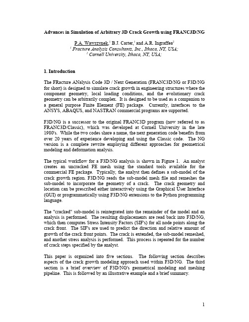
Advances in Simulation of Arbitrary 3D Crack Growth using FRANC3D/NG P.A. Wawrzynek,1 B.J. Carter,1 and A.R. Ingraffea21 Fracture Analysis Consultants, Inc., Ithaca, NY, USA;2 Cornell University, Ithaca, NY, USA;1. IntroductionThe FRacture ANalysis Code 3D / Next Generation (FRANC3D/NG or F3D/NG for short) is designed to simulate crack growth in engineering structures where the component geometry,local loading conditions,and the evolutionary crack geometry can be arbitrarily complex. It is designed to be used as a companion to a general purpose Finite Element(FE) package.Currently,interfaces to the ANSYS, ABAQUS, and NASTRAN commercial programs are supported.F3D/NG is a successor to the original FRANC3D program (now referred to as FRANC3D/Classic),which was developed at Cornell University in the late 1980's. While the two codes share a name, the next generation code benefits from over 20 years of experience developing and using the Classic code. The NG version is a complete rewrite employing different approaches for geometrical modeling and deformation analysis.The typical workflow for a F3D/NG analysis is shown in Figure 1. An analyst creates an uncracked FE mesh using the standard tools available for the commercial FE package. Typically, the analyst then defines a sub-model of the crack growth region. F3D/NG reads the sub-model mesh file and remeshes the sub-model to incorporate the geometry of a crack. The crack geometry and location can be prescribed either interactively using the Graphical User Interface (GUI) or programmatically using F3D/NG extensions to the Python programming language.The "cracked" sub-model is reintegrated into the remainder of the model and an analysis is performed. The resulting displacements are read back into F3D/NG, which then computes Stress Intensity Factors (SIF's) for all node points along the crack front. The SIF's are used to predict the direction and relative amount of growth of the crack front points. The crack is extended, the sub-model remeshed, and another stress analysis is performed. This process is repeated for the number of crack steps specified by the analyst.This paper is organized into five sections.The following section describes aspects of the crack growth modeling approach used within F3D/NG. The third section is a brief overview of F3D/NG's geometrical modeling and meshing pipeline. This is followed by an illustrative example and a brief summary.Figure 1. Typical workflow for a F3D/NG crack growth analysis.2. Modeling ApproachIn this section, key aspects of how F3D/NG operates and interacts with other programs are described.2.1 Sub-modelsF3D/NG supports the notion of a sub-model;remeshing for crack growth is confined to this sub-model. The sub-model approach is illustrated in Figure 2. All the supported FE packages have tools to define a sub-model.In a "real world" analysis, the size of a crack is small relative to the size of the structure. Confining the remeshing for crack growth to the sub-model greatly reduces the amount of data that needs to be transferred to, and processed by, F3D/ NG, thus speeding the crack growth process. It also allows the analyst to leave intact portions of a model with different structural idealizations(e.g.shell elements), complex boundary conditions (e.g., contact), or are just naturally and easily meshed with brick elements(F3D/NG remeshes with predominantly tetrahedral elements, as described below).Sub-modeling is used for mesh modification only; it does not affect the analysis strategy. That is, the remeshed sub-model is "plugged" back into the global model and the stress and deformation analysis is performed for the full composite model.This approach is not a sub-structuring or local/global analysismethodology. The sub-model can be redefined at any step of a crack growthanalysis.FRANC3D/NGFE mesh compatibilitymaintainedFRANC3D/NGremeshes a“sub-model”“global”modelFigure 2. The sub-modeling approached used in F3D/NG.2.2 Mesh File InterfaceThe main form of communication between F3D/NG and FE programs is through ASCII mesh description files. These are human-readable files that define a mesh, node coordinates, materials, and boundary conditions. These files use proprietary formats defined by the FE package vendors (.cdb, .inp, and .bnf formats for ANSYS, ABAQUS, and NASTRAN, respectively). F3D/NG expects a mesh file as input that describes an uncracked model or sub-model. It may also request a file of nodal temperatures in the case of thermal/mechanical loading, and possibly a file of nodal stresses if initial or residual stress fields are to be considered The output from the program is a new file that describes a mesh for a model or sub-model containing a newly inserted or newly extended crack (and possibly a file of interpolated nodal temperatures).Transferring a mesh description of a component between F3D/NG and a FE program is sub-optimal because mesh descriptions encode geometrical information incompletely.For example,if a portion of the surface of a component is curved, then the mesh model will have replaced that surface with a collection of planar or polynomial patches. This means that F3D/NG must use heuristic algorithms to reconstruct a description of the local geometry from the mesh data(a procedure described below).In most cases,the reconstructed geometry will be approximate.In theory,a better approach would be for the FE package to send F3D/NG geometrical data with the mesh data. In practice, however, this would introduce unwanted complexities. The format of mesh files varies among venders, but the main information they contain (node coordinates and element descriptions) is essentially the same among popular FE packages, and they describe a relatively simple data model.True geometrical information, in general,is much more complex and can vary markedly among vendors. Frequently, an analyst tasked with performing a crack growth investigation does not have easy access to a solid model description of a component and can more easily work with a mesh model. On balance,even though exchanging FE data introduces geometrical approximations, doing so makes F3D/NG a more flexible and useful tool than if it were tied to the geometrical information demanded by a specific FE package.2.3 Initial Flaw GeometryF3D/NG can be used to insert both zero volume flaws (cracks) and finite volume flaws (voids) into a model. Both types of flaws are defined as a collection of triangular cubic Bézier spline patches. Using spline patches to describe flaws means that very complex, doubly curved crack surfaces can be modeled. In most cases, however, an analyst will start by inserting an initial flaw with a relatively simple geometry and have it grow into a more complex shape.F3D/NG provides a "wizard" to specify an initial flaw shape, orientation, and location. One first selects from a small library of parameterized flaw shapes (e.g. elliptical crack, part-through crack, center crack, ellipsoidal flaw). Then one specifies translations and rotations to position the flaw.. The wizard provides visual feedback so that one can confirm the flaw is in the proper location. An image crack insertion wizard is shown in Figure 3.Notice in figure 3 that the wizard allows the analyst to work with the full elliptical crack shape, even though only about half the ellipse will ultimately be inserted into the part. The program computes the intersection of the flaw with the (in this case, doubly curved) surface and trims the unused portion of the flaw.. This means the same parameterized elliptical crack model can be used to define a wide range of fully embedded, surface, or corner crack geometries.2.4 Crack Region MeshingA variety of element types is used within F3D/NG for meshing near cracks. As illustrated in figure 4, 15-nodes wedge elements are used adjacent to a crack front. By default, eight wedge elements are used circumferentially around the crack front and these elements have the appropriate side-nodes moved to the quarter points,which allows the element to reproduce the theoretical1/√r stress distribution.The crack-front elements are surrounded by "rings" of 20-noded brick elements (two rings by default). Together, the wedge and brick elements comprise what is referred to as the crack front "template". The template is extruded along the crack front a shown in figure 5. This regular pattern of elements in the template is exploited when computing conservative integrals (e.g., J-integral and M-integral).Figure 3. An image from the flaw insertion wizard showing an elliptically shapedcrack being positioned in a gear tooth.The bulk of the sub-model is meshed with 10-noded tetrahedral elements. The triangular faces of the tetrahedral elements are not compatible with the quadrilateral faces of the brick elements;13-noded pyramid elements are used to transition from the template to the tetrahedra. Not all finite element packages support pyramid elements, so as an option the pyramid elements can be divided into two tetrahedra with the "hanging" node constrained.2.4 Computing Crack-front ParametersF3D/NG computes stress intensity factors using either a displacement correlation approach or an M-integral. It can also compute elastic strain energy release rates by way of a J-integral.In the displacement correlation approach,the finite-element-computed displacements for nodes on the crack faces are substituted into the theoretical expressions for the crack-front displacements fields written as functions of the stress-intensity factors.For a linear-elastic analysis, the J-integral is equivalent the total strain energy release rate. F3D/NG uses an equivalent domain formulation of the J-integral where the conventional contour formulation is replaced with a volume integral, which can be evaluated more accurately in a finite element contextThe M-integral, sometimes called the interaction integral, computes the energy release rates segregated by modes so the modal SIF's (K I,K II, and K III) can be computed.F3D/NG has M-integral formulations for both isotropic andorthotropic materials where the material axes can be oriented arbitrarily relative tothe crack front [1].quarter-point singular wedgecrack-front elements two or more “rings”of brick elementspyramids enforce compatibilitybetween brick and tetrahedral elements tetrahedral elements are used for the bulk of the volume meshFigure 4. Element types used to mesh the crack-front region.crack-front templateFigure 5. A crack-front template2.5 Crack GrowthWithin F3D/NG, crack growth is a five-step process:1.SIF’s are computed for all node points along the crack front.2.At each such point the direction and extent of growth is determined.3. A space curve is fit through the new crack-front points and, for the case of a surface crack, extrapolated, if necessary, to extend outside of the body.4.New Bézier patches are added to the crack surfaces.5.The extended crack is inserted into an uncracked mesh.By default, the Maximum Tensile Stress (MTS) criterion is used to predict the local direction of crack growth. One can also select a transition to a Maximum Shear Stress (MSS) criterion when the ratio of Mode II to Mode I is above a defined threshold.The relative amount of crack growth for points along the front, by default, is a ratio of the corresponding SIF's raised to an analyst specified power. This is analogous to evaluating the Paris crack growth rate equation for two points where both points are subjected to the same number of load cycles. In addition to a Paris type model, the NASGRO or an analyst supplied (piecewise linear in log/log space) crack growth rate equation can be used to determine relative amounts of growth.3. The FRANC3D/NG Geometry/Meshing PipelineThe core of the F3D/NG program is the geometrical modeling and meshing pipeline that adapts a FE mesh to insert a crack. This is a four-step process: surface facets and edge detection,geometry reconstruction,intersection computations, and meshing. These steps are described briefly in the following sections.3.1 Surface Facets and Edge DetectionAs mentioned above, F3D/NG takes as input a mesh description of model. The first step in the pipeline is to determine the FE facets that either make up the outer boundary of the sub-model or fall on a bi-material interface. Depending on the solid element type, the surface facets will have either a triangular or quadrilateral shape. Only element corner nodes are considered Quadrilateral element facets are further divided into two triangular facets yielding a planar- faceted, approximate geometrical description of the sub-model external and bi-material interface surfaces.The next step is to determine collections of the surface facets that can be grouped to form planar or gently curving regions that can be logically seen as a single surface, figure 6. The logical surfaces are bounded by "hard" edges. These are patch boundaries that one would perceive as making up a portion of a "sharp" edge of the model.Hard edges andoriginal FEM mesh triangular facetslogical surfacesFigure 6. Preliminary surface and edge detection.The primary heuristic used to identify sharp edges is to examine the angle between two adjacent surface patches. If the angle is below a threshold, thecommon boundary segment is flagged as a hard edge. Once all edges have been identified, strings of adjacent edges are determined and grouped to form circuits that form boundaries of logical surfaces.Exceptions to the patch grouping procedure are surfaces that fall on the interface between the sub-model and global model. These surfaces are retained as distinct patches so that nodal compatibility can be maintained when the sub-model is reinserted into the global mesh.3.2 Geometry ReconstructionThe FE facets give an approximate description of the surface geometry of the sub-model. A more accurate, but still approximate, geometry description is obtained by replacing the planar triangular facets with triangular cubic Bézier patches, which can represent doubly curved surfaces.These patches have ten control points so ten conditions must be given to define the geometry. Three conditions are given by the coordinates of the corners of the patches. Three more conditions are given by computing normals at all patch corners. Normals are computed as a weighted average of the planar facet normals for facets sharing the corner. The weights are given by the included patch angle at the corner point. If the corner falls on a hard edge, care is taken so that normals are not averaged across the edge. The final control point is selected to maintain quadratic precision of the surface interpolation [2].3.3 Intersection ComputationsAt this stage of the pipeline, both the component and the crack are represented as collections of triangular cubic Bézier patches.To"insert"the crack into a component,a search is made to find all intersections between crack and component patches [3,4]. For intersected crack patches, those parts of the patch inside the component and those outside are determined. The external parts are "trimmed", and the internal parts are added to the component model to form a composite crack/component model. The intersection curves, which are the crack mouth, become additional hard edges in the model.3.3 MeshingThe final stage in the pipeline is generating a FE mesh. Meshing is performed in four steps. First, FE nodes are generated along all hard edges. Second, triangular surface meshes are generated for all logical surfaces. Third, pyramid elements are generated adjacent to all quadrilateral boundary facets.Finally,a tetrahedral volume mesh is generated for the full sub-model.Generating nodes along the hard edges is an iterative process.First, a characteristic element size is determined for the ends of all hard edges. Thecharacteristic size will be the smaller of the shortest of all the adjacent hard edge lengths and the size of the finite element that was at this location before crack insertion. Node distributions along the edges are then determined such that there will be a linear variation in element sizes from one end of the edge to the other. If the rate of change of nodal spacing along any edge is greater than a threshold, then the longer of characteristic lengths at this edge's endpoints is reduced until the spacing is within tolerance. As the edge endpoint will also be an endpoint for other hard edges, the size reduction will require a regeneration of nodes for these edges. This might possibly cause these edges to violate the spacing transition tolerance, and the process is repeated iteratively until the node distributions along all edges fall within the tolerance.An advancing front meshing algorithm is used to generate surfaces meshes. One of two forms of this algorithm is used, depending on the geometry of the surface. If the surface is planar or nearly so, the surface boundary is mapped to a least squares fit plane,a2-D mesh is generated in this plane,and the internally generated node points are mapped back so that they fall on the appropriate Bézier patches. If the surface has significant curvature, then a computationally more expensive advancing front procedure is used where all the computations and intersection checks are performed using the3-D surface geometry[5].An advancing front meshing algorithm is used for volume meshing also. In this case tetrahedral elements are generated [6].4. ExampleFor a simple demonstration analysis,a"half-penny"surface crack has been inserted into a thick-walled cylinder subjected to combined tension and torsion loading. The left image of figure 7 shows the FE mesh with a high concentration of elements near the crack mouth. The center image shows a detail of the mesh on the surface of the crack. The right image shows the crack surface after one step of crack growth. The crack extension is non-planar due to the mixed-mode loading.Figure 7. Crack growth in a thick-walled cylinder: initial mesh (left), initial crack surface mesh (middle), crack surface mesh after one step of growth (right). Figure 8 shows a sequence of "cut-away" images illustrating the evolving crack geometry. The penultimate image shows that the crack front is automatically splitinto two fronts as the crack grows to the inner bore. The final image shows the final trace of the crack mouth on the surface of the cylinder.Figure 8. The geometry of the evolving non-planar crack geometry.5. SummaryF3D/NG is a program designed to simulate crack growth in engineering structures were the component geometry, local loading conditions, and the evolutionary crack geometry can be arbitrarily complex.It is designed to be used as a companion program to a general purpose FE package. Because stress analysis is performed by capable commercial packages, complex mechanics, such as contact and advanced material models, can be included in crack growth analyses.This paper has provided a brief overview of F3D/NG.Because of length restrictions many aspects of the program have been treated very superficially. Little mention has been made of the graphical user interface, which allows an analyst to be productive with a shallow learning curve. The paper does show, however,how geometrical modeling,computational fracture mechanics,and meshing capabilities have been combined to create a tool that provides an analyst with the capability to model realistically shaped cracks in real engineering structures subjected to realistic loads.AcknowledgementsWe gratefully acknowledge that the development of FRANC3D/NG was partially supported byAFRL/RXLMN, contract numbers FA6650-04-C-5212 and FA8650-07-C-5216, Drs. Pat Golden and Reji John technical monitors, and byNAVAIR,contract number N68335-08-C-0011,Mr.Ken Barlow technical monitor.References[1] L. Banks-Sills,P. Wawrzynek, B. Carter, A.Ingraffea, I. Hershkovitz, Methods for computing stress intensity factors in anisotropic geometries: Part II – arbitrary geometry, Eng Fracture Mech74 (8)(2007) 1293-1307[2] G. Farin, Curves and Surfaces for CAGD, Morgan Kaufmann Publishers, San Francisco, 2002[3] G. Müllenheim, On determining start points for a surface/surface intersection algorithm, Comp Aided Geometric Design 8 (1991) 401-408[4] C. Bajaj, C. Hoffmann, R. Lynch, J. Hopcroft, Tracing surface intersections, Comp Aided Geometric Design 5 (1988) 285-307[5] A. Miranda, L. Martha, P. Wawrzynek, A. Ingraffea, Surface mesh regeneration considering curvatures, Eng with Comp, Submitted December, 2007 [6] J. Cavalcante Neto, P. Wawrzynek, M. Carvalho, L. Martha, and A. Ingraffea, An algorithm for three-dimensional mesh generation for arbitrary regions with cracks, Eng with Comp 17 (2001) 75-9111。
SYSTEM AND METHOD FOR OPERATING IN VIRTUAL 3D SPAC

3DMAX自由立体显示功能的实现
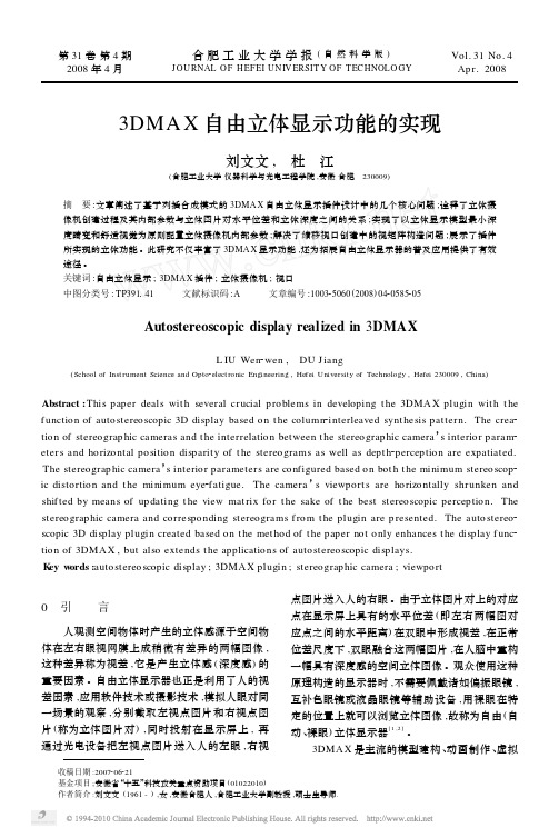
图1 位差与深度
片上的对应点在显示屏上所形成的理想位差尺度 s 应该在 ( - l/ 95 ~ l/ 105 ) 之内 , 此时 , 视者可以舒 适地将立体图片对融合成为一幅具有深度感的立 体图像 。
1 双眼能够融合的位差尺度及其深度感
第4期
刘文文 ,等 :3DMA X 自由立体显示功能的实现
587
主要显示对象包容球 ( 见图 2 上方的 3D 模型) 的 尺度 ,将显示模型从世界坐标系分别转换到左右 摄像机坐标系后进行相应的投射变换 , 再分别计 算显示对象上离左右摄像机最近点和最远点所构 成的最大正负位差值 ,根据 ( 1 ) 式计算出总立体 深度 ,其尺度应该与显示对象在显示表面上的尺 度相匹配 , 同时检验最大正负位差在 ( - l/ 95 ~ l/ 105 ) 之间 。 据此 ,针对透视投射 ,立体摄像机内部参数设 置为
点图片送入人的右眼 。由于立体图片对上的对应 点在显示屏上具有的水平位差 ( 即左右两幅图对 应点之间的水平距离) 在双眼中形成视差 ,在正常 位差尺度下 ,双眼融合这两幅图片 ,在人脑中重构 一幅具有深度感的空间立体图像 。观众使用这种 原理构造的显示器时 ,不需要佩戴诸如偏振眼镜 , 互补色眼镜或液晶眼镜等辅助设备 , 用裸眼在特 定的位置上就可以浏览立体图像 ,故称为自由 ( 自 动、 裸眼) 立体显示器[ 1 ,2 ] 。
2 立体摄像机创建以及内部参数设置
在 3DMA X 中 , 通过摄像机实现对空间的取 景 , 所谓立体摄像机就是由 2 台内部参数完全相 同摄像机的组合 。由于基于列插合成模式的自由 立体显示要求两摄像机截取的立体图片对没有垂 直位差 , 所以针对透视投射 ( Per spective ) 型摄像 机 , 应以两摄像机拍摄方向平行 、 摄像机 x 轴在 [4 , 5 ] 同一平面的方式构建立体摄像机 , 如图 2a 所 示 ,立体摄像机的内部参数为两摄像机之间的距 离 t ; 针对正交投射 ( Ort hograp hic ) 型摄像机 , 可 以两摄像机指向同一目标 、 摄像机 x 轴在同一平 面的方式构建立体摄像机 , 如图 2b 所示 , 立体摄 像机的内部参数为两摄像机的夹角 β 。再者 , 立 体显示内容在深度上应有最小的畸变 , 即整体深 度应该与显示表面上模型的尺度相匹配 。
湖南省长沙市平高教育集团2024-2025学年高三上学期八月联合考试英语试题(无答案)
2024年平高教育集团八月联合考试高三英语第一部分听力(共两节,满分30分)第一节(共5小题;每小题1.5分,满分7.5分)听下面5段对话。
每段对话后有一个小题,从题中所给的A、B、C三个选项中选出最佳选项。
听完每段对话后,你都有10秒钟的时间来回答有关小题和阅读下一小题。
每段对话仅读一遍。
1. What color is the dress the woman is trying on?A. Yellow.B. Orange.C. Blue.2. What is the man’s job probably?A. A novelist.B. A cartoonist.C. A reporter.3. What kind of occasion are the speakers probably celebrating?A. A wedding.B. A holiday.C. A birthday.4. How does the woman prefer to learn?A. By reading books.B. By watching videos.C. By using the Internet.5. Who was the man angry with?A. The cinema staff.B. The woman.C. Some other audiences.第二节(共15小题;每小题1.5分,满分22.5分)听下面5段对话或独白。
每段对话或独白后有几个小题,从题中所给的A、B、C三个选项中选出最佳选项。
听每段对话或独白前,你将有时间阅读各个小题,每小题5秒钟,听完后,各小题将给出5秒钟的作答时间。
每段对话或独白读两遍。
听第6段材料,回答第6、7题。
6. What are the speakers doing?A. Having a picnic.B. Preparing a meal.C. Shopping in a supermarket.7. What did the man want to eat at first?A. A salad.B. A sandwich.C. Noodles.听第7段材料,回答第8至10题。
FRANC3D_用户文献
学术论文
学术论文
• A 2d Multiscale Procedure For Fatigue Crack Nucleation(127页)
– 利用 FRANC3D 对微观模型进行任意形状三位裂 纹扩展模拟,并获得三种断裂模式的应力强度因 子。他的导师为康奈尔大学断裂力学组最权威的 教授——Anthony R. Ingraffea。
• Effects of Combined Loads on the Nonlinear Response and Residual Strength of Damaged Stiffened Shells(183-196页)
– NASA Langley Research Center – Lockheed Palo Alto Research Laboratory – 会 议 名 称 : FAA-NASA Symposium on the Continued Airworthiness of Aircraft Structures
• Determination Of Mixed-mode Stress Intensity Factors, Fracture Toughness, And Crack Turning Angle For Anisotropic Foam Mater ( 4936/4939/4941/4943/4950 页)
• Sub-modeling of Thermal Mechanical Fatigue Crack Propagation (55-85页)
– 使用 FRANC3D 对发动机涡轮叶片结构壁上贯穿 裂纹的损伤容限进行评估,使用了 FRANC3D 的 子模型技术,并考虑了温度的影响。
发动机应用案例
Visual Computer manuscript No. (will be inserted by the editor) Convex Contouring of Volume
Visual Computer manuscript No.(will be inserted by the editor)Convex Contouring of Volumetric Data Tao Ju1,Scott Schaefer1,Joe Warren1Department of Computer Science,Rice UniversityThe date of receipt and acceptance will be inserted by the editorAbstract In this paper we present a fast,table-driven isosurface extraction technique on volumetric data.Un-like Marching Cubes or other cell-based algorithms,the proposed polygonization generates convex negative space inside individual cells,enabling fast collision detection on the triangulated isosurface.In our implementation, we are able to perform over2million point classifica-tions per second.The algorithm is driven by an auto-matically constructed look-up table that stores compact decision trees by sign configurations.The decision trees determine triangulations dynamically by values at cell ing the same technique,we can perform fast, crack-free multi-resolution contouring on nested grids of volumetric data.The method can also be extended to ex-tract isosurfaces on arbitrary convex,space-filling poly-hedra.Keyword:contour,polygonization,implicit modeling 1IntroductionRecent advances in hardware technology of3D scanning and sensoring has brought about the generation of large-scale volumetric data such as MRI scans,CT scans and geological images.A common approach to visualize these volume datasets is to represent the data as implicit func-tions and construct polygonal approximations of isosur-faces,i.e.locus of points with some given function value. This process is often referred to as contouring.The con-toured surface partitions the whole volume into negative space(locus of points with lower function values)and positive space(locus of points with higher function val-ues).In many interactive applications,such as computer gaming and real-world simulations,navigation is con-fined to the negative space,therefore fast operations for checking the side of the main subject(e.g.the navigator) with respect to the contoured surface becomes critical.These operations are often referred to as collision detec-tions.Traditionally,contouring algorithms consider the data volume in uniform cubical cells and polygonize isosur-faces in each non-empty cell,i.e.,cells that are inter-sected by the isosurface.By doing so,the entire nega-tive space is decomposed into sub-spaces within individ-ual cells.Assuming that the negative space models free space,checking whether a point lies inside the free space can be greatly accelerated if the negative sub-space is convex within the enclosing cell.Note that this point-classification is the fundamental operation for computing collision detection with other convex objects.For exam-ple,an edge lies in the free space if for each cell it passes through,both endpoints of the line segment within that cell lie in the cell’s negative space(figure1left).This observation is not true if the negative space within the cell is non-convex(figure1right).Fig.1Edge classification in a signed square with two dif-ferent contours.The dashed lines indicate the contours,the gray areas represent negative space,and the dark gray lineis the edge to be checked.The most widely used cell-based algorithm is the March-ing Cubes(MC)algorithm introduced by Lorensen and Cline[7].MC generates triangles on isosurfaces within each cell based on a pre-computed table of positive/negative patterns(referred to as sign configurations hereafter)2Tao Ju etal.Fig.2Triangulations from theof cell corners.MC became popular for its fast polygo-nization and easy implementation due to its table-drivenmechanism.However,for some sign configurations,MCdoes not produce polygonizations that are consistentin topology with neighboring cells,and thus result insurface discontinuities[4].This drawback has sparkledextensive research on dis-ambiguation solutions[1],[4],[5],[10]and strategies to generate topologically correctpolygonizations[9].Although these solutions generatetopologically consistent isosurfaces,the resulting nega-tive space inside each cell is sometimes disconnected,andthus not convex.In this paper,we propose a fast table-driven cell-basedcontouring method that generate topologically consis-tent contours,while preserving convexity of the nega-tive space within each cell.The algorithm depends on acomposite look-up table that associates each sign con-figuration with a compact decision tree for dynamic tri-angulation of isosurface patches.The reason for the useof a decision tree is that the actual triangulation de-pends not only on the signs,but also on the magnitudeof corner values.The decision trees are pre-computed toensure a minimal number of tests in determining eachtriangulation.This technique can be extended without difficulty tomulti-resolution contouring.In most multi-resolutionapproaches,direct application of the cell-based contour-ing algorithm to a grid of non-uniform cells can resultin surface cracks,i.e.discontinuity between iso-surfacesgenerated from neighboring cells at different resolutions.Various multi-resolution frameworks have been proposedfor contouring on non-uniform grids[3],[8],[11],[12],[14],yet they involve special crack-patching strategies.Bloomenthal[2]proposes an adaptive contouring methodwhich requires run-time face tracing to maintain con-sistent contours for neighboring cells.We show that byconstructing look-up tables for transition cells using theabove algorithms,the same table-driven contouring methodcan be applied to non-uniform data to generate crack-free isosurfaces.The remainder of this paper is organized as follows.Afterreviewing the table-driven Marching Cubes algrorithm,we present the convex contouring algorithm on uniformgrids.Then we explain the automatic construction oflook-up tables in more detail.Next we extend the pro-posed technique to non-uniform grids to produce crack-free contour surfaces.We conclude by discussing otherpossible extensions and applications.2Marching Cubes and Look-up TablesMarching Cubes is a popular algorithm for extractinga polygonal contour from volumetric data sampled ona uniform3D grid.For each cell on the grid,the edgesintersected with the iso-surface are detected from signsat cell corners.The algorithm then forms triangles byconnecting intersections on those edges(referred to asedge intersections hereafter).To speed up the process,ituses a look-up table that establishes triangulations foreach sign configuration.Since there are8corners in acell,the look-up table contains256entries,four of whichare shown infigure2.Using the look-up table,the Marching Cubes algorithmcontours a cell in two steps:1.Look up the triangulation in the table by the signconfiguration,2.For each triangle,compute the exact location of eachvertex(edge intersection)from values at the cell cor-ners by linear interpolation.The Marching Cubes algorithm is fast because it uses ta-ble look-up to build polygonal contours.Unfortunately,the contoured surface generated by the original look-uptable in[7]may contain holes,since the triangular con-tour within each cell is not always consistent with thatof the neighboring cells(figure3).Although this problem wasfixed in later work,it re-veals another drawback of manually created tables.Theentries in the Marching Cubes’look-up table are con-structed by identifying15topologically distinct sign con-figurations and triangulating each case by hand.The lackof automation makes it susceptible to errors and diffi-cult to adapt to other polyhedrons.As we shall see,thelook-up tables used in convex contouring are constructedalgorithmically based on the topology and geometry ofgiven polyhedrons,and therefore minimizes possible er-rors.Convex3Fig.3Two the Marching Cubes topology.3Convex Contouring Using Look-up Tables The goal of convex contouring is to extract polygonal contours that enclose convex negative spaces within each cell.In this section,we will introduce the concept of con-vex contours and describe the proposed polygonization technique based on a pre-computed look-up table.Ex-amples of convex contouring will be presented together with performance comparison with the Marching Cubes algorithm.3.1Convex contourAssuming that the underlying implicit function is trilin-ear inside each cell,the convex hull of the negative space in a cell is the convex hull of all negative cell corners and edge intersections.The convex contour is the part of this convex hull that lies interior to the cell.In 2D,for exam-ple,the convex contour consists of interior line segments connecting edge intersections (i.e.,dashed lines in fig-ure 1left).In 3D,the convex contour consists of interior triangles whose vertices are edge intersections (figure 4left).Together with the triangles that fill the negative regions on cell faces (figure 4right),they constitute the convex hull of the negative space inside thecell.Fig.4Convex contour on the convex hull of the negative space.Note that the convex contour in a cell is outlined by linear convex contours on the faces of the cell (high-lighted in figure 4).Since the linear convex contour in a2D square is uniquely determined given the signs at the 4corners (allowing movement of the edge intersections along the edges),the polygonal convex contours from neighboring 3D cells always share the same linear con-tour on the common face.Hence convex contours always form topologically consistent isosurfaces.In figure 5,we show the convex contours for the same cells from figure 2.In comparison,we observe that the convex contour always encloses a connected,convex neg-ative space within the cell,whereas the contour from the Marching Cubes algorithm does not.Note that a convex contour is sometimes composed of multiple connected components,as shown in the rightmost cell of figure 5.Each of these connected piece of the contour is called a patch ,which may contain multiple holes (such as the center left cell in figure 5).Each hole on the patch is surrounded by a ring of linear convex contours that can be detected by the signs at the corners.Hence a look-up table for patch boundaries can be constructed automat-ically for each sign configuration.3.2Triangulation and Decision treesUnfortunately,although the boundary of the patches on the convex contour is unique for each sign configuration,the actual polygonization is not.In fact,different scalar values at cell corners,which determine the location of edge intersections,may modify the shape of the convex hull and result in different triangulation of the convex contour.As illustrated in figure 6,two cells that share the same sign configuration,but with different scalars at cell corners,result in different triangulated convexcontours.Fig.6Triangulation in cells with different scalar values at corners.Edge intersections are indicted by gray dots.To determine the correct triangulation based on the lo-cation of edge intersections,one could apply a full-scale convex-hull algorithm to compute the convex hull of the negative space.However,such algorithms are too gen-eral for our purposes,since we want only the part of this convex hull that lies interior to the cell.Instead,we can take advantage of the fact that the topology of the boundary is known for each patch on the convex contour.In fact,we can construct a set S of all possible triangu-lations for each patch.For example,figure 6shows the4Tao Ju etal.Fig.5Convex contours in cells withonly two possible triangulations for the convex contour ofthat sign configuration,since the contour contains a sin-gle4-sided patch.According to Euler’s polygon divisionproblem[6],there are(2n−4)!(n−1)!(n−2)!ways to triangulate an−sided patch into n−2triangles.In fact,this size ofS can be further reduced if we realize that the verticesof these triangles are restricted tofixed cell edges,hencesome triangulations will never appear on the convex hullof negative space.We will discuss this process in detailwhen we describe how the look-up table is constructed.Now we can think of the triangulation problem as thefollowing:given the exact locations of the edge inter-sections,choose an appropriate triangulation from S sothat the triangles satisfy the convex hull property(i.e.,all edge intersections and negative corners lie on one sideof the triangle).Hence we need a fast method to differ-entiate the correct triangulation from others by lookingat the edge intersections.Assuming that triangles on theconvex contour face inside the convex hull of the nega-tive space,we can do this by the following4-point test:given four distinct edge intersections V1,V2,V3,V4,if V4lies on the front-facing side of the triangle(V1,V2,V3),then the inverted triangle(V1,V3,V2)does not belongto the convex contour(figure7left).Similarly,triangles(V1,V2,V4),(V2,V3,V4)and(V3,V1,V4)do not satisfythe convex hull property.Otherwise,by symmetry,weclaim that triangles(V1,V2,V3),(V1,V4,V2),(V2,V4,V3)and(V1,V3,V4)do not lie on the convex contour(figure7right).Note that if all vertices lie on the same plane,either choice can be made.V1V2V3V4V1V2V3V4Fig.7Four-point test with vertices V1,V2,V3,V4.Each4-point test on the edge intersections rules outthose from the set S of all possible triangulations thatcontain any of the four back-facing triangles.Since anytwo triangulations differ at least in the triangles sharedby one of the boundary edge,the correct triangulationcan be distinguished from every other triangulation in Sthrough appropriate4-point tests.For best performance,a decision tree can be built to distinguish each triangula-tion through a minimal set of tests.An example of sucha decision tree is shown infigure8for a5-sided patch.At each node,the remaining triangulations are shownand the4-point test is represented by indices of the fourvertices(the order is shown at the top left corner).If thefourth vertex lies on the front-facing side of the triangleformed by thefirst three vertices(in order),we take theleft branch.Otherwise,we follow the right branch.Theprocess stops at a leaf node,where a single triangulationisleft.2,4,5,13,4,5,12,3,4,52,3,5,11,2,3,412345Fig.8A decision tree using4-point test for5-sided patches.Since the construction of decision trees is based on theoriginal set S,they can be pre-computed and optimizedfor every patch in each sign configuration.As we shallsee,the maximum depth of all these decision trees is5and the average tree depth is1.88.In other words,thecorrect triangulation of the convex contour in a cubic cellcan be determined by performing a maximum of5point-face trials on the edge intersections,and on average nomore than2trials.3.3The look-up tableThe look-up table contains256entries,one for each signconfiguration of a cubic cell.In each entry,the look-uptable stores the decision trees computed for each patchConvex Contouring of Volumetric Data5 Fig.9Two screen shots of a real-time navigation application using a convexly contoured terrain.by traversing the nodes in the decision trees in pre-order. Each non-leaf node contains a4-point test,and each leaf node stores a triangulation.The edge intersections in4-point tests and triangulations are represented by indices of the edges on which they lie.Two example entries in this table are shown in table1,with their correspond-ing sign configurations and edge indexing drawn on the right.3.4Contouring by table look-upsIn comparison with the Marching Cubes algorithm,con-vex contouring extracts the polygonal contour in a cell in two steps:1.Look up the decision trees(one for each patch)in thetable by the signs at the cell corners,2.For each decision tree,perform4-point tests on spec-ified edge intersections until arriving at a single tri-angulation.Fig.10Convex contouring on volumetric data.Infigure10,two sets of volumetric data generated by scan-conversion of polygonal models are contoured us-ing the new method.Observe that the edges on the sur-face are manifold and the contour is crack-less.Since the negative space inside each non-empty cell is convex, collision detection can be localized into cells and there-fore become independent of the grid size.Figure9shows two screen shots of a real-time navigation program in which the movement of the viewer is confined within the negative space.The terrain is an iso-surface constructed using convex contouring on a256cubic grid.On a con-sumer level PC machine(dual1.5GHz processors with 2.5G memory),we achieved over2million point classifi-cations per second.As we mentioned before,the average number of tests used to determine triangulation for each patch is less than2.Hence we can perform convex contouring on vol-umetric data with speed comparable to the Marching Cubes algorithm.In table2,the performance of con-vex contouring is compared with that of the Marching Cubes for contouring the terrain infigure9on differ-ent grid sizes.We also compared the average number of triangles generated in each cell in both methods.Notice that convex contouring generates on average only about 2%more triangles than the Marching Cubes algorithm. These extra triangles are needed to preserve the convex-ity of the negative space.Grid Size Marching Cubes Convex Contouring 1283125ms141ms2563781ms907ms51232109ms2437msAvg.Triangles 3.181 3.257Table2Comparison of total contouring time and average number of triangles per cell in convex contouring and the Marching Cubes.6Tao Ju et al.Index Table Entry Cell Configuration171{1,9,12,7}→4-point test{{1,9,7},{9,12,7}}→Triangulation{{1,9,12},{1,12,7}}123456789101112125{1,3,6,12}→4-point test in parent node{1,12,10,2}→4-point test in left child{{1,3,12},{1,12,2},{3,6,12},{12,10,2}}{{1,3,12},{1,12,10},{1,10,2},{3,6,12}}{1,12,10,2}→4-point test in right child{{1,3,6},{1,6,12},{1,12,2},{12,10,2}}{{1,3,6},{1,6,12},{1,12,10},{1,10,2}}123456789101112Table1Two example entries in the look-up table.Each entry is a list of triangulations(each stored as a list of triangles) and4-point tests(each stored by the indices of the vertices)traversed from the decision tree in pre-roder.4Automatic Construction of Look-up TablesIn this section,we will review the table construction pro-cess in more detail.For a given sign configuration,we first detect the patch boundaries as a group of rings of linear contours.Then,for each patch,we construct the set of all possible triangulations that could take place on the convex hull of the negative space.Finally,an opti-mal decision tree is built for every patch detected on the contour.The look-up table can be found on the web at /jutao/research/contour tables/.4.1Detection of patch boundariesA patch on the convex contour in a cubic cell is bounded by linear convex contours on cell faces.These linear con-tours form single or multiple rings that surround the ”holes”of the patch.Since the linear convex contours are unique on each cell face for a given sign configura-tion,a single ring can be constructed using the following tracing strategy:starting from a cell edge that exhibits a sign change(where an edge intersection is expected) and facing the positive end,look for the next edge with a sign change by turning counter-clockwise on the face boundary.Repeat the search process until it returns to the starting edge,when a closed ring is formed(seefigure 11).Notice that face-tracing produces oriented linear convex contours on each cell face.Each linear contour on the cell face is directed so that the negative region on that face lies to its left when looking from outside.There-fore the triangles on the convex contour of the cell that share these linear contours will face towards the nega-tive space.The orientation of the rings are importantfor linear contours already built,and dashed arrows indicate the tracing route.determining the set of possible triangulations that share the same patch boundary.Similar tracing techniques have been described by nu-merous authors in[2],[9],[13],in which convexity of the negative region on each cell face is preserved.These algo-rithms construct a single ring for each patch boundary. However,the problem remains on how to group multiple rings to form the boundary of a multiple-genus patch (such as the center left cell infigure5).Although such patches arise in only4cases among256sign configura-tions,they may appear much more often in other non-cubic cells(such as transition cells in multi-resolution grids,see Section6).We need to be able to identify these cases automatically from the sign configuration and group the rings appropriately.By definition,a patch is a continuous piece on the con-vex hull of negative space.Hence it also projects onto a continuous piece of regions on the cell faces.These regions are positive areas that surround positive cor-Convex Contouring of Volumetric Data7ners connected by cell edges.Therefore the boundary of each patch on the convex contour isolates a group of positive corners that are inter-connected by cell edges. The previous face-tracing algorithm could be modified so that rings constructed around a same edge-connected component of positive corners are grouped to form the boundary of a single patch.This rule is demonstrated in figure12.In the top left cell,two rings of linear contours form the boundary of two patches,due to the presence of two isolated positive corners.In the top right cell,where there is only one edge-connected component of positive corners,the two rings are grouped to form the bound-ary of a single cylinder-like patch.The connectivity of the positive corners in these two cells are illustrated at the bottom offigure12.In contrast,face-tracing without ring-grouping would give the same result in both cells, thus violating the convex hull property in the secondcell.Fig.lighted)to form boundaries of patches.Positive corners are colored gray.Bottom:Connectivity graph of positive corners 4.2Pre-triangulation of Convex ContourThe set of possible triangulations for a patch with an oriented boundary topology can be enumerated by re-cursive algorithms.However,this often results in redun-dant triangulations that never appear on the convex con-tour.For example,the genus-2patch in the center left cell infigure5can be triangulated in only one way on the convex hull of the negative space,regardless of the magnitudes of scalar values at the corners.In contrast, brute-force enumeration would return21possible trian-gulations for an arbitrary genus-2patch with two trian-gular holes.The key observation is that,the patches on the convex contour are not arbitrary patches,their ver-tices(edge intersections)are restricted tofixed edges on the cell.These spacial restrictions limit the number of possible triangulations that could occur on the convex contour.For fast polygonization at run-time,we hope to pre-triangulate each patch as much as possible during table construction,based only on the sign configuration. By the convex hull property,the half-space on the front-facing side of a triangle on the convex contour must con-tain(or partially contain)every other cell edge that ex-hibits a sign change.Note that the three vertices of the triangle can move only along threefixed cell edges,this half-space is always contained in the union of the half-spaces formed when the three vertices are at the ends of their cell edges.Hence we have a way to identify triangles that will not appear on the convex contour:given three cell edges(C1,C2),(C3,C4)and(C5,C6)(C i are cell cor-ners),construct border triangles,i.e.,triangles formed by one end of each edge in order(such as(C1,C3,C5)).If there is an edge on the cell exhibiting a sign change that lies completely to the back of all non-degenerate border triangles,any triangle whose vertices belong to these three edges(in order)will not lie on the convex con-tour.This idea is illustrated infigure13.The highlighted cell edge on the left exhibits a sign change,and lies to the back of all the border triangles constructed from the three dashed edges(E1,E2,E3).Hence the dashed trian-gle formed by intersections on those edges never appears on the convex contour.In contrast,the highlighted cell edge on the right lies partially to the front of at least one of the border triangles formed by the edges(E1,E2,E3), hence the dashed triangle may exist in the triangulation of the convex contour.E1E2E3E1E2E3Fig.13Identifying triangles that do not lie on the convex contour.By eliminating triangulations that contain these ineli-gible triangles,we can trim down the space of possible triangulations.For example,the number of remaining triangulations for thefirst three cells infigure5are re-spectively4,1and4.4.3Construction of decision treesEven after pre-triangulation,some patches still have many potential triangulations on the convex hull of the nega-tive space.To speed up the polygonization at run-time,8Tao Ju et al.we can pre-compute a set of4-point tests on the vertices of the patch(edge intersections)to distinguish between the remaining triangulations.These tests can be orga-nized in a decision tree structure,introduced in the last section.Different sets of tests result in differently shaped decision trees.To obtain optimal performance,we imple-ment a search algorithm that looks for the optimal set of tests that produces a decision tree with the small-est depth.Since each of the two outcomes of a single test eliminates a non-intersecting subset of the remain-ing triangulations,the minimal depth of the correspond-ing decision tree is lower bounded by log2N,where N is the total number of triangulations.For example,the depth of an optimized decision tree for a patch of length 4,5and6are1,3and5respectively.Further computa-tion reveals that the maximum length of a patch(which can not be pre-triangulated)in a cubic cell is6;hence any patch can be triangulated within5point-face trials on thefly by walking down the pre-computed decision tree.On average,however,it only takes1.88tests to de-termine the triangulation of a patch,due to infrequent occurrence of large patches and the reduced triangula-tion space as a result of pre-triangulation.5Multi-resolution Convex ContouringIn volume visualization,the number of polygons gener-ated by uniform contouring easily exceeds the capacity of modern hardware.For real-time applications,it is often advantageous to display the geometry at different lev-els of detail depending on the distance from the viewer. This technique has the advantage that it speeds up the rendering process without sacrificing much visual accu-racy.By using a view-dependent approach,the grid is contoured at different resolutions depending on the dis-tance from the navigator.In particular,we can create a series of nested bounding boxes centered at the viewer, with the grid resolution decreasing by a factor of2.A2D example of this multi-resolution framework is shown infigure14left,in which a circle is contoured using cell grid at two different resolutions.When the coarse cells at the top meet thefine cells at the bottom,the con-tour in the coarse cells need to be consistent with the contour from the neighboringfine cells on the common edges.We call these coarse cells transition cells,which are adjacent to cells at afiner resolution.A2D transition cell thus hasfive corners andfive edges,as shown in the middle offigure14.By connecting edge intersections on each cell edge,the transition cells can be contoured in a way similar to a regular4-corner cell,yielding consistent contours with the adjacentfine cells.Some of the con-toured example are shown infigure14right.Notice that the convexity of the negative region is still preserved in each transition cell.In3D,a transition cell between two resolutions is either adjacent to twofine cells on an edge,or adjacent to four fine cells on a face(seefigure15left).These two types of cells can be regarded as convex polyhedrons with9 corners(figure15center)and13corners(figure15right) respectively.Since the previous discussion on regular cells applies to any convex polyhedron,we can also build look-up ta-bles and perform convex contouring on these transition cells.In this way,crack-free surfaces can be contoured on nested grids within the same framework as uniform contouring.5.1Convex contours in transition cellsAs in a regular cell,the convex contour inside a tran-sition cell is outlined by the linear contours on the cell faces.Since the linear convex contour is unique on each face for a given sign configuration,the boundary of patches on the convex contour can be pre-computed using the proposed face-tracing algorithm.At the top offigure16, the oriented boundaries of patches in different transition cells are detected and drawn as dashed arrows.Since con-vex contours from neighboring cells in a multi-resolution grid always share the same linear contour on the com-mon face as their boundaries,topological consistency is preserved everywhere on the contouredsurface.Fig.16Patch boundaries(top)and triangulation(bottom) in three transition cells.By pre-computing optimal decision trees for each patch, the triangulation can be determined by applying succes-sive4-point tests on the edge intersections.At the bot-tom offigure16,patches detected from the cells on the top are triangulated on the convex hull of the negative space.However,due to the presence of four co-planar faces on a13-corner cell,this convex hull could degener-ate onto a plane(figure17left).To determine the correct triangulation of the convex contour on the degenerate convex hull,we introduce an outward perturbation to。
hfss_full_book_V121_1.pdf
1-3
2. Microwave Examples
– Magic T
2-1
– Microwave Coax Bend
2-2
– 180 Ring Hybrid
2-3
– Coax Stub
2-4
– Microstrip Wave Ports
2-5
– Bandpass Filter
2-6
3. Signal Integrity
NOTE: You should make backup copies of all HFSS projects created with a previous version of the software before opening them in HFSS 12
ANSYS, Inc. Proprietary © 200190 ANSYS, Inc. All rights reserved.
– The name HFSS stands for High Frequency Structure Simulator. Ansoft pioneered the use of the Finite Element Method (FEM) for EM simulation by developing/implementing technologies such as tangential vector finite elements, adaptive meshing, and Adaptive Lanczos-Pade Sweep (ALPS). Today, HFSS continues to lead the industry with innovations such as Modes-to-Nodes and Full-Wave Spice™.
- 1、下载文档前请自行甄别文档内容的完整性,平台不提供额外的编辑、内容补充、找答案等附加服务。
- 2、"仅部分预览"的文档,不可在线预览部分如存在完整性等问题,可反馈申请退款(可完整预览的文档不适用该条件!)。
- 3、如文档侵犯您的权益,请联系客服反馈,我们会尽快为您处理(人工客服工作时间:9:00-18:30)。
position and orient crack crack-front template parameters
Surface Meshes after Crack Insertion
crack surface mesh as viewed from inside the model
11
Crack-Front Element Types
13
Embedded Penny Crack
1 0.8 0.6 0.4 % error 0.2 0 -0.2 -0.4 -0.6 -0.8 -1 normalized crack front le ngth 0 0.2 0.4 0.6 0.8 1 far-field traction values crack face pressure values
Fretting crack initiates at the edge of contact
24
* FEM model courtesy of NAVAIR
FRANC3D sub-model
open crack closed crack Deformed model plotted in ANSYS 23
Dovetail Attachment Crack
FRANC3D sub-model
Contact conditions Global FEM model* maintained during crack growth
crack size/shape parameters
position and orient crack crack-front template parameters
Crack Insertion Wizard (Middle-Crack Flaw)
crack size/shape parameters
after 21 steps of automatic crack growth
6
FRANC3D Typical Work Flow
ANSYS, ABAQUS, or NASTRAN interactive ANSYS, ABAQUS, or NASTRAN background
Build/analyze global model Define sub-model
12
Stress Intensity Factor Computations
SIF’s are computed with the M-integral (interaction integral) for isotropic and generally anisotropic materials.
16
A simple PyF3D Program
import PyF3D # file names for the models uncracked_fname = "minidisk_submodel.cdb“ fname_base = "minidisk_crack" # lists of crack size parameters a_sizes = [0.0160, 0.0320, 0.0480, 0.0640, 0.0787, 0.2362, 0.3937] b_sizes = [0.0160, 0.0787, 0.2362, 0.3937] app = PyF3D.F3DApp() # loop through the crack size matrix for a in a_sizes: for b in b_sizes: # skip cases with really #bad aspect ratios if b > 0.2 and a < 0.065: continue # create a flaw object flaw = PyF3D.Flaw("Ellipse",[a,b]) flaw.Translate([0.499,4.179,-.374]) flaw.Rotate(1,"Y",90.0) flaw.Rotate(2,"Z",-53.61) # open an uncrack model, insert the flaw app.OpenModel(uncracked_fname) app.InsertFlaw(flaw) # generate a new file name like: # minidisk_crack_160_320.fdb fname = "%s_%d_%d.fdb" % \ (fname_base,int(a*1000),int(b*1000)) # save the file app.SaveModel(fname)
2
Acknowledgements
Fracture Analysis Consultants gratefully acknowledges the following support for the development of FRANC3D/NG: AFRL/RXLMN, Contract #’s,FA6650-04-C5212 and FA8650-07-C-5216 Drs. Pat Golden and Reji John TPOC’s NAVAIR, Contract# N68335-08-C-0011 Mr. Ken Barlow TPOC
Advances in Simulation of Arbitrary 3D Crack Growth using FRANC3D/NG
Drs. Paul “Wash” Wawrzynek,1 Bruce Carter,1 and Anthony Ingraffea2
Analysis Consultants, Inc., Ithaca, NY 2 Cornell University, Ithaca, NY
± 1% error
14
Penny Surface Crack
1.4 1.35
2H
FRANC3D
1.3
KI MPa.sqrt(m)
Raju-Newman f3dng f3dng - refined mesh
2c
1.25 1.2 1.15 1.1 1.05 1 0 0.2 0.4 0.6 0.8 1
17
A Simple Crack Growth Analysis
tension/torsion cylinder with an initial surface flaw initial mesh
crack
crack surface mesh
cutaway view
non-planar automatic crack growth
quarter-point singular wedge crackfront elements tetrahedral elements are used for the bulk of the volume mesh
two or more “rings” of brick elements pyramids enforce compatibility between brick and tetrahedral elements
7
Wizards to Define Initial Cracks (elliptical flaw)
crack size/shape parameters
position and orient crack crack-front template parameters
Crack Insertion Wizard (Part-Through Flaw)
Stress Analysis
displacements
uncracked model
temperatures
model with initial crack model with extended crack
FRANC3D/NG Insert crack(s) (remesh)
Compute stress intensity factors Extend crack(s) (remesh)
Fracture Analysis Consultants, Inc.
1 Fracture
Outline • Introduction • Overview of FRANC3D/NG • Stress intensity factor examples • Crack growth examples • Summary
3
FRANC3D / Next Generation
• FRANC3D/NG is an all new version of the FRANC3D crack growth simulation program. • FRANC3D/NG adaptively remeshes a finite element model to simulate crack growth. • FRANC3D/NG is designed to work in conjunction with a commercial finite element program. Currently ANSYS, ABAQUS, and NASTRAN are supported.
4
Global and Sub-models
“global” model FRANC3D/NG remeshes a “sub-” model
FRANC3D/NG
FE mesh compatibility maintained
initial corner crack
5
Crack Growth
Stress Intensity Factors are computed and used to predict the direction and relative extent of crack growth