MATLAB-Simulink基础
matlab simulink设计与建模-概述说明以及解释

matlab simulink设计与建模-概述说明以及解释1.引言1.1 概述概述部分的内容可以描述该篇文章的主题和内容的重要性。
可以参考以下写法:引言部分首先概述了文章的主要内容和结构,主要涉及Matlab Simulink的设计与建模方法。
接下来,我们将详细介绍Matlab Simulink 的基本概念、功能和应用,并探讨其在系统设计和仿真建模中的重要性。
本文旨在向读者提供一种全面了解Matlab Simulink的方法,并帮助他们在实际工程项目中运用该工具进行系统设计和模拟。
通过本文的阅读,读者将能够深入了解Matlab Simulink的优势和特点,并学会如何使用其开发和设计各种复杂系统,从而提高工程的效率和准确性。
在接下来的章节中,我们将重点介绍Matlab Simulink的基本概念和设计方法,以及实际案例的应用。
最后,我们将通过总结现有的知识和对未来发展的展望,为读者提供一个全面的Matlab Simulink设计与建模的综合性指南。
1.2文章结构1.2 文章结构本文将以以下几个部分展开对MATLAB Simulink的设计与建模的讨论。
第一部分是引言部分,其中概述了本文的主要内容和目的,并介绍了文章的结构安排。
第二部分是正文部分,主要包括MATLAB Simulink的简介和设计与建模方法。
在MATLAB Simulink简介部分,将介绍该软件的基本概念和功能特点,以及其在系统设计和建模中的优势。
在设计与建模方法部分,将深入讨论MATLAB Simulink的具体应用技巧和方法,包括系统建模、模块化设计、信号流图、仿真等方面的内容。
第三部分是结论部分,主要总结了本文对MATLAB Simulink设计与建模的讨论和分析,并对其未来的发展方向进行了展望。
通过以上结构安排,本文将全面介绍MATLAB Simulink的设计与建模方法,以期为读者提供一个全面而系统的了解,并为相关领域的研究和应用提供一些借鉴和参考。
matlab simulink-实验1-simulink入门说明书
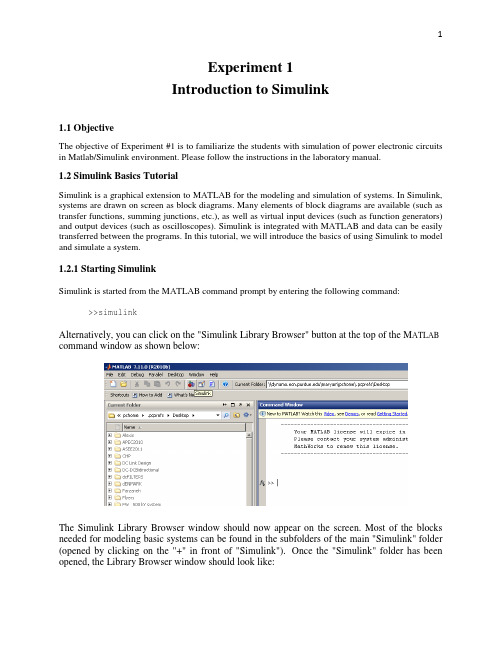
Experiment 1Introduction to Simulink1.1 ObjectiveThe objective of Experiment #1 is to familiarize the students with simulation of power electronic circuits in Matlab/Simulink environment. Please follow the instructions in the laboratory manual.1.2 Simulink Basics TutorialSimulink is a graphical extension to MATLAB for the modeling and simulation of systems. In Simulink, systems are drawn on screen as block diagrams. Many elements of block diagrams are available (such as transfer functions, summing junctions, etc.), as well as virtual input devices (such as function generators) and output devices (such as oscilloscopes). Simulink is integrated with MATLAB and data can be easily transferred between the programs. In this tutorial, we will introduce the basics of using Simulink to model and simulate a system.1.2.1 Starting SimulinkSimulink is started from the MATLAB command prompt by entering the following command: >>simulinkAlternatively, you can click on the "Simulink Library Browser" button at the top of the M ATLAB command window as shown below:The Simulink Library Browser window should now appear on the screen. Most of the blocks needed for modeling basic systems can be found in the subfolders of the main "Simulink" folder (opened by clicking on the "+" in front of "Simulink"). Once the "Simulink" folder has been opened, the Library Browser window should look like:1.2.2 Basic ElementsThere are two major classes of elements in Simulink: blocks and lines. Blocks are used to generate, modify, combine, output, and display signals. Lines are used to transfer signals from one block to another. BlocksThe subfolders underneath the "Simulink" folder indicate the general classes of blocks available for us to use:•Continuous: Linear, continuous-time system elements (integrators, transfer functions, state-space models, etc.)•Discrete: Linear, discrete-time system elements (integrators, transfer functions, state-space models, etc.)•Functions & Tables: User-defined functions and tables for interpolating function values•Math: Mathematical operators (sum, gain, dot product, etc.)•Nonlinear: Nonlinear operators (coulomb/viscous friction, switches, relays, etc.)•Signals & Systems: Blocks for controlling/monitoring signal(s) and for creating subsystems•Sinks: Used to output or display signals (displays, scopes, graphs, etc.)•Sources: Used to generate various signals (step, ramp, sinusoidal, etc.)Blocks have zero to several input terminals and zero to several output terminals. Unused input terminals are indicated by a small open triangle. Unused output terminals are indicated by a small triangular point. The block shown below has an unused input terminal on the left and an unused output terminal on the right.LinesLines transmit signals in the direction indicated by the arrow. Lines must always transmit signals from the output terminal of one block to the input terminal of another block. One exception to this is that a line can tap off of another line. This sends the original signal to each of two (or more) destination blocks, as shown below:Lines can never inject a signal into another line; lines must be combined through the use of a block such as a summing junction.A signal can be either a scalar signal or a vector signal. For Single-Input, Single-Output systems, scalar signals are generally used. For Multi-Input, Multi-Output systems, vector signals are often used, consisting of two or more scalar signals. The lines used to transmit scalar and vector signals are identical. The type of signal carried by a line is determined by the blocks on either end of the line.1.2.3 Building a SystemTo demonstrate how a system is represented using Simulink, we will build the block diagram for a simple model consisting of a sinusoidal input multiplied by a constant gain, which is shown below:This model will consist of three blocks: Sine Wave, Gain, and Scope. The Sine Wave is a Source Block from which a sinusoidal input signal originates. This signal is transferred through a line in the direction indicated by the arrow to the Gain Math Block. The Gain block modifies its input signal (multiplies it by a constant value) and outputs a new signal through a line to the Scope block. The Scope is a Sink Block used to display a signal (much like an oscilloscope).We begin building our system by bringing up a new model window in which to create the block diagram. This is done by clicking on the "New Model" button in the toolbar of the Simulink Library Browser (looks like a blank page).Building the system model is then accomplished through a series of steps:1.The necessary blocks are gathered from the Library Browser and placed in the model window.2.The parameters of the blocks are then modified to correspond with the system we are modeling.3.Finally, the blocks are connected with lines to complete the model.Each of these steps will be explained in detail using our example system. Once a system is built, simulations are run to analyze its behavior.Gathering BlocksEach of the blocks we will use in our example model will be taken from the Simulink Library Browser. To place the Sine Wave block into the model window, follow these steps:1.Click on the "+" in front of "Sources" (this is a subfolder beneath the "Simulink" folder) todisplay the various source blocks available for us to use.2.Scroll down until you see the "Sine Wave" block. Clicking on this will display a shortexplanation of what that block does in the space below the folder list:3. To insert a Sine Wave block into your model window, click on it in the Library Browser and drag the block into your workspace.The same method can be used to place the Gain and Scope blocks in the model window. The "Gain" block can be found in the "Math" subfolder and the "Scope" block is located in the "Sink" subfolder. Arrange the three blocks in the workspace (done by selecting and dragging an individual block to a new location) so that they look similar to the following:Modifying the BlocksSimulink allows us to modify the blocks in our model so that they accurately reflect the characteristics of the system we are analyzing. For example, we can modify the Sine Wave block by double-clicking on it. Doing so will cause the following window to appear:This window allows us to adjust the amplitude, frequency, and phase shift of the sinusoidal input. The "Sample time" value indicates the time interval between successive readings of the signal. Setting this value to 0 indicates the signal is sampled continuously.Let us assume that our system's sinusoidal input has:•Amplitude = 2•Frequency = pi•Phase = pi/2Enter these values into the appropriate fields (leave the "Sample time" set to 0) and click "OK" to accept them and exit the window. Note that the frequency and phase for our system contain 'pi' (3.1415...). These values can be entered into Simulink just as they have been shown.Next, we modify the Gain block by double-clicking on it in the model window. The following window will then appear:Note that Simulink gives a brief explanation of the block's function in the top portion of this window. In the case of the Gain block, the signal input to the block (u) is multiplied by a constant (k) to create the block's output signal (y). Changing the "Gain" parameter in this window changes the value of k.For our system, set k = 5. Enter this value in the "Gain" field, and click "OK" to close the window.The Scope block simply plots its input signal as a function of time, and thus there are no system parameters that we can change for it. We will look at the Scope block in more detail after we have run our simulation.Connecting the BlocksFor a block diagram to accurately reflect the system we are modeling, the Simulink blocks must be properly connected. In our example system, the signal output by the Sine Wave block is transmitted to the Gain block. The Gain block amplifies this signal and outputs its new value to the Scope block, which graphs the signal as a function of time. Thus, we need to draw lines from the output of the Sine Wave block to the input of the Gain block, and from the output of the Gain block to the input of the Scope block.Lines are drawn by dragging the mouse from where a signal starts (output terminal of a block) to where it ends (input terminal of another block). When drawing lines, it is important to make sure that the signal reaches each of its intended terminals. Simulink will turn the mouse pointer into a crosshair when it is close enough to an output terminal to begin drawing a line, and the pointer will change into a double crosshair when it is close enough to snap to an input terminal. A signal is properly connected if its arrowhead is filled in. If the arrowhead is open, it means the signal is not connected to both blocks. To fix an open signal, you can treat the open arrowhead as an output terminal and continue drawing the line to an input terminal in the same manner as explained before.Properly Connected SignalWhen drawing lines, you do not need to worry about the path you follow. The lines will route themselves automatically. Once blocks are connected, they can be repositioned for a neater appearance. This is done by clicking on and dragging each block to its desired location (signals will stay properly connected and will re-route themselves).After drawing in the lines and repositioning the blocks, the example system model should look like:In some models, it will be necessary to branch a signal so that it is transmitted to two or more different input terminals. This is done by first placing the mouse cursor at the location where the signal is to branch. Then, using either the CTRL key in conjunction with the left mouse button or just the right mouse button, drag the new line to its intended destination. This method was used to construct the branch in the Sine Wave output signal shown below:The routing of lines and the location of branches can be changed by dragging them to their desired new position. To delete an incorrectly drawn line, simply click on it to select it, and hit the DELETE key.1.2.4. Running SimulationsNow that our model has been constructed, we are ready to simulate the system. Before starting simulation, we need to set the simulation parameters. To do this, go to the Simulation menu and click on Configuration Parameters. The Configuration Parameters dialog box opens on your desktopEnter desired stop time (e.g. 100 microseconds), and change the Solver Options from Variable-step to fix-step and the step size to 1e-4. The step size specifies the resolution of simulation. Click Apply and OK to close the Configuration Parameters window.Go to the Simulation menu and click on Start, or just click on the "Start/Pause Simulation" button in the model window toolbar (looks like the "Play" button on a VCR). Because our example is a relatively simple model, its simulation runs almost instantaneously. With more complicated systems, however, you will be able to see the progress of the simulation by observing its running time in the lower box of the model window. Double-click the Scope block to view the output of the Gain block for the simulation as a function of time. Once the Scope window appears, click the "Auto scale" button in its toolbar (looks like a pair of binoculars) to scale the graph to better fit the window. Having done this, you should see the following:。
matlab实验六、SIMULINK基本用法
SubSystem:建立新的封装(Mask)功能模块
5、Sinks(接收器模块) sinks.mdl
Scope:示波器。 XY Graph:显示二维图形。 To Workspace:将输出写入MATLAB的工作空间。 To File(.mat):将输出写入数据文件。
6、Sources(输入源模块) sources.mdl
Derivative:输入信号微分
State-Space:线性状态空间系统模型 Transfer-Fcn:线性传递函数模型 Zero-Pole:以零极点表示的传递函数模型 Memory:存储上一时刻的状态值 Transport Delay:输入信号延时一个固定时间再输出 Variable Transport Delay:输入信号延时一个可变时间再输出
例exp5_2.mdl
exp5_3.mdl
第四节 SIMULINK自定义功能模块
自定义功能模块有两种方法,一种方法是采用Signal&Systems 模块库 中的Subsystem功能模块,利用其编辑区设计组合新的功能模块;另一 种方法是将现有的多个功能模块组合起来,形成新的功能模块。对于 很大的SIMULINK模型,通过自定义功能模块可以简化图形,减少功 能模块的个数,有利于模型的分层构建。 一、方法1 exp5_5.mdl
SIMULINK的基本知识
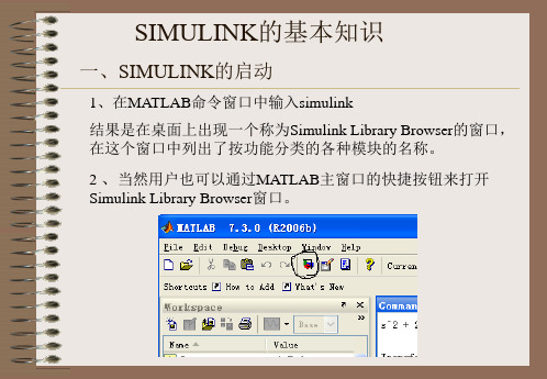
一、SIMULINK的启动
1、在MATLAB命令窗口中输入simulink 结果是在桌面上出现一个称为Simulink Library Browser的窗口, 在这个窗口中列出了按功能分类的各种模块的名称。 2 、当然用户也可以通过MATLAB主窗口的快捷按钮来打开 Simulink Library Browser窗口。
matlab simulink模型搭建方法
matlab simulink模型搭建方法Matlab Simulink是一个强大的多领域仿真和模型搭建环境,广泛应用于控制系统、信号处理、通信系统等多个领域。
本文将详细介绍Matlab Simulink模型搭建的方法,帮助您快速掌握这一技能。
一、Simulink基础操作1.启动Simulink:在Matlab命令窗口输入“simulink”,然后按回车键,即可启动Simulink。
2.创建新模型:在Simulink开始页面,点击“新建模型”按钮,或在菜单栏中选择“文件”→“新建”→“模型”,创建一个空白模型。
3.添加模块:在Simulink库浏览器中,找到所需的模块,将其拖拽到模型窗口中。
4.连接模块:将鼠标光标放在一个模块的输出端口上,按住鼠标左键并拖拽到另一个模块的输入端口,松开鼠标左键,完成模块间的连接。
5.参数设置:双击模型窗口中的模块,可以设置模块的参数。
6.模型仿真:在模型窗口中,点击工具栏上的“开始仿真”按钮,或选择“仿真”→“开始仿真”进行模型仿真。
二、常见模块介绍1.源模块:用于生成信号,如Step、Ramp、Sine Wave等。
2.转换模块:用于信号转换和处理,如Gain、Sum、Product、Scope 等。
3.控制模块:用于实现控制算法,如PID Controller、State-Space等。
4.建模模块:用于构建物理系统的数学模型,如Transfer Fcn、State-Space等。
5.仿真模块:用于设置仿真参数,如Stop Time、Solver Options等。
三、模型搭建实例以下以一个简单的线性系统为例,介绍Simulink模型搭建过程。
1.打开Simulink,创建一个空白模型。
2.在库浏览器中找到以下模块,并将其添加到模型窗口中:- Sine Wave(正弦波信号源)- Transfer Fcn(传递函数模块)- Scope(示波器模块)3.连接模块:- 将Sine Wave的输出端口连接到Transfer Fcn的输入端口。
MATLAB-SIMULINK讲解完整版
图3-5 模块的基本操作示例
、按键 、按键 和按键 。
(5) 窗口切换类:包括 6 个按键,分别是按键 、按键
、按键 、按键 、按键 和按键 。
工具栏中各个工具图标及其功能说明见附录 B。
3.2 SIMULINK的基本操作 3.2.1 模块及信号线的基本操作
1. 模块的基本操作 模块是系统模型中最基本的元素,不同模块代表了不同 的功能。各模块的大小、放置方向、标签、属性等都是可以 设置调整的。表3-1列出了SIMULINK中模块基本操作方法 的简单描述。
善模型的外观
标左键
可改变折线的走向, 选中目标节点,按住鼠标左键,拖曳到目标位置,松开鼠
改善模型的外观
标左键
从一个节点引出多 条信号线,应用于不同 目的
方法 1:先按住“Ctrl”键,再选中信号引出点,按住鼠标 左键,拖曳到下级目标模块的信号输入端,松开鼠标左键;
方法 2:先选中信号引出线,然后在信号引出点按住鼠标 右键,拖曳到下级目标模块的信号输入端,松开鼠标右键
如图3-6所示,在模型中加入注释文字,使模型更具可 读性。
图3-6 添加注释文字示例 (a) 未加注释文字;(b) 加入注释文字
3.2.3 子系统的建立与封装 1. 子系统的建立 一般而言,电力系统仿真模型都比较复杂,规模很大,
包含了数量可观的各种模块。如果这些模块都直接显示在 SIMULINK仿真平台窗口中,将显得拥挤、杂乱,不利于用 户建模和分析。可以把实现同一种功能或几种功能的多个模 块组合成一个子系统,从而简化模型,其效果如同其它高级 语言中的子程序和函数功能。
如何使用MATLABSimulink进行系统建模
如何使用MATLABSimulink进行系统建模如何使用MATLAB Simulink进行系统建模第一章:MATLAB Simulink简介Matlab Simulink是一款基于MATLAB的工程工具软件,用于进行系统建模和仿真。
它提供了一种直观的图形化方法,使工程师能够轻松地建立和模拟复杂的系统。
Simulink支持各种工程学科,包括电气、机械、控制和通信等领域。
本章将简要介绍MATLAB Simulink的基本概念和主要功能。
1.1 Simulink的基本概念Simulink使用图形化的方式进行系统建模,系统模型由各种元件和信号线组成。
元件表示系统的各个组成部分,信号线表示元件之间的数据传输。
1.2 Simulink的主要功能Simulink具有以下主要功能:- 系统建模:通过拖拽和连接元件,可以快速搭建系统模型。
- 仿真和调试:使用仿真器可以对系统模型进行实时仿真,并进行调试和分析。
- 自动代码生成:Simulink可以自动生成C、C++、Verilog等编程语言的代码,可用于系统的实现和验证。
第二章:Simulink建模基础在本章中,我们将详细介绍如何使用Simulink进行系统建模的基础知识和技巧。
2.1 模型创建在Simulink中,可以通过选择“File -> New Model”来创建一个新的模型。
在模型中,可以使用工具栏上的元件库来选择需要的元件,然后将其拖拽到模型中。
2.2 连接元件在模型中,元件之间的连接通常使用信号线来表示。
可以通过鼠标点击元件输出端口和输入端口的方式来建立连接。
可以使用线段工具来绘制信号线,也可以使用Ctrl + 鼠标点击来删除信号线。
2.3 参数设置在建模过程中,可以通过双击元件来设置各个元件的参数。
每个元件都有各自的参数面板,可以根据具体需求进行设置。
第三章:Simulink高级建模技巧在本章中,我们将介绍一些进阶的Simulink建模技巧,如子系统的使用、模型的分层和复用等。
MATLAB语言及应用-10 simulink入门
首先启动MATLAB软件,然后再启动Simulink。用户可以 单击MATLAB主界面工具栏的按钮,或在命令行窗口输入: simulink,来启动Simulink。
在MATLAB的命令行输入:help simulink,来查看Simulink 命令行下的函数。
在命令行输入:demo simulink,将会打开MATLAB的帮助 系统,并显示Simulink的例子程序。
10.2.2 选择模块
分析待仿真系统,确定待建模型的功能需求和结构。
打开Simulink的库浏览器窗口。然后单击Simulink库浏览 器窗口工具栏上的New按钮,新建模型文件,并保存为 exam.mdl。
仿真技术的主要用途有如下几点: (1) 优化系统设计。在实际系统建立以前,通过改变仿真模型 结构和调整系统参数来优化系统设计。如控制系统、数字信号 处理系统的设计经常要靠仿真来优化系统性能。 (2) 系统故障再现,发现故障原因。实际系统故障的再现必然 会带来某种危害性,这样做是不安全的和不经济的,利用仿真 来再现系统故障则是安全的和经济的。 (3) 验证系统设计的正确性。 (4) 对系统或其子系统进行性能评价和分析。多为物理仿真, 如飞机的疲劳试验。 (5) 训练系统操作员。常见于各种模拟器,如飞行模拟器、坦 克模拟器等。 (6) 为管理决策和技术决策提供支持。
通过观察可以发现:纵坐标的适当范围大致在[-0.06,0.06],仿 真时间取[0,5]即可
(9)示波器纵坐标设置 用鼠标右键单击示波器的黑色显示屏,在弹出菜单中选择 Axis Properties,引出纵坐标设置对话框。
控制系统计算机仿真(内蒙古工业大学)MATLAB基础第6章 SIMULINK仿真基础
Transfer-Fcn:线性传递函数模型
Transport Delay:输入信号延时一个固定时间再输出 Variable Transport Delay:输入信号延时一个可变时间再输出 Zero-Pole:以零极点表示的传递函数模型
2、Discontinuities (非线性模块) Backlash:死区间隙 Coulomb &Viscous Friction:库仑粘滞摩擦信号 Dead Zone:死区信号 Hit Crossing:将信号与特定的偏移值比较 Quantizer;量化器 Rate Limiter;信号上升、下降速率控制器 Relay:滞环比较器,限制输出值在某一范围内变化。 Saturation:饱和信号,让输出超过某一值时能够饱和。
第一节 SIMULINK简介 一、什么是SIMULINK
SIMULINK是MATLAB软件的扩展,它是实现动态系 统建模和仿真的一个软件包,它与MATLAB语言的主要 区别在于,其与用户交互接口是基于Windows的模型化 图形输入。
所谓模型化图形输入是指SIMULINK提供了一些按功 能分类的基本的系统模块,用户只需知道这些模块的输 入输出及模块的功能,而不必考察模块内部是如何实现 的,通过对这些基本模块的调用,再将它们连接起来就 可以构成所需要的系统模型(以.mdl文件进行存取), 进而进行仿真与分析。
三、SIMULINK的公共模块库
SIMILINK模块库按功能进行分类,包括以下子库: Continuous(连续模块) disontinuous (非线性模块) Discrete(离散模块) look up tables(查询表模块)
Math operations(数学模块)Model verification(模型检测) Model-wide Utilities(模型扩展功能模块) Ports&Systems(端口和子系统模块) Signal attributes(信号描述模块)
- 1、下载文档前请自行甄别文档内容的完整性,平台不提供额外的编辑、内容补充、找答案等附加服务。
- 2、"仅部分预览"的文档,不可在线预览部分如存在完整性等问题,可反馈申请退款(可完整预览的文档不适用该条件!)。
- 3、如文档侵犯您的权益,请联系客服反馈,我们会尽快为您处理(人工客服工作时间:9:00-18:30)。
MATLAB-Simulink基础§1Simulink简介Simulink是一个用来对动态系统进行建模、仿真和分析的软件包,它支持连续、离散及两者混合的线性和非线性系统,也支持具有多种采样频率的系统。
在Simulink环境中,利用鼠标就可以在模型窗口中直观地“画”出系统模型,然后直接进行仿真。
它为用户提供了方框图进行建模的图形接口,采用这种结构画模型就像你用手和纸来画一样容易。
它与传统的仿真软件包微分方程和差分方程建模相比,具有更直观、方便、灵活的优点。
Simulink包含有Sink(输出方式)、Source(输入源)、Linear(线性环节)、Nonlinear(非线性环节)、Connection(连接与接口)和E某tra(其他环节)等子模型库,而且每个子模型库中包含有相应的功能模块,用户也可以定制和创建自己的模块。
用Simulink创建的模型可以具有递阶结构,因此用户可以采用从上到下或从下到上的结构创建模型。
用户可以从最高级开始观看模型,然后用鼠标双击其中的子系统模块,来查看其下一级的内容,以此类推,从而可以看到整个模型的细节,帮助用户理解模型的结构和各模块之间的相互关系。
在定义完一个模型后,用户可以通过Simulink的菜单或MATLAB的命令窗口键入命令来对它进行仿真。
菜单方式对于交互工作非常方便,而命令行方式对于运行一大类仿真非常有用。
采用Scope模块和其他的画图模块,在仿真进行的同时,就可观看到仿真结果。
除此之外,用户还可以在改变参数后迅速观看系统中发生的变化情况。
仿真的结果还可以存放到MATLAB的工作空间里做事后处理。
模型分析工具包括线性化和平衡点分析工具、MATLAB的许多基本工具箱及MATLAB的应用工具箱。
由于MATLAB和Simulink是集成在一起的,因此用户可以在这两种环境下对自己的模型进行仿真、分析和修改。
Simulink具有非常高的开放性,提倡将模型通过框图表示出来,或者将已有的模型添加组合到一起,或者将自己创建的模块添加到模型当中。
Simulink具有较高的交互性,允许随意修改模块参数,并且可以直接无缝地使用MATLAB的所有分析工具。
对最后得到的结果可进行分析,并能够将结果可视化显示。
Simulink非常实用,应用领域很广,可使用的领域包括航空航天、电子、力学、数学、通信、影视和控制等。
世界各地的工程师都在利用它来对实际问题进行建模、分析和解决。
§2Simulink的基本操作2.1Simulink的运行运行Simulink有三种方式:在MATLAB的命令窗口直接键入“Simulink”并回车;单击MATLAB工具条上的Simulink图标;在MATLAB菜单上选File→New→Model。
运行后会显示图2.1所示的Simulink模块库浏览器,单击工具条左边建立新模型的快捷方式,则显示如图2.2所示的新建模型窗口,在模型窗口中用户便可通过选择模块库中的仿真模块,建立自己的仿真模型,并进行动态仿真。
图2.1Simulink模块库浏览器图2.2新建模型窗口2.2常用的标准模块附录C以表格的形式给出Simulink几个基本模块库中的模块功能简介,表格中的模块名和模块库中的模块图标下的名称一致。
打开模块库(图标)窗口的方法非常简单,以连续系统模块库(continuou)为例,在Simulink模块库浏览窗口中选中Simulink,然后单击Simulink旁边的小加号或者双击鼠标左键,这时就会出现如图2.3所示Simulink基本库窗口,并选择Continuou模块库的图标双击即可进入如图2.4所示的连续系统模块库,可选择相应的模块图标拖至编辑窗口即可。
2图2.3Simulink模型库窗口图2.4continuou模块库2.3模块的操作图2.5选取模块1、模块的选取当选取单个模块时,只要用鼠标在模块上单击即可,此时模块的角上出现黑色小方块。
选取多个模块时,选取拖拽鼠标的方式把要选择的模块全部包围即可,若所有被选取的模块都出现小黑方块,则表示模块被选中,如图2.5所示。
2、模块的复制、剪切、删除、移动应用【Edit】│【copy】/【cut】/【pate】/【clear】可对选取的模块进行复制,剪切,粘贴,删除等操3作,如果要在同一窗口移动模块,则在模块选中的基础上,用鼠标进行拖拽并放在合适的位置。
3、模块的连接(1)连接两个模块:从一个模块的输出端连到另一个模块的输入端。
如果两个模块不在同一水平线上,连线是折线,若用斜线表示则需在连接时按住【Shift】。
(2)在连线之间插入:把模块用鼠标拖到连线上,然后释放鼠标即可。
(3)连线的分支:当我们需要把一个信号输送给不同的模块时,连线要采用分支结构,其操作步骤是:先连好一条线,把鼠标移到支线的起点,并按下【Ctrl】,再将鼠标拖至目标模块的输入端即可。
4、模块参数的设置Simulink中几乎所有模块的参数(Parameter)都允许用户进行设置,只要双击要设置的模块或在模块上按鼠标右键并在弹出的菜单中选择【BlockParameter】就会显示参数设置对话框。
例2.1已知单位负反馈二阶系统的开环传递函数为试绘制单位阶跃响应的Simulink结构图。
解:1、利用Simulink的Library窗口中的【File】|【New】,打开一个新的工作空间;2、分别从信号源库(Soure)、输出方式库(Sink)、数学运算库(Math)、连续系统库(Continuou)中,用鼠标把阶跃信号发生器(Step)、示波器(Scope)、传递函数(TranferFcn)、相加器(Sum)四个标准功能模块选中,并将其拖至工作平台;3、按要求先将前向通道连接好,然后把相加器(Sum)的另一个端口与传递函数和示波器间的线段相连,形成闭环反馈;4、双击阶跃信号发生器,打开其属性设置对话框,并将其设置为单位阶跃信号,如图2.6所示,同理,将相加器设置为“+-”,使传递函数的Numerator设置为“[10]”,Denominator设置为“[14.470]”;图2.6模块参数设置对话框5、绘制成功后,如图2.7所示,并命名后存盘。
图2.7二阶系统Simulink结构图5、模块外形的调整(1)改变模块的大小:选定模块,用鼠标点住其周围的四个黑方块中的任意一个拖动,这时会出现一个虚线的矩形表示新模块的位置,到需要的位置后释放鼠标即可。
(2)调整模块的方向:选定模块,选择菜单【Formt】|【RotateBlock】使模块旋转90°,【FlipBlock】4使模块旋转180°。
(3)给模块加阴影:选定模块,选择菜单【Formt】|【ShowDropShadow】使模块产生阴影效果。
6、模块名的处理(1)模块名的显示与消隐:选定模块,选择菜单【Format】|【FilpName】使模块名被隐藏,同时【ShowName】会使隐藏的模块名显示出来。
(2)修改模块名:用鼠标左键单击模块名的区域,使光标处于编辑状态,此时便可对模块名进行任意的修改。
同时选定模块,选择菜单【Format】|【Font】可弹出字体对话框,用户可对模块名和模块图标中的字体进行设置。
例2.2将图2.7所示的结构图进行模块处理。
解:1.对模块名进行修改,如单击传递函数模块标题“TranferFcn”,将其原字符删除,并输入汉字“传递函数”,同理将其他模块也改为汉字标题;2.将相加器的标题移至其顶部;3.选中“传递函数”模块,并选择菜单【Formt】|【ShowDropShadow】并将其设置为阴影;4.将模块全部选中,选择菜单【Format】|【Font】通过字体对话框将所有字体设置为“宋体”,如图2.8所示。
图2.8二阶系统模型§3系统仿真及参数设置在Simulink中建立起系统模型框图后,运行菜单【Simulation】|【Start】就可以用Simulink对模型进行动态仿真。
一般在仿真运行前需要对仿真参数进行设置,运行菜单【Simulation】|【Parameter】完成设置,如图3.1所示。
图3.1仿真参数设置对话框53.1算法设置(1)算法类型设置仿真的主要过程一般是求解常微分方程组,【Solveroption】|【Type】用来选择仿真算法的类型是变化的还是固定的。
变步长解法可以在仿真过程中根据要求调整运算步长,在采用变步长解法时,应该先指定一个容许误差限(【Relativetolerance】或【Abolutetolerance】),使得当误差超过误差限时自动修正仿真步长,【Ma某tepize】用于设置最大步长,在缺省情况下为“auto”,并按下式计算最大步长:最大步长=(终止时间-起始时间)/50。
(2)仿真算法设置离散模型:对变步长和定步长解法均采用dicrete(nocontinuoutate)。
连续模型:可采用变步长和定步长解法。
变步长解法有:ode45、ode23、ode113、ode15、ode23、ode23t,ode23tode45:四阶/五阶Runge-Kutta算法,属单步解法;ode23:二阶/三阶Runge-Kutta算法,属单步解法;ode113:可变阶次的Adam-Bahforth-MoultonPECE算法,属于多步解法;ode15:可变阶次的数值微分公式算法,属于多步解法;ode23:基于修正的Roenbrock公式,属单步解法。
定步长解法有:ode4、ode5、ode3、ode2、ode1ode5:定步长的ode45解法;ode4:四阶Runge-Kutta算法;ode3:定步长ode23算法;ode2:Henu方法,即改进的欧拉法。
ode1:欧拉法。
3设置输出选项图3.2二阶系统的仿真曲线对同样的信号,选择不同的输出选项,则得到输出设备上的信号是不完全一样的。
要根据需要选择合适的输出选项以达到满意的输出效果。
6对于例2.2,首先运行菜单【Simulation】|【Parameter】,进行系统的仿真参数设置,如仿真时间为2秒,仿真算法选择定步长的四阶龙格—库塔法,然后运行菜单【Simulation】|【Start】进行系统仿真,最后双击示波器,得到系统的仿真曲线如图3.2所示。
3.2工作空间设置工作空间设置(WorkpaceI/O)窗口如图3.3所示,可以设置Simulink和当前工作空间的数据输入、输出。
通过设置,可以从工作空间输入数据、初始化状态模块,也可以把仿真结果、状态变量、时间数据保存到当前工作空间。
图3.3设置WorkpaceI/O窗口1、从工作空间读入数据(Loadfromworkpace)Simulink通过设置模型的输入端口,实现在仿真过程中从工作空间读入数据,常用的输入端口模块为信号与系统模块库(Signal&Sytem)中的In1模块,其参数设置如图3.4所示。