Algorithm to estimate the Hurst exponent of high-dimensional fractals

合集下载

Analyzing the Scalability of Algorithms

Analyzing the Scalability ofAlgorithmsAlgorithms are essential tools used in various fields such as computer science, data analysis, and machine learning. The scalability of algorithms refers to their ability to handle increasing amounts of data or growing computational demands efficiently without compromising performance. In this article, we will delve into the concept of scalability of algorithms and discuss various factors that influence it.One of the key factors that affect the scalability of algorithms is the input size. As the amount of data increases, the algorithm should be able to process it within a reasonable time frame. The efficiency of an algorithm can be measured in terms of its time complexity, which describes how the running time of the algorithm grows with the size of the input. Algorithms with a lower time complexity are more scalable as they can handle larger inputs without a significant increase in processing time.Another important factor to consider is the space complexity of an algorithm. Space complexity refers to the amount of memory or storage space required by the algorithm to solve a problem. As the input size grows, the algorithm should not consume an excessive amount of memory, as this can lead to performance degradation or even failure to complete the computation. Algorithms with lower space complexity are more scalable as they can operate efficiently even with limited memory resources.Moreover, the structure and design of an algorithm can greatly impact its scalability. Algorithms that are well-structured and modularized are easier to scale as they can be optimized or parallelized to improve performance. Additionally, the choice of data structures and algorithms used within the main algorithm can influence its scalability. For example, utilizing efficient data structures such as arrays or hash tables can improve the scalability of the algorithm by reducing the time and space required for processing.Furthermore, the scalability of algorithms can also be affected by external factors such as hardware limitations or network constraints. Algorithms that are designed towork in a distributed system or parallel computing environment are more scalable as they can distribute the workload across multiple processing units. However, algorithms that rely on a single processor or have high communication overhead may not scale well when faced with increasing computational demands.In conclusion, analyzing the scalability of algorithms is crucial for ensuring optimal performance in handling large datasets or complex computational tasks. Understanding the factors that influence scalability, such as time complexity, space complexity, algorithm structure, and external constraints, can help developers and researchers design and implement scalable algorithms. By considering these factors and optimizing the algorithm accordingly, we can improve efficiency, reduce resource consumption, and achieve better performance in various applications.。

全球气候变化Global temperature change

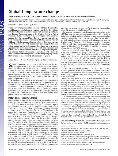
Global temperature changeJames Hansen*†‡,Makiko Sato*†,Reto Ruedy*§,Ken Lo*§,David W.Lea ¶,and Martin Medina-Elizade ¶*National Aeronautics and Space Administration Goddard Institute for Space Studies,†Columbia University Earth Institute,and §Sigma Space Partners,Inc.,2880Broadway,New York,NY 10025;and ¶Department of Earth Science,University of California,Santa Barbara,CA 93106Contributed by James Hansen,July 31,2006Global surface temperature has increased Ϸ0.2°C per decade in the past 30years,similar to the warming rate predicted in the 1980s in initial global climate model simulations with transient greenhouse gas changes.Warming is larger in the Western Equatorial Paciﬁc than in the Eastern Equatorial Paciﬁc over the past century,and we suggest that the increased West–East temperature gradient may have increased the likelihood of strong El Niños,such as those of 1983and parison of measured sea surface temperatures in the Western Paciﬁc with paleoclimate data suggests that this critical ocean region,and probably the planet as a whole,is approximately as warm now as at the Holocene maximum and within Ϸ1°C of the maximum temperature of the past million years.We conclude that global warming of more than Ϸ1°C,relative to 2000,will constitute ‘‘dangerous’’climate change as judged from likely effects on sea level and extermination of species.climate change ͉El Niños ͉global warming ͉sea level ͉species extinctionsGlobal temperature is a popular metric for summarizing the state of global climate.Climate effects are felt locally,but the global distribution of climate response to many global climate forcings is reasonably congruent in climate models (1),suggesting that the global metric is surprisingly useful.We will argue further,consistent with earlier discussion (2,3),that measurements in the Western Pacific and Indian Oceans provide a good indication of global temperature change.We first update our analysis of surface temperature change based on instrumental data and compare observed temperature change with predictions of global climate change made in the 1980s.We then examine current temperature anomalies in the tropical Pacific Ocean and discuss their possible significance.Finally,we compare paleoclimate and recent data,using the Earth’s history to estimate the magnitude of global warming that is likely to constitute dan-gerous human-made climate change.Modern Global Temperature ChangeGlobal surface temperature in more than a century of instrumental data is recorded in the Goddard Institute for Space Studies analysis for 2005.Our analysis,summarized in Fig.1,uses documented procedures for data over land (4),satellite measurements of sea surface temperature (SST)since 1982(5),and a ship-based analysis for earlier years (6).Estimated 2␴error (95%confidence)in comparing nearby years of global temperature (Fig.1A ),such as 1998and 2005,decreases from 0.1°C at the beginning of the 20th century to 0.05°C in recent decades (4).Error sources include incomplete station coverage,quantified by sampling a model-generated data set with realistic variability at actual station loca-tions (7),and partly subjective estimates of data quality problems (8).The estimated uncertainty of global mean temperature implies that we can only state that 2005was probably the warmest year.The map of temperature anomalies for the first half-decade of the 21st century (Fig.1B ),relative to 1951–1980climatology,shows that current warmth is nearly ubiquitous,generally larger over land than over ocean,and largest at high latitudes in the Northern Hemi-sphere.Our ranking of 2005as the warmest year depends on the positive polar anomalies,especially the unusual Arctic warmth.In calculating the global mean,we give full weight to all regions based on area.Meteorological stations are sparse in the Arctic,but the estimated strong warm anomaly there in 2005is consistent withrecord low sea ice concentration and Arctic temperature anomalies inferred from infrared satellite data (9).Our analysis includes estimated temperature anomalies up to 1,200km from the nearest measurement station (7).Resulting spatial extrapolations and interpolations of temperature anomalies usually are meaningful for seasonal and longer time scales at middle and high latitudes,where the spatial scale of anomalies is set by Rossby waves (7).Thus,we believe that the unusual Arctic warmth of 2005is real.Other characteristics of our analysis method are summarized in Supporting Text ,which is published as supporting information on the PNAS web site.Independent analysis by the National Climate Data Center ( ͞oa ͞climate ͞research ͞2005͞ann ͞global.html),using a ‘‘teleconnection’’approach to fill in data sparse regions,also finds 2005to be the warmest year.The joint analysis of the University of East Anglia and the Hadley Centre ( ͞research ͞hadleycentre ͞obsdata ͞globaltemperature.html)also yields high global tem-perature for 2005,but a few hundredths of a degree cooler than in 1998.Record,or near record,warmth in 2005is notable,because global temperature did not receive a boost from an El Niño in 2005.The temperature in 1998,on the contrary,was lifted 0.2°C above the trend line by a ‘‘super El Niño’’(see below),the strongest El Niño of the past century.Global warming is now 0.6°C in the past three decades and 0.8°C in the past century.It is no longer correct to say ‘‘most global warming occurred before 1940.’’A better summary is:slow global warming,with large fluctuations,over the century up to 1975,followed by rapid warming at a rate Ϸ0.2°C per decade.Global warming was Ϸ0.7°C between the late 19th century (the earliest time at which global mean temperature can be accurately defined)and 2000,and continued warming in the first half decade of the 21st century is consistent with the recent rate of ϩ0.2°C per decade.The conclusion that global warming is a real climate change,not an artifact due to measurements in urban areas,is confirmed by surface temperature change inferred from borehole temperature profiles at remote locations,the rate of retreat of alpine glaciers around the world,and progressively earlier breakup of ice on rivers and lakes (10).The geographical distribution of warming (Fig.1B )provides further proof of real climate rgest warming is in remote regions including high latitudes.Warming occurs over ocean areas,far from direct human effects,with warming over ocean less than over land,an expected result for a forced climate change because of the ocean’s great thermal inertia.Early Climate Change Predictions.Manabe and Wetherald (11)madethe first global climate model (GCM)calculations of warming dueAuthor contributions:D.W.L.and M.M.-E.contributed data;J.H.,M.S.,R.R.,K.L.,D.W.L.,and M.M.-E.analyzed data;and J.H.wrote the paper.The authors declare no conﬂict of interest.Freely available online through the PNAS open access option.Abbreviations:SST,sea surface temperature;GHG,greenhouse gas;EEP,Eastern Equatorial Paciﬁc;WEP,Western Equatorial Paciﬁc;DAI,dangerous antrhopogenic interference;BAU,business as usual;AS,alternative scenario;BC,black carbon.‡Towhom correspondence should be addressed:E-mail:jhansen@.©2006by The National Academy of Sciences of the USA14288–14293͉PNAS ͉September 26,2006͉vol.103͉no.39 ͞cgi ͞doi ͞10.1073͞pnas.0606291103to instant doubling of atmospheric CO 2.The first GCM calculations with transient greenhouse gas (GHG)amounts,allowing compar-ison with observations,were those of Hansen et al.(12).It has been asserted that these calculations,presented in congressional testi-mony in 1988(13),turned out to be ‘‘wrong by 300%’’(14).That assertion,posited in a popular novel,warrants assessment because the author’s views on global warming have been welcomed in testimony to the United States Senate (15)and in a meeting with the President of the United States (16),at a time when the Earth may be nearing a point of dangerous human-made interference with climate (17).The congressional testimony in 1988(13)included a graph (Fig.2)of simulated global temperature for three scenarios (A,B,and C)and maps of simulated temperature change for scenario B.The three scenarios were used to bracket likely possibilities.Scenario A was described as ‘‘on the high side of reality,’’because it assumed rapid exponential growth of GHGs and it included no large volcanic eruptions during the next half century.Scenario C was described as ‘‘a more drastic curtailment of emissions than has generally been imagined,’’specifically GHGs were assumed to stop increasing after 2000.Intermediate scenario B was described as ‘‘the most plausi-ble.’’Scenario B has continued moderate increase in the rate of GHG emissions and includes three large volcanic eruptions sprin-kled through the 50-year period after 1988,one of them in the 1990s.Real-world GHG climate forcing (17)so far has followed a course closest to scenario B.The real world even had one large volcanic eruption in the 1990s,Mount Pinatubo in 1991,whereas scenario B placed a volcano in 1995.Fig.2compares simulations and observations.The red curve,as in ref.12,is the updated Goddard Institute for Space Studies observational analysis based on meteorological stations.The black curve is the land–ocean global temperature index from Fig.1,which uses SST changes for ocean areas (5,6).The land–ocean temper-ature has more complete coverage of ocean areas and yields slightly smaller long-term temperature change,because warming on aver-age is less over ocean than over land (Fig.1B ).Temperature change from climate models,including that re-ported in 1988(12),usually refers to temperature of surface air over both land and ocean.Surface air temperature change in a warming climate is slightly larger than the SST change (4),especially in regions of sea ice.Therefore,the best temperature observation for comparison with climate models probably falls between the mete-orological station surface air analysis and the land–ocean temper-ature index.Observed warming (Fig.2)is comparable to that simulated for scenarios B and C,and smaller than that for scenario A.Following refs.18and 14,let us assess ‘‘predictions’’by comparing simulated and observed temperature change from 1988to the most recent year.Modeled 1988–2005temperature changes are 0.59,0.33,and 0.40°C,respectively,for scenarios A,B,and C.Observed temper-ature change is 0.32°C and 0.36°C for the land–ocean index and meteorological station analyses,respectively.Warming rates in the model are 0.35,0.19,and 0.24°C per decade for scenarios A,B.and C,and 0.19and 0.21°C per decade for the observational analyses.Forcings in scenarios B and C are nearly the same up to 2000,so the different responses provide one measure of unforced variability in the model.Because of this chaotic variability,a 17-year period is too brief for precise assessment of model predictions,but distinction among scenarios and comparison with the real world will become clearer within a decade.Close agreement of observed temperature change with simula-tions for the most realistic climate forcing (scenario B)is accidental,given the large unforced variability in both model and real world.Indeed,moderate overestimate of global warming is likely because the sensitivity of the model used (12),4.2°C for doubled CO 2,is larger than our current estimate for actual climate sensitivity,which is 3Ϯ1°C for doubled CO 2,based mainly on paleoclimate data (17).More complete analyses should include other climate forcingsandFig.1.Surface temperature anomalies relative to 1951–1980from surface air measurements at meteorological stations and ship and satellite SST measurements.(A )Global annual mean anomalies.(B )Temperature anomaly for the ﬁrst half decade of the 21stcentury.Annual Mean Global Temperature Change: ΔT s (°C)Fig.2.Global surface temperature computed for scenarios A,B,and C (12),compared with two analyses of observational data.The 0.5°C and 1°C tempera-ture levels,relative to 1951–1980,were estimated (12)to be maximum global temperatures in the Holocene and the prior interglacial period,respectively.Hansen et al.PNAS ͉September 26,2006͉vol.103͉no.39͉14289E N V I R O N M E N T A L S C I E N C EScover longer periods.Nevertheless,it is apparent that the first transient climate simulations (12)proved to be quite accurate,certainly not ‘‘wrong by 300%’’(14).The assertion of 300%error may have been based on an earlier arbitrary comparison of 1988–1997observed temperature change with only scenario A (18).Observed warming was slight in that 9-year period,which is too brief for meaningful comparison.Super El Niños.The 1983and 1998El Niños were successivelylabeled ‘‘El Niño of the century,’’because the warming in the Eastern Equatorial Pacific (EEP)was unprecedented in 100years (Fig.3).We suggest that warming of the Western Equatorial Pacific (WEP),and the absence of comparable warming in the EEP,has increased the likelihood of such ‘‘super El Niños.’’In the ‘‘normal’’(La Niña)phase of El Niño Southern Oscillation the east-to-west trade winds push warm equatorial surface water to the west such that the warmest SSTs are located in the WEP near Indonesia.In this normal state,the thermocline is shallow in the EEP,where upwelling of cold deep water occurs,and deep in the WEP (figure 2of ref.20).Associated with this tropical SST gradient is a longitudinal circulation pattern in the atmosphere,the Walker cell,with rising air and heavy rainfall in the WEP and sinking air and drier conditions in the EEP.The Walker circulation enhances upwelling of cold water in the East Pacific,causing a powerful positive feedback,the Bjerknes (21)feedback,which tends to maintain the La Niña phase,as the SST gradient and resulting higher pressure in the EEP support east-to-west trade winds.This normal state is occasionally upset when,by chance,the east-to-west trade winds slacken,allowing warm water piled up in the west to slosh back toward South America.If the fluctuation is large enough,the Walker circulation breaks down and the Bjerknes feedback loses power.As the east-to-west winds weaken,the Bjerknes feedback works in reverse,and warm waters move more strongly toward South America,reducing the thermocline tilt and cutting off upwelling of cold water along the South American coast.In this way,a classical El Niño is born.Theory does not provide a clear answer about the effect of global warming on El Niños (19,20).Most climate models yield either a tendency toward a more El Niño-like state or no clear change (22).It has been hypothesized that,during the early Pliocene,when the Earth was 3°C warmer than today,a permanent El Niño condition existed (23).We suggest,on empirical grounds,that a near-term global warming effect is an increased likelihood of strong El Niños.Fig.1B shows an absence of warming in recent years relative to 1951–1980in the equatorial upwelling region off the coast of South America.This is also true relative to the earliest period of SST data,1870–1900(Fig.3A ).Fig.7,which is published as supporting information on the PNAS web site,finds a similar result for lineartrends of SSTs.The trend of temperature minima in the East Pacific,more relevant for our purpose,also shows no equatorial warming in the East Pacific.The absence of warming in the EEP suggests that upwelling water there is not yet affected much by global warming.Warming in the WEP,on the other hand,is 0.5–1°C (Fig.3).We suggest that increased temperature difference between the near-equatorial WEP and EEP allows the possibility of increased temperature swing from a La Niña phase to El Niño,and that this is a consequence of global warming affecting the WEP surface sooner than it affects the deeper ocean.Fig.3B compares SST anomalies (12-month running means)in the WEP and EEP at sites (marked by circles in Fig.3A )of paleoclimate data discussed below.Absolute temperatures at these sites are provided in Fig.8,which is published as supporting information on the PNAS web site.Even though these sites do not have the largest warming in the WEP or largest cooling in the EEP,Fig.3B reveals warming of the WEP relative to the EEP [135-year changes,based on linear trends,are ϩ0.27°C (WEP)and Ϫ0.01°C (EEP)].The 1983and 1998El Niños in Fig.3B are notably stronger than earlier El Niños.This may be partly an artifact of sparse early data or the location of data sites,e.g.,the late 1870s El Niño is relatively stronger if averages are taken over Niño 3or a 5°ϫ10°box.Nevertheless,‘‘super El Niños’’clearly were more abundant in the last quarter of the 20th century than earlier in the century.Global warming is expected to slow the mean tropical circulation (24–26),including the Walker cell.Sea level pressure data suggest a slowdown of the longitudinal wind by Ϸ3.5%in the past century (26).A relaxed longitudinal wind should reduce the WEP–EEP temperature difference on the broad latitudinal scale (Ϸ10°N to 15°S)of the atmospheric Walker cell.Observed SST anomalies are consistent with this expectation,because the cooling in the EEP relative to WEP decreases at latitudes away from the narrower region strongly affected by upwelling off the coast of Peru (Fig.3A ).Averaged over 10°N to 15°S,observed warming is as great in the EEP as in the WEP (see also Fig.7).We make no suggestion about changes of El Niño frequency,and we note that an abnormally warm WEP does not assure a strong El Niño.The origin and nature of El Niños is affected by chaotic ocean and atmosphere variations,the season of the driving anomaly,the state of the thermocline,and other factors,assuring that there will always be great variability of strength among El Niños.Will increased contrast between near-equatorial WEP and EEP SSTs be maintained or even increase with more global warming?The WEP should respond relatively rapidly to increasing GHGs.In the EEP,to the extent that upwelling water has not been exposed to the surface in recent decades,little warming is expected,andtheBSST Change (°C) from 1870-1900 to 2001-2005Western and Eastern Pacific Temperature Anomalies (°C)parison of SST in West and East Equatorial Paciﬁc Ocean.(A )SST in 2001–2005relative to 1870–1900,from concatenation of two data sets (5,6),as described in the text.(B )SSTs (12-month running means)in WEP and EEP relative to 1870–1900means.14290͉ ͞cgi ͞doi ͞10.1073͞pnas.0606291103Hansen etal.contrast between WEP and EEP may remain large or increase in coming decades.Thus,we suggest that the global warming effect on El Niños is analogous to an inferred global warming effect on tropical storms (27).The effect on frequency of either phenomenon is unclear,depending on many factors,but the intensity of the most powerful events is likely to increase as GHGs increase.In this case,slowing the growth rate of GHGs should diminish the probability of both super El Niños and the most intense tropical storms.Estimating Dangerous Climate ChangeModern vs.Paleo Temperatures.Modern SST measurements (5,6)are compared with proxy paleoclimate temperature (28)in the WEP (Ocean Drilling Program Hole 806B,0°19ЈN,159°22ЈE;site circled in Fig.3A )in Fig.4A .Modern data are from ships and buoys for 1870–1981(6)and later from satellites (5).In concatenation of satellite and ship data,as shown in Fig.8A ,the satellite data are adjusted down slightly so that the 1982–1992mean matches the mean ship data for that period.The paleoclimate SST,based on Mg content of foraminifera shells,provides accuracy to Ϸ1°C (29).Thus we cannot be sure that we have precisely aligned the paleo and modern temperature scales.Accepting paleo and modern temperatures at face value implies a WEP 1870SST in the middle of its Holocene range.Shifting the scale to align the 1870SST with the lowest Holocene value raises the paleo curve by Ϸ0.5°C.Even in that case,the 2001–2005WEPSST is at least as great as any Holocene proxy temperature at that location.Coarse temporal resolution of the Holocene data,Ϸ1,000years,may mask brief warmer excursions,but cores with higher resolution (29)suggest that peak Holocene WEP SSTs were not more than Ϸ1°C warmer than in the late Holocene,before modern warming.It seems safe to assume that the SST will not decline this century,given continued increases of GHGs,so in a practical sense the WEP temperature is at or near its highest level in the Holocene.Fig.5,including WEP data for the past 1.35million years,shows that the current WEP SST is within Ϸ1°C of the warmest intergla-cials in that period.The Tropical Pacific is a primary driver of the global atmosphere and ocean.The tropical Pacific atmosphere–ocean system is the main source of heat transported by both the Pacific and Atlantic Oceans (2).Heat and water vapor fluxes to the atmosphere in the Pacific also have a profound effect on the global atmosphere,as demonstrated by El Niño Southern Oscillation climate variations.As a result,warming of the Pacific has worldwide repercussions.Even distant local effects,such as thinning of ice shelves,are affected on decade-to-century time scales by subtropical Pacific waters that are subducted and mixed with Antarctic Intermediate Water and thus with the Antarctic Circumpolar Current.The WEP exhibits little seasonal or interannual variability of SST,typically Ͻ1°C,so its temperature changes are likely to reflect large scale processes,such as GHG warming,as opposed to small scale processes,such as local upwelling.Thus,record Holocene WEP temperature suggests that global temperature may also be at its highest level.Correlation of local and global temperature change for 1880–2005(Fig.9,which is published as supporting information on the PNAS web site)confirms strong positive correlation of global and WEP temperatures,and an even stronger correlation of global and Indian Ocean temperatures.The Indian Ocean,due to rapid warming in the past 3–4decades,is now warmer than at any time in the Holocene,independent of any plausible shift of the modern temperature scale relative to the paleoclimate data (Fig.4C ).In contrast,the EEP (Fig.4B )and perhaps Central Antarctica (Vostok,Fig.4D )warmed less in the past century and are probably cooler than their Holocene peak values.However,as shown in Figs.1B and 3A ,those are exceptional regions.Most of the world and the global mean have warmed as much as the WEP and Indian Oceans.We infer that global temperature today is probably at or near its highest level in the Holocene.Fig.5shows that recent warming of the WEP has brought its temperature within Ͻ1°C of its maximum in the past million years.There is strong evidence that the WEP SST during the penultimate interglacial period,marine isotope stage (MIS)5e,exceeded the WEP SST in the Holocene by 1–2°C (30,31).This evidence is consistent with data in Figs.4and 5and with our conclusion that the Earth is now within Ϸ1°C of its maximum temperature in the past million years,because recent warming has lifted the current temperature out of the prior Holocenerange.parison of modern surface temperature measurements with paleoclimate proxy data in the WEP (28)(A ),EEP (3,30,31)(B ),Indian Ocean (40)(C ),and Vostok Antarctica (41)(D).Fig.5.Modern sea surface temperatures (5,6)in the WEP compared with paleoclimate proxy data (28).Modern data are the 5-year running mean,while the paleoclimate data has a resolution of the order of 1,000years.Hansen et al.PNAS ͉September 26,2006͉vol.103͉no.39͉14291E N V I R O N M E N T A L S C I E N C ESCriteria for Dangerous Warming.The United Nations FrameworkConvention on Climate Change (www.unfccc.int)has the objective ‘‘to achieve stabilization of GHG concentrations’’at a level pre-venting ‘‘dangerous anthropogenic interference’’(DAI)with cli-mate,but climate change constituting DAI is undefined.We suggest that global temperature is a useful metric to assess proximity to DAI,because,with knowledge of the Earth’s history,global tem-perature can be related to principal dangers that the Earth faces.We propose that two foci in defining DAI should be sea level and extinction of species,because of their potential tragic consequences and practical irreversibility on human time scales.In considering these topics,we find it useful to contrast two distinct scenarios abbreviated as ‘‘business-as-usual’’(BAU)and the ‘‘alternative scenario’’(AS).BAU has growth of climate forcings as in intermediate or strong Intergovernmental Panel on Climate Change scenarios,such as A1B or A2(10).CO 2emissions in BAU scenarios continue to grow at Ϸ2%per year in the first half of this century,and non-CO 2positive forcings such as CH 4,N 2O,O 3,and black carbon (BC)aerosols also continue to grow (10).BAU,with nominal climate sensitivity (3Ϯ1°C for doubled CO 2),yields global warming (above year 2000level)of at least 2–3°C by 2100(10,17).AS has declining CO 2emissions and an absolute decrease of non-CO 2climate forcings,chosen such that,with nominal climate sensitivity,global warming (above year 2000)remains Ͻ1°C.For example,one specific combination of forcings has CO 2peaking at 475ppm in 2100and a decrease of CH 4,O 3,and BC sufficient to balance positive forcing from increase of N 2O and decrease of sulfate aerosols.If CH 4,O 3,and BC do not decrease,the CO 2cap in AS must be lower.Sea level implications of BAU and AS scenarios can be consid-ered in two parts:equilibrium (long-term)sea level change and ice sheet response time.Global warming Ͻ1°C in AS keeps tempera-tures near the peak of the warmest interglacial periods of the past million years.Sea level may have been a few meters higher than today in some of those periods (10).In contrast,sea level was 25–35m higher the last time that the Earth was 2–3°C warmer than today,i.e.,during the Middle Pliocene about three million years ago (32).Ice sheet response time can be investigated from paleoclimate evidence,but inferences are limited by imprecise dating of climate and sea level changes and by the slow pace of weak paleoclimate forcings compared with stronger rapidly increasing human-made forcings.Sea level rise lagged tropical temperature by a few thousand years in some cases (28),but in others,such as Meltwater Pulse 1A Ϸ14,000years ago (33),sea level rise and tropical temperature increase were nearly synchronous.Intergovernmental Panel on Climate Change (10)assumes negligible contribution to 2100sea level change from loss of Greenland and Antarctic ice,but that conclusion is implausible (17,34).BAU warming of 2–3°C would bathe most of Greenland and West Antarctic in melt-water during lengthened melt seasons.Multiple positive feedbacks,in-cluding reduced surface albedo,loss of buttressing ice shelves,dynamical response of ice streams to increased melt-water,and lowered ice surface altitude would assure a large fraction of the equilibrium ice sheet response within a few centuries,at most (34).Sea level rise could be substantial even in the AS,Ϸ1m per century,and cause problems for humanity due to high population in coastal areas (10).However,AS problems would be dwarfed by the disastrous BAU,which could yield sea level rise of several meters per century with eventual rise of tens of meters,enough to transform global coastlines.Extinction of animal and plant species presents a picture anal-ogous to that for sea level.Extinctions are already occurring as a result of various stresses,mostly human-made,including climate change (35).Plant and animal distributions are a reflection of the regional climates to which they are adapted.Thus,plants and animals attempt to migrate in response to climate change,but theirpaths may be blocked by human-constructed obstacles or natural barriers such as coastlines.A study of 1,700biological species (36)found poleward migration of 6km per decade and vertical migration in alpine regions of 6m per decade in the second half of the 20th century,within a factor of two of the average poleward migration rate of surface isotherms (Fig.6A )during 1950–1995.More rapid warming in 1975–2005yields an average isotherm migration rate of 40km per decade in the Northern Hemisphere (Fig.6B ),exceeding known paleoclimate rates of change.Some species are less mobile than others,and ecosystems involve interactions among species,so such rates of climate change,along with habitat loss and fragmentation,new invasive species,and other stresses are expected to have severe impact on species survival (37).The total distance of isotherm migration,as well as migration rate,affects species survival.Extinction is likely if the migration distance exceeds the size of the natural habitat or remaining habitat fragment.Fig.6shows that the 21st century migration distance for a BAU scenario (Ϸ600km)greatly exceeds the average migration distance for the AS (Ϸ100km).It has been estimated (38)that a BAU global warming of 3°C over the 21st century could eliminate a majority (Ϸ60%)of species on the planet.That projection is not inconsistent with mid-century BAU effects in another study (37)or scenario sensitivity of stress effects (35).Moreover,in the Earth’s history several mass extinc-tions of 50–90%of species have accompanied global temperature changes of Ϸ5°C (39).We infer that even AS climate change,which would slow warming to Ͻ0.1°C per decade over the century,would contribute to species loss that is already occurring due to a variety of stresses.However,species loss under BAU has the potential to be truly disastrous,conceivably with a majority of today’s plants and animals headed toward extermination.DiscussionThe pattern of global warming (Fig.1B )has assumed expected characteristics,with high latitude amplification and larger warming over land than over ocean,as GHGs have become the dominant climate forcing in recent decades.This pattern results mainly from the ice–snow albedo feedback and the response times of ocean andland.Fig.6.Poleward migration rate of isotherms in surface observations (A and B )and in climate model simulations (17)for 2000–2100for Intergovernmental Panel on Climate Change scenario A2(10)and an alternative scenario of forcings that keeps global warming after 2000less than 1°C (17)(C and D ).Numbers in upper right are global means excluding the tropical band.14292͉ ͞cgi ͞doi ͞10.1073͞pnas.0606291103Hansen etal.。

The Practice of Approximated Consistency for Knapsack Constraints

The Practice of Approximated Consistency for Knapsack ConstraintsMeinolf SellmannCornell University,Department of Computer Science4130Upson Hall,Ithaca,NY14853,U.S.A.sello@AbstractKnapsack constraints are a key modeling structure in dis-crete optimization and form the core of many real-life prob-lem formulations.Only recently,a cost-basedﬁltering algo-rithm for Knapsack constraints was published that is based onsome previously developed approximation algorithms for theKnapsack problem.In this paper,we provide an empiricalevaluation of approximated consistency for Knapsack con-straints by applying it to the Market Split Problem and theAutomatic Recording Problem.IntroductionKnapsack constraints are a key modeling structure in dis-crete optimization and form the core of many real-life prob-lem formulations.Especially in integer programming,alarge number of models can be viewed as a conjunction ofKnapsack constraints only.However,despite its huge practi-cal importance,it has been given rather little attention by theArtiﬁcial Intelligence community,especially when compar-ing it to the vast amount of research that was conducted inthe Operations Research and the Algorithms communities.One of the few attempts that were made was publishedin(Sellmann2003).In this paper,we introduced the theo-retical concept of approximated consistency.The core ideaof this contribution consists in using bounds of guaranteedaccuracy for cost-basedﬁltering of optimization constraints.As theﬁrst example,the paper introduced a cost-basedﬁl-tering algorithm for Knapsack constraints that is based onsome previously developed approximation algorithms forthe Knapsack problem.It was shown theoretically that our algorithm achieves ap-proximated consistency in amortized linear time for boundswith arbitrary but constant accuracy.However,no practi-cal evaluation was provided,and until today it is an openquestion whether approximated consistency is just a beau-tiful theoretical concept,or whether it can actually yield toperformant cost-basedﬁltering algorithms.In this paper,we provide an empirical evaluation of ap-proximated consistency for Knapsack constraints.Afterbrieﬂy reviewing theﬁltering algorithm presented in(Sell-mann2003),we discuss practical enhancements of theﬁlter-ing algorithm.We then use our implementation and apply itall non-proﬁtable assignments be found and introduced the notion of approximated consistency:Deﬁnition2Denote with-a KC where the variables are currently allowed to take values in.Then,given some,we say that is-consistent,iff for all andthere exist for all such thatwhereby. Therefore,to achieve a state of-consistency for a KC,we must ensure that1.all items are deleted that cannot be part of any solu-tion that obeys the capacity constraint and that achievesa proﬁt of at least,and2.all items have to be permanently inserted into the knap-sack that are included in all solutions that obey the capac-ity constraint and that have a proﬁt of at least. That is,we do not enforce that all variable assignments are ﬁltered that do not yield to any improving solution,but at least we want to remove all assignments for which the per-formance is forced to drop too far below the critical objective value.It is this property ofﬁltering against a bound of guar-anteed accuracy(controlled by the parameter)that distin-guishes theﬁltering algorithms in(Sellmann2003)from ear-lier cost-basedﬁltering algorithms for KCs that were based on linear programming bounds(Fahle and Sellmann2002).Now,to achieve a state of-consistency for a KC,we modiﬁed an approximation algorithm for Knapsacks devel-oped in(Lawler1977).This algorithm works in two steps: First,the items are partitioned into two sets of large() and small()items,whereby contains all items with proﬁt larger than some threshold value.The proﬁts of the items in are scaled and rounded down by some factor :is maximized.If and are chosen carefully,the scaling of the proﬁts of items in and the additional constraint that a solution can only include items in with highest efﬁciency make it pos-sible to solve this problem in polynomial time.Moreover, it can be shown that the solution obtained has an objective value within a factor of from the optimal solution of the Knapsack that we denote with(Lawler1977).The cost-basedﬁltering algorithm makes use of the per-formance guarantee given by the algorithm.Clearly,if the solution quality of the approximation under some variable assignment drops below,then this assignment can-not be completed to an improving,feasible solution,and it can be eliminated.We refer the reader to(Sellmann2003) for further details on how this elimination process can be performed efﬁciently.Practical Enhancements of theFiltering AlgorithmThe observation that theﬁltering algorithm is based on the bound provided by the approximation algorithm is crucial.It means that,in contrast to the approximation algorithm itself, we hope toﬁnd rather bad solutions by the approximation, since they provide more accurate bounds on the objective function.The important task when implementing theﬁlter-ing algorithm is to estimate the accuracy achieved by the approximated solution as precisely as possible.For this pur-pose,in the following we investigate three different aspects:•the computation of a2-approximation that is used to de-termine and theﬁltering bound,•the choice of the scaling factor,and•the computation of theﬁltering bound.Computation of a2-ApproximationA2-approximation on the given Knapsack is used in the ap-proximation algorithm for several purposes.Most impor-tantly,it is used to set the actualﬁltering boundcan be set to.However,we cannot afford to compute since this would require to solve the Knapsack problem ﬁrst.Therefore,we showed that it is still correct toﬁlter an assignment if the performance drops below only, whereby denotes the value of a2-approximation of the original Knapsack problem.The standard procedure for computing a2-approximation is to include items with respect to decreasing efﬁciency. If an itemﬁts,we insert it,otherwise we leave it out and consider the following items.After all items have been con-sidered,we compare the solution obtained in that way with the Knapsack that is obtained when we follow the same pro-cedure but by now considering the items with respect to decreasing proﬁt(whereby we assume that). Then,we choose as the solution that has the larger objec-tive function value.Lemma1The procedure sketched in the previous section yields a2-approximation.Proof:Denote with()the solution quality of the Knapsack by inserting items according to decreasing efﬁ-ciency(proﬁt).Since we assume that all items have no weight greater than the Knapsack capacity,clearly it holds that.Moreover,we can obtain an upper bound by allowing that items can be inserted fractionally and solv-ing the relaxed problem as a linear problem.It is a well known fact that the continuous relaxation solution inserts items according to decreasing efﬁciency and that there existsat most one fractional item in the relaxed solution.Conse-quently,it holds that.And thus:denotes the so-lution found by our approximation algorithm.We proposed to set,where denotes an upper bound on the large item Knapsack problem.Then,it holds that:, and the small item problem contributes.When set-ting.With respect to the brief discussion above,we can already enhance on this by setting.Like that,if the small item prob-lem is actually empty,we are able to half the absolute error made!Similarly,if the large item problem is empty,or if ,this problem does not contribute to the error made. Then we can even set.Approximated Knapsack Filtering forMarket Split ProblemsWe implemented the approximatedﬁltering algorithm in-cluding the enhancements discussed in the previous sec-tion.To evaluate the practical usefulness of the algorithm,weﬁrst apply it in the context of Market Split Problems (MSPs),a benchmark that was suggested for Knapsack con-straints in(Trick2001).The original deﬁnition goes backto(Cornu´e jols and Dawande1998;Williams1978):A large company has two divisions and.The company sup-plies retailers with several products.The goal is to allocateeach retailer to either division or so that controls A%of the company’s market for each product and the remaining(100-A)%.Formulated as an integer program,theproblem reads:In(Trick2001)it was conjectured that,if was chosen large enough,the summed-up constraint contained the same set of solutions as the conjunction of Knapsack constraints.Thisis true for Knapsack constraints as they evolve in the con-text of the MSP where the weight and the proﬁt of each item are the same and capacity and proﬁt bound are matching.However,the example in combina-tion with,,shows that this is not true in general:The conjunction of both Knap-sack constraints is clearly infeasible,yet no matter how we set,no summed-up constraint alone is able to reveal this fact.Note that,when setting to a very large value in the summed-up constraint,the proﬁt becomes very large,too. Consequently,the absolute error made by the approximation algorithm becomes larger,too,and thereby renders theﬁlter-ing algorithm less effective.In accordance to Trick’s report, we found that yields to very goodﬁltering results for the Cornu´e jols-Dawande MSP instances that we consider in our experimentation.Using the model as discussed above,our algorithm for solving the MSP carries out a tree-search.In every choice point,the Knapsack constraints perform cost-basedﬁlter-ing,exchanging information about removed and included items.On top of that,we perform cost-basedﬁltering by changing the capacity constraints within the Knapsack con-straints.As Trick had noted in his paper already,the weights3/20–8%5/40–34%Time CPs Time1.26--5%0.37--0.06--max23412.8-5.4780.66-min1 1.33-0.072427-1%0.04116.5-0.014-max7 1.5362911.930.993533min10.6780.071514.5K2‰0.04 5.86200.30.01224.89max- 1.71241-0.9857.91min-0.565--102.1 0.5‰--57.74--22.2Table1:Numerical results for our3benchmark sets.Each set contains100Cornu´e jols-Dawande instances,and the per-centage of feasible solutions in each set is given.We ap-ply our MSP algorithm varying the approximation guaran-tee for the Knapsackﬁltering algorithm between5%and 0.5‰.For each benchmark set,we report the maximum,av-erage,and minimum number of choice points and computa-tion time in seconds.of the items and the capacity of the Knapsack can easily be modiﬁed once a Knapsack constraint is initialized.The new weight constraints considered are the capacity and proﬁt constraints of the other Knapsack constraints as well as ad-ditional weighted sums of the original capacity constraints, whereby we use as weights powers of again while considering the original constraints in random order.After the cost-basedﬁltering phase,we branch by choosing a ran-dom item that is still undecided yet and continue our search in a depth-ﬁrst manner.Numerical Results for the MSPAll experiments in this paper were conducted on an AMD Athlon 1.2GHz Processor with500MByte RAM running Linux2.4.10,and we used the gnu C++compiler version g++2.91.(Cornu´e jols and Dawande1998)generated computation-ally very hard random MSP instances by setting,choosing the randomly from the interval,and setting.We use their method to generate3benchmark sets containing3products(con-straints)and20retailers(variables),4constraints and30 variables,and5constraints and40variables.Each set con-tains100random instances.In Table1we report our numer-ical results.As the numerical results show,the choice of has a se-vere impact on the performance of our algorithm.We see that for the benchmark set(3,20)it is completely sufﬁcient to set.However,even for these very small problem instances,setting to2%almost triples the average number of choice points and computation time.On the other hand, choosing a better approximation guarantee does not improve on the performance of the algorithm anymore.We get a sim-ilar picture when looking at the other benchmark sets,but shifted to a different scale:For the set(4,30),the best per-formance can be achieved when setting‰,for the set (5,40)this value even decreases to1‰.When looking at the column for the(5,40)benchmark set, we see that,when decreasing from5‰to1‰,while the average number of choice points decreases as expected the maximal number of choice points visited actually increases. This counter intuitive effect is explained by the fact that the approximatedﬁltering algorithm is not monotone in the sense that demanding higher accuracy does not automati-cally result in better bounds.It may happen occasionally that for a demanded accuracy of5‰the approximation al-gorithm does a rather poor job which results in very tight bound on the objective function.Now,when demanding an accuracy of1‰,the approximation algorithm may actually compute the optimal solution,thus yielding a bound that can be up to1‰away from the correct value.Consequently,by demanding higher accuracy we may actually get a lower one in practice.When comparing the absolute running times with other results on the Cornu´e jols-Dawande instances reported in the literature,weﬁnd that approximated consistency is doing a remarkably good job:Comparing the results with those re-ported in(Trick2001),weﬁnd that approximated Knapsack ﬁltering even outperforms the generate-and-test method on the(4,30)benchmark.Note that this method is probably not suitable for tackling larger problem instances,while ap-proximated consistency allows us to scale this limit up to5 constraints and40variables.When comparing our MSP algorithm with the best algo-rithm that exists for this problem(Aardal et al.1999),we ﬁnd that,for the(4,30)and the(5,40)benchmark sets,we achieve competitive running times.This is a very remark-able result,since really approximated Knapsackﬁltering is in no way limited or special to Market Split Problems.It could for example also be used to tackle slightly different and more realistic problems in which a splitting range is speciﬁed rather than an exact percentage on how the mar-ket is to be partitioned.And of course,it can also be used when the proﬁt of the items does not match their weight and in any context where Knapsack constraints occur.We also tried to apply our algorithm to another bench-mark set with6constraints and50variables.We were not able to generate solutions for this set in a reasonable amount of time,though.While setting to‰might have yielded to affordable computation times,we were not able to experi-ment with approximation guarantees lower than5‰since then the memory requirements of theﬁltering algorithm started exceeding the available RAM.We therefore note thatthe comparably high memory requirements present a clear limitation of the practical use of the approximatedﬁltering routine.It remains to note that our experimentation also conﬁrms a result from(Aardal et al.1999)regarding the probability of generating infeasible solutions by the Cornu´e jols-Dawande method.Clearly,the number of feasible instances increases the more constraints and variables are considered by their generator.For a detailed study on where the actual phase-transition for Market Split Problems is probably located,we refer the reader to the Aardal paper.Approximated Knapsack Filtering for the Automatic Recording Problem Encouraged by the surprisingly good numerical results on the MSP,we want to evaluate the use of approximated con-sistency in the context of a very different application prob-lem that incorporates a Knapsack constraint in combination with other constraints.We consider the Automatic Record-ing Problem(ARP)that was introduced in(Sellmann and Fahle2003):The technology of digital television offers to hide meta-data in the content stream.For example,an electronic pro-gram guide with broadcasting times and program annotation can be transmitted.An intelligent video recorder like the TIVO system(TIVO)can exploit this information and au-tomatically record TV content that matches the proﬁle of the system’s user.Given a proﬁt value for each program within a predeﬁned planning horizon,the system has to make the choice which programs shall be recorded,whereby two re-strictions have to be met:•The disk capacity of the recorder must not be exceeded.•Only one program can be recorded at a time.CP-based Lagrangian Relaxation for the ARPLike in(Sellmann and Fahle2003),we use an approach featuring CP-based Lagrangian relaxation:The algorithm performs a tree search,ﬁltering out assignments,in every choice point,with respect to a Knapsack constraint(captur-ing the limited disk space requirement)and a weighted sta-ble set constraint on an interval graph(that ensures that only temporally non-overlapping programs are recorded).For the experiments,we compare two variants of this al-gorithm:Theﬁrst uses approximated Knapsackﬁltering, the second a cost-basedﬁltering method for Knapsack con-straints that is based on linear relaxation bounds(Fahle and Sellmann2002).While CP-based Lagrangian relaxation leaves the weight constraint unmodiﬁed but calls to theﬁlter-ing routine with ever changing proﬁt constraints,we replace, in the Knapsack constraint,each variable by. Thereby,proﬁt and weight constraint change roles and we can apply the technique in(Trick2001)again by calling the approximated Knapsackﬁltering routine with different ca-pacity constraints.Numerical Results for the ARPFor our experiments,we use a benchmark set that we made accessible to the research community in(ARP2004).This benchmark was generated using the same generator that was used for the experimentation in(Sellmann and Fahle2003): Each set of instances is generated by specifying the time horizon(half a day or a full day)and the number of chan-nels(20or50).The generator sequentiallyﬁlls the channels by starting each new program one minute after the last.For each new program,a class is being chosen randomly.That class then determines the interval from which the length is chosen randomly.The generator considers5different classes.The lengths of programs in the classes vary from 52minutes to15050minutes.The disk space necessary to store each program equals its length,and the storage ca-pacity is randomly chosen as45%–55%of the entire time horizon.To achieve a complete instance,it remains to choose the associated proﬁts of programs.Four different strategies for the computation of an objective function are available:•For the class usefulness(CU)instances,the associated proﬁt values are determined with respect to the chosen class,where the associated proﬁt values of a class can vary between zero and600200.•In the time strongly correlated(TSC)instances,each15 minute time interval is assigned a random value between 0and10.Then the proﬁt of a program is determined as the sum of all intervals that program has a non-empty in-tersection with.•For the time weakly correlated(TWC)instances,that value is perturbed by a noise of20%.•Finally,in the strongly correlated(SC)data,the proﬁt of a program simply equals its length.Table2shows our numerical results.We apply our ARP algorithm using approximated consistency for cost-basedﬁl-tering and vary between5%and5‰.We compare the number of choice points and the time needed by this method with a variant of our ARP algorithm that uses Knapsackﬁl-tering based on linear relaxation bounds instead of approx-imated consistency.The numbers reported are the average and(in brackets)the median relative performance for each set containing10randomly generated instances. Consider as an example the set containing instances with 50channels and a planning horizon of1440minutes where the proﬁt values have been generated according to method TWC.According to Table2,the variant of our algorithm us-ing approximated consistency with accuracy visits 72.79%of the number of choice points that the variant incor-porating linear programming bounds is exploring.However, when comparing the time needed,we see that approximated consistency actually takes178.80%of the time,clearly be-cause the time per choice point is higher compared to the linear programming variant.Looking at the table as a whole,this observation holds for the entire benchmark set:even when approximated consis-tency is able to reduce the number of choice points signif-icantly(as it is the case for the TWC and TSC instances), the effort is never(!)taken worthwhile.On the contrary,the approximation variant is,on average,30%up to almost5 times slower than the algorithm using linear bounds forﬁl-tering.In this context it is also remarkable that,in general,aobj.Time‰#progs(sec)CPs CPs CPs20/720163.6(153.6)99.7(104.6)291.9(280.0) CU771.358.7101.5(100.3)169.6(170.9)101.5(100.3) 20/1440193.3(195.5)97.2(99.0)359.7(358.9) 14402426118.1(110.3)165.2(140.9)112.2(105.4)317.5 4.3138.8(122.5)157.1(541.9)138.8(122.5) 50/720250.1(242.3)137.3(128.9)171.9(732.9) 609.9 4.1124.8(114.2)132.7(595.2)124.8(114.2) 50/1440278.2(365.7)108.9(108.3)302.7(405.2)20/720212.9(249.5)92.5(94.1)420.7(388.0) TWC771.360.872.8(76.7)181.5(184.3)72.8(76.7) 20/1440189.4(189.5)83.4(83.7)217.4(538.8) 144071.277.5(80.2)177.9(181.9)77.5(80.2)307.235.571.2(71.4)286.4(268.9)69.4(71.4) 50/720144.5(133.1)84.7(87.3)192.0(182.5) 609.8239.582.6(85.2)267.0(248.8)82.6(85.2) 50/1440134.6(128.0)91.9(98.4)140.6(134.5) Table2:Numerical results for the ARP benchmark.We apply our algorithm varying the approximation guarantee of the Knap-sackﬁltering algorithm between5%and5‰.Theﬁrst two columns specify the settings of the random benchmark generator: theﬁrst value denotes the objective variant taken,and it is followed by the number of TV channels and the planning time horizon in minutes.Each set identiﬁed by these parameters contains10instances,the average number of programs per set is given in the third column.We report the average(median)factor(in%)that the approximation variant needs relative to the variant using Knapsackﬁltering based on linear relaxation bounds.The average absolute time(in seconds)of the last algorithm is given in the fourth column.variation of the approximation guarantee had no signiﬁcant effect on the number of choice points visited.This effect is of course caused by the fact that an improvement on the Knapsack side need not necessarily improve the global La-grangian bound.It clearly depends on the application when a more accurateﬁltering of the Knapsack constraint pays off for the overall problem.ConclusionsOur rigorous numerical evaluation shows that approximated consistency for Knapsack constraints can lead to massive improvements for critically constrained problems.Approx-imated consistency is theﬁrst generic constraint program-ming approach that can efﬁciently tackle the Market Split Problem(MSP),and is even competitive when compared with specialized state-of-the-art approaches for this prob-lem.Note that,for the Knapsack constraints as they evolve from the MSP where proﬁt and weight of each item are the same,linear relaxation bounds are in most cases mean-ingless,thus rendering Knapsackﬁltering based on these bounds without effect.On the other hand,the application to the Automatic Recording Problem showed that,for combined problems, the effectiveness of a more accurate Knapsackﬁltering can be limited by the strength of the global bound that is achieved.The practical use of approximatedﬁltering is fur-ther limited by high memory requirements for very tight ap-proximation guarantees.And for lower accuracies,Knap-sackﬁltering based on linear relaxation bounds may be al-most as effective and overall faster.ReferencesK.Aardal,R.E.Bixby, C.A.J.Hurkens, A.K.Lenstra, J.W.Smeltink.Market Split and Basis Reduction:Towards a Solution of the Cornu´e jols-Dawande Instances.IPCO, Springer LNCS1610:1–16,1999.ARP:A Benchmark Set for the Automatic Record-ing Problem,maintained by M.Sellmann, /sello/-arp。

Estimating the Hurst Exponen1

Estimating the Hurst ExponentContentsWhy is the Hurst Exponent InterestingRandom Walks and Long MemoryThe Hurst Exponent and Fractional Brownian MotionThe Hurst Exponent and FinanceThe Hurst Exponent, Long Memory Processes and Power LawsSo who is this guy Hurst?The Hurst Exponent, Wavelets and the Rescaled Range Calculation Understanding the Rescaled Range (R/S) CalculationReservoir ModelingEstimating the Hurst Exponent from the Rescaled RangeBasic Variations on the Rescaled Range AlgorithmApplying the R/S Calculation to Financial DataEstimating the Hurst Exponent using Wavelet Spectral DensityWavelet PacketsOther Paths Not TakenRetrospective: the Hurst Exponent and Financial Time SeriesC++ Software SourceBooksWeb ReferencesRelated Web pages on AcknowledgmentsWhy is the Hurst Exponent Interesting?The Hurst exponent occurs in several areas of applied mathematics, including fractals and chaos theory, long memory processes and spectral analysis. Hurst exponent estimation has been applied in areas ranging from biophysics to computer networking. Estimation of the Hurst exponent was originally developed in hydrology. However, the modern techniques for estimating the Hurst exponent comes from fractal mathematics.The mathematics and images derived from fractal geometry exploded into the world the 1970s and 1980s. It is difficult to think of an area of science that has not been influenced by fractal geometry. Along with providing new insight in mathematics and science, fractal geometry helped us see the world around us in a different way. Nature is full ofself-similar fractal shapes like the fern leaf. A self-similar shape is a shape composed of a basic pattern which is repeated at multiple (orinfinite) scale. An example of an artificial self-similar shape is the Sierpinski pyramid shown in Figure 1.Figure 1, a self-similar four sided Sierpinski pyramid(Click on the image for a larger version) From the Sierpinski Pyramid web page on .More examples of self-similar fractal shapes, including the fern leaf, can be found on the The Dynamical Systems and Technology Project web page at Boston University.The Hurst exponent is also directly related to the "fractal dimension", which gives a measure of the roughness of a surface. The fractal dimension has been used to measure the roughness of coastlines, for example. The relationship between the fractal dimension, D, and the Hurst exponent, H, isEquation 1D = 2 - HThere is also a form of self-similarity called statisticalself-similarity. Assuming that we had one of those imaginary infinite self-similar data sets, any section of the data set would have the same statistical properties as any other. Statistical self-similarity occurs in a surprising number of areas in engineering. Computer network traffic traces are self-similar (as shown in Figure 2)Figure 2, a self-similar network trafficThis is an edited image that I borrowed from a page on network traffic simulation. I've misplaced the reference and I apologize to the author.Self-similarity has also been found in memory reference traces. Congested networks, where TCP/IP buffers start to fill, can show self-similar chaotic behavior. The self-similar structure observed in real systems hasmade the measurement and simulation of self-similar data an active topic in the last few years.Other examples of statistical self-similarity exist in cartography (the measurement of coast lines), computer graphics (the simulation of mountains and hills), biology (measurement of the boundary of a mold colony) and medicine (measurement of neuronal growth).Random Walks and Long MemoryA one dimensional random walk can be generated by starting at zero and selecting a Gaussian random number. In the next step (in this case 1), add the Gaussian random number to the previous value (0). Then select another Gaussian random number and in the next time step (2) add it to the previous position, etc...step value0 01 0 + R01 R0 + R12 R0 + R1 + R2etc...Here R n is a Gaussian random number. Random walks are sometimes referred to as Brownian motion or Gaussian noise. Figure 3 shows a plot of this kind of simple random walk.Figure 3, A Random WalkEstimating the Hurst exponent for a data set provides a measure of whether the data is a pure random walk or has underlying trends. Another way to state this is that a random process with an underlying trend has some degree of autocorrelation (more on this below). When the autocorrelation has a very long (or mathematically infinite) decay this kind of Gaussian process is sometimes referred to as a long memory process.Processes that we might naively assume are purely random sometimes turn out to exhibit Hurst exponent statistics for long memory processes. One example is seen in computer network traffic. We might expect that network traffic would be best simulated by having some number of random sources send random sized packets into the network. Following this line of thinking, the distribution might be Poisson (an example of Poisson distribution is the number of people randomly arriving at a resturant for a given time period). As it turns out, the naive model for network traffic seems to be wrong. Network traffic is best modeled by a process which displays a non-random Hurst exponent.The Hurst Exponent and Fractional Brownian MotionBrownian walks can be generated from a defined Hurst exponent. If the Hurst exponent is 0.5 < H < 1.0, the random walk will be a long memory process. Data sets like this are sometimes referred to as fractional Brownian motion (abbreviated fBm). Fractional Brownian motion can be generated by a variety of methods, including spectral synthesis using either the Fourier tranform or the wavelet transform. Here the spectral density is proportional to Equation 2 (at least for the Fourier transform):Equation 2Fractional Brownian motion is sometimes referred to as 1/f noise. Since these random walks are generated from Gaussian random variables (sets of numbers), they are also referred to as fractional Gaussian noise (or fGn).The fractal dimension provides an indication of how rough a surface is. As Equation 1 shows, the fractal dimension is directly related to the Hurst exponent for a statistically self-similar data set. A small Hurst exponent has a higher fractal dimension and a rougher surface. A larger Hurst exponent has a smaller fractional dimension and a smoother surface. This is shown in Figure 4.Figure 4, Fractional Brownian Motion and the Hurst exponentFrom Algorithms for random fractals, by Dietmar Saupe, Chapter 2 of The Science of Fractal Images by Barnsley et al, Springer-Verlag, 1988 The Hurst Exponent and FinanceMy interest in the Hurst exponent was motivated by financial data sets (time series) like the daily close price or the 5-day return for a stock.I originally delved into Hurst exponent estimation because I experimenting with wavelet compression as a method for estimating predictability in a financial time series (see Wavelet compression, determinism and time series forecasting).My view of financial time series, at the time, was noise mixed with predictability. I read about the Hurst exponent and it seemed to provide some estimate of the amount of predictability in a noisy data set (e.g., a random process). If the estimation of the Hurst exponent confirmed the wavelet compression result, then there might be some reason to believe that the wavelet compression technique was reliable.I also read that the Hurst exponent could be calculated using a wavelet scalogram (e.g., a plot of the frequency spectrum). I knew how to use wavelets for spectral analysis, so I though that the Hurst exponent calculation would be easy. I could simply reuse the wavelet code I had developed for spectrual analysis.Sadly things frequently are not as simple as they seem. Looking back, there are a number of things that I did not understand:1.The Hurst exponent is not so much calculated as estimated. A varietyof techniques exist for doing this and the accuracy of theestimation can be a complicated issue.2.Testing software to estimate the Hurst exponent can be difficult.The best way to test algorithms to estimate the Hurst exponent is to use a data set that has a known Hurst exponent value. Such a data set is frequently referred to as fractional brownian motion (orfractal gaussian noise). As I learned, generating fractionalbrownian motion data sets is a complex issue. At least as complex as estimating the Hurst exponent.3.The evidence that financial time series are examples of long memoryprocesses is mixed. When the hurst exponent is estimated, does the result reflect a long memory process or a short memory process, like autocorrelation? Since autocorrelation is related to the Hurstexponent (see Equation 3, below), is this really an issue or not?I found that I was not alone in thinking that the Hurst exponent might provide interesting results when applied to financial data. The intuitively fractal nature of financial data (for example, the 5-day return time series in Figure 5) has lead a number of people to apply the mathematics of fractals and chaos analyzing these time series.Figure 5Before I started working on Hurst exponent software I read a few papers on the application of Hurst exponent calculation to financial time series, I did not realize how much work had been done in this area. A few references are listed below.∙Benoit Mandelbrot, who later became famous for his work on fractals, wrote the early papers on the application of the Hurst exponent to financial time series. Many of these papers are collected inMandelbrot's book Fractals and Scaling in Finance, Springer Verlag, 1997.∙Edgar Peters' book Chaos and Order in the Capital markets, Second Edition spends two chapters discussing the Hurst exponent and its calculation using the the rescaled range (RS) technique.Unfortunately, Peters only applies Hurst exponent estimation to a few time series and provides little solid detail on the accuracy of Hurst exponent calculation for data sets of various sizes.∙Long-Term Memory in Stock Market Prices, Chapter 6 in A Non-Random Walk Down Wall Street by Andrew W. Lo and A. Craig MacKinlay,Princeton University Press, 1999.This chapter provides a detailed discussion of some statistical techniques to estimate the Hurst exponent (long-term memory isanother name for a long memory process). Lo and MacKinlay do not find long-term memory in stock market return data sets theyexamined.∙In the paper Evidence of Predictability in Hedge Fund Returns and Multi-Style Multi-Class Tactical Style Allocation Decisions byAmenc, El Bied and Martelli, April 2002) the authors use the Hurst exponent as one method to analyze the predictability of hedge funds returns.∙John Conover applies the Hurst exponent (along with other statistical techniques) to the analysis of corporate profits. See Notes on the Fractal Analysis of Various Market Segments in the North American Electronics Industry (PDF format) by John Conover, August 12, 2002.This is an 804 page (!) missive on fractal analysis of financial data, including the application of the Hurst exponent (R/S analysis).John Conover has an associated root web page Software for Industrial Market Metrics which has links to Notes on the Fractal Analysis...and associated software source code (along with documentation for the source code).The Hurst Exponent, Long Memory Processes and Power LawsThat economic time series can exhibit long-range dependence has been a hypothesis of many early theories of the trade and business cycles. Such theories were often motivated by the distinct but nonperiodic cyclical patterns, some that seem nearly as long as the entire span of the sample. In the frequency domain such time series are said to have power at low frequencies. So common was this particular feature of the data that Granger (1966) considered it the "typical spectral shape of an economic variable." It has also been called the "Joseph Effect" by Mandelbrot and Wallis (1968), a playful but not inappropriate biblical reference to the Old Testament prophet who foretold of the seven years of plenty followed by the seven years of famine that Egypt was to experience. Indeed, Nature's predilection toward long-range dependence has been well-documented in hydrology, meteorology, and geophysics...Introduction to Chapter 6, A Non-Random Walk Down Wall Street by Andrew W. Lo and A. Craig MacKinlay, Princeton University Press, 1999.Here long-range dependence is the same as a long memory process.Modern economics relies heavily on statistics. Most of statistics is based on the normal Gaussian distribution. This kind of distribution does occur in financial data. For example, the 1-day return on stocks does closely conform to a Gaussian curve. In this case, the return yesterday has nothing to do with the return today. However, as the return period moves out, to 5-day, 10-day and 20-day returns, the distribution changes to a log-normal distribution. Here the "tails" of the curve follow a power law. These longer return time series have some amount of autocorrelation and a non-random Hurst exponent. This has suggested to many people that these longer return time series are long memory processes.I have had a hard time finding an intuitive definition for the term long memory process, so I'll give my definition: a long memory process is a process with a random component, where a past event has a decaying effect on future events. The process has some memory of past events, which is "forgotten" as time moves forward. For example, large trades in a market will move the market price (e.g., a large purchase order will tend to move the price up, a large sell order will tend to move the price downward). This effect is referred to as market impact(see The Market Impact Model by Nicolo Torre, BARRA Newsletter, Winter 1998). When an order has measurable market impact, the market price does not immediately rebound to the previous price after the order is filled. The market acts as ifit has some "memory" of what took place and the effect of the order decays over time. Similar processes allow momentum trading to have some value.The mathematical definition of long memory processes is given in terms of autocorrelation. When a data set exhibits autocorrelation, a value x i at time t i is correlated with a value x i+d at time t i+d, where d is some time increment in the future. In a long memory process autocorrelation decays over time and the decay follows a power law. A time series constructed from 30-day returns of stock prices tends to show this behavior.In a long memory process the decay of the autocorrelation function for a time series is a power law:Equation 3In Equation 3, C is a constant and p(k) is the autocorrelation function with lag k. The Hurst exponent is related to the exponent alpha in the equation byEquation 4The values of the Hurst exponent range between 0 and 1. A value of 0.5 indicates a true random walk (a Brownian time series). In a random walk there is no correlation between any element and a future element. A Hurst exponent value H, 0.5 < H < 1 indicates "persistent behavior" (e.g., a positive autocorrelation). If there is an increase from time step t i-1to t i there will probably be an increase from t i to t i+1. The same is true of decreases, where a decrease will tend to follow a decrease. A Hurst exponet value 0 < H < 0.5 will exist for a time series with "anti-persistent behavior" (or negative autocorrelation). Here an increase will tend to be followed by a decrease. Or a decrease will be followed by an increase. This behavior is sometimes called "mean reversion".So who is this guy Hurst?Hurst spent a lifetime studying the Nile and the problems related to water storage. He invented a new statistical method -- the rescaled range analysis(R/S analysis) -- which he described in detail in an interesting book, Long-Term Storage: An Experimental Study (Hurst et al., 1965).Fractals by Jens Feder, Plenum, 1988One of the problems Hurst studied was the size of reservoir construction. If a perfect reservoir is constructed, it will store enough water during the dry season so that it never runs out. The amount of water that flows into and out of the reservoir is a random process. In the case of inflow, the random process is driven by rainfall. In the case of outflow, the process is driven by demand for water.The Hurst Exponent, Wavelets and the Rescaled Range CalculationAs I've mentioned elsewhere, when it comes to wavelets, I'm the guy with a hammer to whom all problems are a nail. One of the fascinating things about the wavelet transform is the number of areas where it can be used. As it turns out, one of these applications includes estimating the Hurst exponent. (I've referred to the calculation of the Hurst exponent as an estimate because value of the Hurst exponent cannot be exactly calculated, since it is a measurement applied to a data set. This measurement will always have a certain error.)One of the first references I used was Wavelet Packet Computation of the Hurst Exponent by C.L. Jones, C.T. Lonergan and D.E. Mainwaring (originally published in the Journal of Physics A: Math. Gen., 29(1996) 2509-2527). Since I had already developed wavelet packet software, I thought that it would be a simple task to calculate the Hurst exponent. However, I did not fully understand the method used in this paper, so I decided to implement software to calculate Hurst's classic rescaled range.I could then use the rescaled range calculation to verify the result returned by my wavelet software.Understanding the Rescaled Range (R/S) CalculationI had no problem finding references on the rescaled range statistic. A Google search for "rescaled range" hurst returned over 700 references. What I had difficulty finding were references that were correct and that I could understand well enough to implement the rescaled range algorithm.One of the sources I turned to was the book Chaos and Order in the Capital Markets, Second Edition, Edgar E. Peters, (1996). This book provided a good high level overview of the Hurst exponent, but did not provide enough detail to allow me to implement the algorithm. Peters bases his discussion of the Hurst exponent on Chapters 8 and 9 of the book Fractals by Jens Feder (1988). Using Feder's book, and a little extra illumination fromsome research papers, I was able to implement software for the classic rescaled range algorithm proposed by Hurst.The description of the rescaled range statistic on this web page borrows heavily from Jens Feder's book Fractals. Plenum Press, the publisher, seems to have been purchased by Kluwer, a press notorious for their high prices. Fractals is listed on Amazon for $86. For a book published in 1988, which does not include later work on fractional brownian motion and long memory processes, this is a pretty steep price (I was fortunate to purchase a used copy on ABE Books). Since the price and the age of this book makes Prof. Feder's material relatively inaccessable, I've done more than simply summarize the equations and included some of Feder's diagrams. If by some chance Prof. Feder stumbles on this web page, I hope that he will forgive this stretch of the "fair use" doctrine.Reservoir ModelingThe rescaled range calculation makes the most sense to me in the context in which it was developed: reservoir modeling. This description and the equations mirror Jens Feder's Fractals. Of course any errors in this translation are mine.Water from the California Sierras runs through hundreds of miles of pipes to the Crystal Springs reservoir, about thirty miles south of San Francisco. Equation 5 shows the average (mean) inflow of water through those pipes over a time period .Equation 5, average (mean) inflow over timeThe water in the Crystal Springs reservior comes from the Sierra snow pack. Some years there is a heavy snow pack and lots of water flows into the Crystal Springs reservoir. Other years, the snow pack is thin and the inflow to Crystal Springs does not match the water use by the thirsty communities of Silicon Valley area and San Francisco. We can representthe water inflow for one year as . The deviation from the mean forthat year is (the inflow for year u minus the mean). Note that the mean is calculated over some multi-year period . Equation 6 is a running sum of the accululated deviation from the mean, for years 1 to.Equation 6I don't find this notation all that clear. So I've re-expressed equations5 and6 in pseudo-code below:Figure 6 shows a plot of the points X(t).Figure 6Graph by Liv Feder from Fractals by Jens Feder, 1988The range, is the difference between the maximum value X(t b) and theminimum value of X(t a), over the time period . This is summarized in equation 7.Equation 7Figure 7 shows X max the maximum of the sum of the deviation from the mean, and X min, the minimum of the sum of the deviation from the mean. X(t) is the sum of the deviation from the mean at time t.Figure 7Illustration by Liv Feder from Fractals by Jens Feder, 1988The rescaled range is calculated by dividing the range by the standard deviation:Equation 8, rescaled rangeEquation 9 shows the calculation of the standard deviation.Equation 9, standard deviation over the range 1 toEstimating the Hurst Exponent from the Rescaled RangeThe Hurst exponent is estimated by calculating the average rescaled range over multiple regions of the data. In statistics, the average (mean) of a data set X is sometimes written as the expected value, E[X]. Using this notation, the expected value of R/S, calculated over a set of regions (starting with a region size of 8 or 10) converges on the Hurst exponent power function, shown in Equation 10.Equation 10If the data set is a random walk, the expected value will be described by a power function with an exponent of 0.5.Equation 11I have sometimes seen Equation 11 referred to as "short range dependence". This seems incorrect to me. Short range dependence should have some autocorrelation (indicating some dependence between value x i and value x i+1). If there is a Hurst exponent of 0.5, it is a random walk and there is no autocorrelation and no dependence between sequential values.A linear regression line through a set of points, composed of the log of n(the size of the areas on which the average rescaled range is calculated) and the log of the average rescaled range over a set of revions of size n, is calculated. The slope of regression line is the estimate of the Hurst exponent. This method for estimating the Hurst exponent was developed and analyzed by Benoit Mandelbrot and his co-authors in papers published between 1968 and 1979.The Hurst exponent applies to data sets that are statisticallyself-similar. Statistically self-similar means that the statistical properties for the entire data set are the same for sub-sections of thedata set. For example, the two halves of the data set have the same statistical properties as the entire data set. This is applied to estimating the Hurst exponent, where the rescaled range is estimated over sections of different size.As shown in Figure 8, the rescaled range is calculated for the entire data set (here RSave0= RS0). Then the rescaled range is calculated for the two halves of the data set, resulting in RS0 and RS1. These two values are averaged, resulting in RSave1. In this case the process continues by dividing each of the previous sections in half and calculating the rescaled range for each new section. The rescaled range values for each section are then averaged. At some point the subdivision stops, since the regions get too small. Usually regions will have at least 8 data points.Figure 8, Estimating the Hurst ExponentTo estimate the Hurst exponent using the rescaled range algorithm, a vector of points is created, where x i is the log2 of the size of the data region used to calculate RSave i and y i is the log2of the RSave i value. This is shown in Table 1.Table 1The Hurst exponent is estimated by a linear regression line through these points. A line has the form y = a + bx, where a is the y-intercept and b is the slope of the line. A linear regression line calculated through the points in Table 1 results in a y-intercept of -0.7455 and a slope of 0.7270. This is shown in Figure 9, below. The slope is the estimate for the Hurst exponent. In this case, the Hurst exponent was calculated for a synthetic data set with a Hurst exponent of 0.72. This data set is from Chaos and Order in the Capital markets, Second Edition, by Edgar Peters. The synthetic data set can be downloaded here, as a C/C++ include file brown72.h (e.g., it has commas after the numbers).Figure 9Figure 10 shows an autocorrelation plot for this data set. The blue line is the approximate power curve. The equations for calculating the autocorrelation function are summarized on my web page Basic StatisticsFigure 10Basic Variations on the Rescaled Range AlgorithmThe algorithm outlined here uses non-overlapping data regions where the size of the data set is a power of two. Each sub-region is a component power of two. Other versions of the rescaled range algorithm use overlapping regions and are not limited to data sizes that are a power of two. In my tests I did not find that overlapping regions produced a more accurate result. I chose a power of two data size algorithm because I wanted to compare the rescaled range statistic to Hurst exponent calculation using the wavelet transform. The wavelet transform is limited to data sets where the size is a power of two.Applying the R/S Calculation to Financial DataThe rescaled range and other methods for estimating the Hurst exponent have been applied to data sets from a wide range of areas. While I am interested in a number of these areas, especially network traffic analysisand simulation, my original motivation was inspired by my interest in financial modeling. When I first started applying wavelets to financial time series, I applied the wavelet filters to the daily close price time series. As I discuss in a moment, this is not a good way to do financial modeling. In the case of the Hurst exponent estimation and the related autocorrelation function, using the close price does yield an interesting result. Figures 11 and 12 show the daily close price for Alcoa and the autocorrelation function applied to the close price time series.Figure 11, Daily Close Price for Alcoa (ticker: AA)Figure 12, Autocorrelation function for Alcoa (ticker: AA) close priceThe autocorrelation function shows that the autocorrelation in the close price time series takes almost 120 days to decay below ten percent.The Hurst exponent value for the daily close price also shows an extremely strong trend, where H= 0.9681 ± 0.0123. For practical purposes, this is a Hurst exponent of 1.0.I'm not sure what the "deeper meaning" is for this result, but I did not expect such a long decay in the autocorrelation, nor did I expect a Hurst exponent estimate so close to 1.0.Most financial models do not attempt to model close prices, but instead deal with returns on the instrument (a stock, for example). This is heavily reflected in the literature of finance and economics (see, for example, A Non-Random Walk Down Wall Street). The return is the profit or loss in buying a share of stock (or some other traded item), holding it for some period of time and then selling it. The most common way to calculate a return is the log return. This is shown in Equation 12, which calculates the log return for a share of stock that is purchased and held delta days and then sold. Here P t and P t-delta are the prices at time t (when we sell the stock) and t-delta (when we purchased the stock, delta days ago). Taking the log of the price removes most of the market trend from the return calculation.。

What is the expectation maximization algorithm

nature biotechnology volume 26 number 8 august 2008 897don’t know the coin used for each set of tosses. However, if we had some way of completing the data (in our case, guessing correctly which coin was used in each of the five sets), then we could reduce parameter estimation for this problem with incomplete data to maximum likelihood estimation with complete data.One iterative scheme for obtaining comple-tions could work as follows: starting from someinitial parameters, θˆˆˆ= θΑ,θΒ (t )(t )(t )(), determine for each of the five sets whether coin A or coin B was more likely to have generated the observed flips (using the current parameter estimates). Then, assume these completions (that is, guessed coin assignments) to be correct, and apply the regular maximum likelihood estima-tion procedure to get θˆ(t +1). Finally, repeat these two steps until convergence. As the estimated model improves, so too will the quality of the resulting completions.The expectation maximization algorithm is a refinement on this basic idea. Rather than picking the single most likely completion of the missing coin assignments on each iteration, the expectation maximization algorithm computes probabilities for each possible completion of the missing data, using the current parameters θˆ(t ). These probabilities are used to create a weighted training set consisting of all possible completions of the data. Finally, a modified version of maximum likelihood estimation that deals with weighted training examples provides new parameter estimates, θˆ(t +1). By using weighted training examples rather than choosing the single best completion, the expec-tation maximization algorithm accounts for the confidence of the model in each comple-tion of the data (Fig. 1b ).In summary, the expectation maximiza-tion algorithm alternates between the stepsz = (z 1, z 2,…, z 5), where x i ∈ {0,1,…,10} is the number of heads observed during the i th set of tosses, and z i ∈ {A,B } is the identity of the coin used during the i th set of tosses. Parameter esti-mation in this setting is known as the complete data case in that the values of all relevant ran-dom variables in our model (that is, the result of each coin flip and the type of coin used for each flip) are known.Here, a simple way to estimate θA and θB is to return the observed proportions of heads for each coin: (1)θΑˆ=# of heads using coin A total # of flips using coin AandθΒˆ=# of heads using coin B total # of flips using coin BThis intuitive guess is, in fact, known in the statistical literature as maximum likelihood estimation (roughly speaking, the maximum likelihood method assesses the quality of a statistical model based on the probability it assigns to the observed data). If log P (x ,z ;θ) is the logarithm of the joint probability (or log-likelihood) of obtaining any particular vector of observed head counts x and coin types z , then the formulas in (1) solve for the param-eters θˆˆˆ= θA ,θB() that maximize log P (x ,z ;θ).Now consider a more challenging variant of the parameter estimation problem in which we are given the recorded head counts x but not the identities z of the coins used for each set of tosses. We refer to z as hidden variables or latent factors. Parameter estimation in this new setting is known as the incomplete data case. This time, computing proportions of heads for each coin is no longer possible, because weProbabilistic models, such as hidden Markov models or Bayesian networks, are com-monly used to model biological data. Much of their popularity can be attributed to the existence of efficient and robust procedures for learning parameters from observations. Often, however, the only data available for training a probabilistic model are incomplete. Missing values can occur, for example, in medi-cal diagnosis, where patient histories generally include results from a limited battery of tests. Alternatively, in gene expression clustering, incomplete data arise from the intentional omission of gene-to-cluster assignments in the probabilistic model. The expectation maximi-zation algorithm enables parameter estimation in probabilistic models with incomplete data.A coin-flipping experimentAs an example, consider a simple coin-flip-ping experiment in which we are given a pair of coins A and B of unknown biases, θA and θB , respectively (that is, on any given flip, coin A will land on heads with probability θA and tails with probability 1–θA and similarly for coin B ). Our goal is to estimate θ = (θA ,θB ) by repeating the following procedure five times: randomly choose one of the two coins (with equal probability), and perform ten indepen-dent coin tosses with the selected coin. Thus, the entire procedure involves a total of 50 coin tosses (Fig. 1a ).During our experiment, suppose that we keep track of two vectors x = (x 1, x 2, …, x 5) andWhat is the expectation maximization algorithm?Chuong B Do & Serafim BatzoglouThe expectation maximization algorithm arises in many computational biology applications that involve probabilistic models. What is it good for, and how does it work?Chuong B. Do and Serafim Batzoglou are in the Computer Science Department, Stanford University, 318 Campus Drive, Stanford, California 94305-5428, USA. e-mail: chuong@P r i m e r©2008 N a t u r e P u b l i s h i n g G r o u p h t t p ://w w w .n a t u r e .c o m /n a t u r e b i o t e c h n o l o g y898 volume 26 number 8 august 2008 nature biotechnologylog probability log P (x ;θ) of the observed data. Generally speaking, the optimization problem addressed by the expectation maximization algorithm is more difficult than the optimiza-tion used in maximum likelihood estimation. In the complete data case, the objective func-tion log P (x ,z ;θ) has a single global optimum, which can often be found in closed form (e.g., equation 1). In contrast, in the incomplete data case the function log P (x ;θ) has multiple local maxima and no closed form solution.T o deal with this, the expectation maximi-zation algorithm reduces the difficult task of optimizing log P (x ;θ) into a sequence of simpler optimization subproblems, whose objective functions have unique global maxima that can often be computed in closed form. These sub-problems are chosen in a way that guarantees their corresponding solutions θˆ(1),θˆ(2),… and will converge to a local optimum of log P (x ;θ).More specifically, the expectation maxi-mization algorithm alternates between two phases. During the E-step, expectation maxi-mization chooses a function g t that lower bounds log P (x ;θ) everywhere, and for which θˆ(t )g t ( )=log P (x ; )θˆ(t ). During the M-step, the expectation maximization algorithm moves to a new parameter set θˆ(t +1) that maximizes g t . As the value of the lower-bound g t matches the objective function at θˆ(t ), it follows thatg t ( )=log P (x ; )θˆ(t )θˆ(t )g t ( )≤θˆ(t +1)=log P (x ; )θˆ(t +1)—s o the objective function monotonically increases during each iteration of expectation maximiza-tion! A graphical illustration of this argument is provided in Supplementary Figure 1 online, and a concise mathematical derivation of the expectation maximization algorithm is given in Supplementary Note 1 online.As with most optimization methods for nonconcave functions, the expectation maxi-mization algorithm comes with guarantees only of convergence to a local maximum of the objective function (except in degenerate cases). Running the procedure using multiple initial starting parameters is often helpful; similarly, initializing parameters in a way that breaks symmetry in models is also important. With this limited set of tricks, the expectation maximization algorithm provides a simple and robust tool for parameter estimation in models with incomplete data. In theory, other numerical optimization techniques, such as gradient descent or Newton-Raphson, could be used instead of expectation maximization; in practice, however, expectation maximization has the advantage of being simple, robust and easy to implement.ApplicationsMany probabilistic models in computational biology include latent variables. In somewas analyzed more generally by Hartley 2 and by Baum et al.3 in the context of hidden Markov models, where it is commonly known as the Baum-Welch algorithm. The standard refer-ence on the expectation maximization algo-rithm and its convergence is Dempster et al 4.Mathematical foundationsHow does the expectation maximization algo-rithm work? More importantly, why is it even necessary?The expectation maximization algorithm is a natural generalization of maximum likeli-hood estimation to the incomplete data case. In particular, expectation maximization attempts to find the parameters θˆ that maximize theof guessing a probability distribution over completions of missing data given the current model (known as the E-step) and then re-estimating the model parameters using these completions (known as the M-step). The name ‘E-step’ comes from the fact that one does not usually need to form the probability distribu-tion over completions explicitly, but rather need only compute ‘expected’ sufficient statis-tics over these completions. Similarly, the name ‘M-step’ comes from the fact that model reesti-mation can be thought of as ‘maximization’ of the expected log-likelihood of the data.Introduced as early as 1950 by Ceppellini et al.1 in the context of gene frequency estima-tion, the expectation maximization algorithmH T T T H H H H T T H H H H T H H H H H H H H H H H T T H H H T H T T T H H T T H H T H H H T H HT Maximum likelihood9 H, 1 T 8 H, 2 T7 H, 3 T 24 H, 6 T5 H, 5 T4 H, 6 T9 H, 11 T5 sets, 10 tosses per setθA ˆ==2424 + 60.80θB ˆ==99 + 110.45aExpectation maximizationb1234E-stepH T T T H H T H T HH H H H T H H H H H H T H H H H H T H H H T H T T T H H T T T H H H T H H H T HθAˆ=0.60θBˆ=0.50(0)(0)θA ˆ21.321.3 + 8.60.71θB ˆ11.711.7 + 8.40.58(1)(1)≈≈≈≈M-stepθAˆ0.80θBˆ0.52(10)(10)≈≈0.45 x 0.80 x 0.73 x 0.35 x0.65 x0.55 x 0.20 x 0.27 x 0.65 x 0.35x≈ 2.2 H, 2.2 T ≈ 7.2 H, 0.8 T ≈ 5.9 H, 1.5 T ≈ 1.4 H, 2.1 T ≈ 4.5 H, 1.9 T ≈ 21.3 H, 8.6 T≈ 2.8 H, 2.8 T ≈ 1.8 H, 0.2 T ≈ 2.1 H, 0.5 T ≈ 2.6 H, 3.9 T ≈ 2.5 H, 1.1 T ≈ 11.7 H, 8.4 TFigure 1 Parameter estimation for complete and incomplete data. (a ) Maximum likelihood estimation.For each set of ten tosses, the maximum likelihood procedure accumulates the counts of heads and tails for coins A and B separately. These counts are then used to estimate the coin biases.(b ) Expectation maximization. 1. EM starts with an initial guess of the parameters. 2. In the E-step, a probability distribution over possible completions is computed using the current parameters. The counts shown in the table are the expected numbers of heads and tails according to this distribution. 3. In the M-step, new parameters are determined using the current completions. 4. After several repetitions of the E-step and M-step, the algorithm converges.P r I M E r©2008 N a t u r e P u b l i s h i n g G r o u p h t t p ://w w w .n a t u r e .c o m /n a t u r e b i o t e c h n o l o g ynature biotechnology volume 26 number 8 august 2008 899transcriptional modules 10, tests of linkage disequilibrium 11, protein identification 12 and medical imaging 13.In each case, expectation maximization provides a simple, easy-to-implement and effi-cient tool for learning parameters of a model; once these parameters are known, we can use probabilistic inference to ask interesting que-ries about the model. For example, what cluster does a particular gene most likely belong to? What is the most likely starting location of a motif in a particular sequence? What are the most likely haplotype blocks making up the genotype of a specific individual? By provid-ing a straightforward mechanism for param-eter learning in all of these models, expectation maximization provides a mechanism for build-ing and training rich probabilistic models for biological applications.Note: Supplementary information is available on the Nature Biotechnology website.ACKNOWLEDGMENTSC.B.D. is supported in part by an National Science Foundation (NSF) Graduate Fellowship. S.B. wishes to acknowledge support by the NSF CAREER Award. We thank four anonymous referees for helpful suggestions.1. Ceppellini, r., Siniscalco, M. & Smith, C.A. Ann. Hum.Genet. 20, 97–115 (1955).2. Hartley, H. Biometrics 14, 174–194 (1958).3. Baum, L.E., Petrie, T., Soules, G. & Weiss, N. Ann.Math. Stat. 41, 164–171 (1970).4. Dempster, A.P ., Laird, N.M. & rubin, D.B. J. R. Stat.Soc. Ser. B 39, 1–38 (1977).5. D’haeseleer, P . Nat. Biotechnol. 23, 1499–1501(2005).6. Lawrence, C.E. & reilly, A.A. Proteins 7, 41–51(1990).7. Excoffier, L. & Slatkin, M. Mol. Biol. Evol. 12, 921–927(1995).8. Krogh, A., Brown, M., Mian, I.S., Sjölander, K. &Haussler, D. J. Mol. Biol. 235, 1501–1543 (1994).9. Eddy, S.r. & Durbin, r. Nucleic Acids Res. 22, 2079–2088 (1994).10. Segal, E., Yelensky, r. & Koller, D. Bioinformatics 19,i273–i282 (2003).11. Slatkin, M. & Excoffier, L. Heredity 76, 377–383(1996).12. Nesvizhskii, A.I., Keller, A., Kolker, E. & Aebersold, r.Anal. Chem. 75, 4646–4658 (2003).13. De Pierro, A.r. IEEE Trans. Med. Imaging 14, 132–137(1995).and the remaining letters in each sequence as coming from some fixed background distribu-tion. The observed data x consist of the letters of sequences, the unobserved latent factors z include the starting position of the motif in each sequence and the parameters θ describe the position-specific letter frequencies for the motif. Here, the expectation maximiza-tion algorithm involves computing the prob-ability distribution over motif start positions for each sequence (E-step) and updating the motif letter frequencies based on the expected letter counts for each position in the motif (M-step).In the haplotype inference problem 7, we are given the unphased genotypes of indi-viduals from some population, where each unphased genotype consists of unordered pairs of single-nucleotide polymorphisms (SNPs) taken from homologous chromo-somes of the individual. Contiguous blocks of SNPs inherited from a single chromo-some are called haplotypes. Assuming for simplicity that each individual’s genotype is a combination of two haplotypes (one mater-nal and one paternal), the goal of haplotype inference is to determine a small set of hap-lotypes that best explain all of the unphased genotypes observed in the population. Here, the observed data x are the known unphased genotypes for each individual, the unobserved latent factors z are putative assignments of unphased genotypes to pairs of haplotypes and the parameters θ describe the frequen-cies of each haplotype in the population. The expectation maximization algorithm alternates between using the current haplo-type frequencies to estimate probability dis-tributions over phasing assignments for each unphased genotype (E-step) and using the expected phasing assignments to refine esti-mates of haplotype frequencies (M-step).Other problems in which the expectation maximization algorithm plays a prominent role include learning profiles of protein domains 8 and RNA families 9, discovery ofcases, these latent variables are present due to missing or corrupted data; in most appli-cations of expectation maximization to com-putational biology, however, the latent factors are intentionally included, and parameter learning itself provides a mechanism for knowledge discovery.For instance, in gene expression cluster-ing 5, we are given microarray gene expression measurements for thousands of genes under varying conditions, and our goal is to group the observed expression vectors into distinct clusters of related genes. One approach is to model the vector of expression measurements for each gene as being sampled from a multi-variate Gaussian distribution (a generalization of a standard Gaussian distribution to multi-ple correlated variables) associated with that gene’s cluster. In this case, the observed data x correspond to microarray measurements, the unobserved latent factors z are the assign-ments of genes to clusters, and the parameters θ include the means and covariance matrices of the multivariate Gaussian distributions representing the expression patterns for each cluster. For parameter learning, the expectation maximization algorithm alternates between computing probabilities for assignments of each gene to each cluster (E-step) and updat-ing the cluster means and covariances based on the set of genes predominantly belonging to that cluster (M-step). This can be thought of as a ‘soft’ variant of the popular k-means clustering algorithm, in which one alternates between ‘hard’ assignments of genes to clus-ters and reestimation of cluster means based on their assigned genes.In motif finding 6, we are given a set of unaligned DNA sequences and asked to identify a pattern of length W that is present (though possibly with minor variations) in every sequence from the set. To apply the expecta-tion maximization algorithm, we model the instance of the motif in each sequence as hav-ing each letter sampled independently from a position-specific distribution over letters,P r I M E r©2008 N a t u r e P u b l i s h i n g G r o u p h t t p ://w w w .n a t u r e .c o m /n a t u r e b i o t e c h n o l o g y。

审计学：一种整合方法阿伦斯英文版第12版课后答案Chapter15SolutionsManual

审计学：⼀种整合⽅法阿伦斯英⽂版第12版课后答案Chapter15SolutionsManualChapter 15Audit Sampling for Tests of Controls andSubstantive Tests of TransactionsReview Questions15-1 A representative sample is one in which the characteristics of interest for the sample are approximately the same as for the population (that is, the sample accurately represents the total population). If the population contains significant misstatements, but the sample is practically free of misstatements, the sample is nonrepresentative, which is likely to result in an improper audit decision. The auditor can never know for sure whether he or she has a representative sample because the entire population is ordinarily not tested, but certain things, such as the use of random selection, can increase the likelihood of a representative sample.15-2Statistical sampling is the use of mathematical measurement techniques to calculate formal statistical results. The auditor therefore quantifies sampling risk when statistical sampling is used. In nonstatistical sampling, the auditor does not quantify sampling risk. Instead, conclusions are reached about populations on a more judgmental basis.For both statistical and nonstatistical methods, the three main parts are:1. Plan the sample2. Select the sample and perform the tests3. Evaluate the results15-3In replacement sampling, an element in the population can be included in the sample more than once if the random number corresponding to that element is selected more than once. In nonreplacement sampling, an element can be included only once. If the random number corresponding to an element is selected more than once, it is simply treated as a discard the second time. Although both selection approaches are consistent with sound statistical theory, auditors rarely use replacement sampling; it seems more intuitively satisfying to auditors to include an item only once.15-4 A simple random sample is one in which every possible combination of elements in the population has an equal chance of selection. Two methods of simple random selection are use of a random number table, and use of the computer to generate random numbers. Auditors most often use the computer to generate random numbers because it saves time, reduces the likelihood of error, and provides automatic documentation of the sample selected.15-5In systematic sampling, the auditor calculates an interval and then methodically selects the items for the sample based on the size of the interval. The interval is set by dividing the population size by the number of sample items desired.To select 35 numbers from a population of 1,750, the auditor divides 35 into 1,750 and gets an interval of 50. He or she then selects a random number between 0 and 49. Assume the auditor chooses 17. The first item is the number 17. The next is 67, then 117, 167, and so on.The advantage of systematic sampling is its ease of use. In most populations a systematic sample can be drawn quickly, the approach automatically puts the numbers in sequential order and documentation is easy.A major problem with the use of systematic sampling is the possibility of bias. Because of the way systematic samples are selected, once the first item in the sample is selected, other items are chosen automatically. This causes no problems if the characteristics of interest, such as control deviations, are distributed randomly throughout the population; however, in many cases they are not. If all items of a certain type are processed at certain times of the month or with the use of certain document numbers, a systematically drawn sample has a higher likelihood of failing to obtain a representative sample. This shortcoming is sufficiently serious that some CPA firms prohibit the use of systematic sampling. 15-6The purpose of using nonstatistical sampling for tests of controls and substantive tests of transactions is to estimate the proportion of items in a population containing a characteristic or attribute of interest. The auditor is ordinarily interested in determining internal control deviations or monetary misstatements for tests of controls and substantive tests of transactions.15-7 A block sample is the selection of several items in sequence. Once the first item in the block is selected, the remainder of the block is chosen automatically. Thus, to select 5 blocks of 20 sales invoices, one would select one invoice and the block would be that invoice plus the next 19 entries. This procedure would be repeated 4 other times.15-8 The terms below are defined as follows:15-8 (continued)15-9The sampling unit is the population item from which the auditor selects sample items. The major consideration in defining the sampling unit is making it consistent with the objectives of the audit tests. Thus, the definition of the population and the planned audit procedures usually dictate the appropriate sampling unit.The sampling unit for verifying the occurrence of recorded sales would be the entries in the sales journal since this is the document the auditor wishes to validate. The sampling unit for testing the possibility of omitted sales is the shipping document from which sales are recorded because the failure to bill a shipment is the exception condition of interest to the auditor.15-10 The tolerable exception rate (TER) represents the exception rate that the auditor will permit in the population and still be willing to use the assessed control risk and/or the amount of monetary misstatements in the transactions established during planning. TER is determined by choice of the auditor on the basis of his or her professional judgment.The computed upper exception rate (CUER) is the highest estimated exception rate in the population, at a given ARACR. For nonstatistical sampling, CUER is determined by adding an estimate of sampling error to the SER (sample exception rate). For statistical sampling, CUER is determined by using a statistical sampling table after the auditor has completed the audit testing and therefore knows the number of exceptions in the sample.15-11 Sampling error is an inherent part of sampling that results from testing less than the entire population. Sampling error simply means that the sample is not perfectly representative of the entire population.Nonsampling error occurs when audit tests do not uncover errors that exist in the sample. Nonsampling error can result from:1. The auditor's failure to recognize exceptions, or2. Inappropriate or ineffective audit procedures.There are two ways to reduce sampling risk:1. Increase sample size.2. Use an appropriate method of selecting sample items from thepopulation.Careful design of audit procedures and proper supervision and review are ways to reduce nonsampling risk.15-12 An attribute is the definition of the characteristic being tested and the exception conditions whenever audit sampling is used. The attributes of interest are determined directly from the audit program.15-13 An attribute is the characteristic being tested for in a population. An exception occurs when the attribute being tested for is absent. The exception for the audit procedure, the duplicate sales invoice has been initialed indicating the performance of internal verification, is the lack of initials on duplicate sales invoices.15-14 Tolerable exception rate is the result of an auditor's judgment. The suitable TER is a question of materiality and is therefore affected by both the definition and the importance of the attribute in the audit plan.The sample size for a TER of 6% would be smaller than that for a TER of 3%, all other factors being equal.15-15 The appropriate ARACR is a decision the auditor must make using professional judgment. The degree to which the auditor wishes to reduce assessed control risk below the maximum is the major factor determining the auditor's ARACR.The auditor will choose a smaller sample size for an ARACR of 10% than would be used if the risk were 5%, all other factors being equal.15-16 The relationship between sample size and the four factors determining sample size are as follows:a. As the ARACR increases, the required sample size decreases.b. As the population size increases, the required sample size isnormally unchanged, or may increase slightly.c. As the TER increases, the sample size decreases.d. As the EPER increases, the required sample size increases.15-17 In this situation, the SER is 3%, the sample size is 100 and the ARACR is 5%. From the 5% ARACR table (Table 15-9) then, the CUER is 7.6%. This means that the auditor can state with a 5% risk of being wrong that the true population exception rate does not exceed 7.6%.15-18 Analysis of exceptions is the investigation of individual exceptions to determine the cause of the breakdown in internal control. Such analysis is important because by discovering the nature and causes of individual exceptions, the auditor can more effectively evaluate the effectiveness of internal control. The analysis attempts to tell the "why" and "how" of the exceptions after the auditor already knows how many and what types of exceptions have occurred.15-19 When the CUER exceeds the TER, the auditor may do one or more of the following:1. Revise the TER or the ARACR. This alternative should be followed onlywhen the auditor has concluded that the original specifications weretoo conservative, and when he or she is willing to accept the riskassociated with the higher specifications.2. Expand the sample size. This alternative should be followed whenthe auditor expects the additional benefits to exceed the additionalcosts, that is, the auditor believes that the sample tested was notrepresentative of the population.3. Revise assessed control risk upward. This is likely to increasesubstantive procedures. Revising assessed control risk may bedone if 1 or 2 is not practical and additional substantive proceduresare possible.4. Write a letter to management. This action should be done inconjunction with each of the three alternatives above. Managementshould always be informed when its internal controls are notoperating effectively. If a deficiency in internal control is consideredto be a significant deficiency in the design or operation of internalcontrol, professional standards require the auditor to communicatethe significant deficiency to the audit committee or its equivalent inwriting. If the client is a publicly traded company, the auditor mustevaluate the deficiency to determine the impact on the auditor’sreport on internal control over financial reporting. If the deficiency isdeemed to be a material weakness, the auditor’s report on internalcontrol would contain an adverse opinion.15-20 Random (probabilistic) selection is a part of statistical sampling, but it is not, by itself, statistical measurement. To have statistical measurement, it is necessary to mathematically generalize from the sample to the population.Probabilistic selection must be used if the sample is to be evaluated statistically, although it is also acceptable to use probabilistic selection with a nonstatistical evaluation. If nonprobabilistic selection is used, nonstatistical evaluation must be used.15-21 The decisions the auditor must make in using attributes sampling are: What are the objectives of the audit test? Does audit sampling apply?What attributes are to be tested and what exception conditions are identified?What is the population?What is the sampling unit?What should the TER be?What should the ARACR be?What is the EPER?What generalizations can be made from the sample to thepopulation?What are the causes of the individual exceptions?Is the population acceptable?15-21 (continued)In making the above decisions, the following should be considered: The individual situation.Time and budget constraints.The availability of additional substantive procedures.The professional judgment of the auditor.Multiple Choice Questions From CPA Examinations15-22 a. (1) b. (3) c. (2) d. (4)15-23 a. (1) b. (3) c. (4) d. (4)15-24 a. (4) b. (3) c. (1) d. (2)Discussion Questions and Problems15-25a.An example random sampling plan prepared in Excel (P1525.xls) is available on the Companion Website and on the Instructor’s Resource CD-ROM, which is available upon request. The command for selecting the random number can be entered directly onto the spreadsheet, or can be selected from the function menu (math & trig) functions. It may be necessary to add the analysis tool pack to access the RANDBETWEEN function. Once the formula is entered, it can be copied down to select additional random numbers. When a pair of random numbers is required, the formula for the first random number can be entered in the first column, and the formula for the second random number can be entered in the second column.a. First five numbers using systematic selection:Using systematic selection, the definition of the sampling unit for determining the selection interval for population 3 is the total number of lines in the population. The length of the interval is rounded down to ensure that all line numbers selected are within the defined population.15-26a. To test whether shipments have been billed, a sample of warehouse removal slips should be selected and examined to see ifthey have the proper sales invoice attached. The sampling unit willtherefore be the warehouse removal slip.b. Attributes sampling method: Assuming the auditor is willing to accept a TER of 3% at a 10% ARACR, expecting no exceptions in the sample, the appropriate sample size would be 76, determined from Table 15-8.Nonstatistical sampling method: There is no one right answer to this question because the sample size is determined using professional judgment. Due to the relatively small TER (3%), the sample size should not be small. It will most likely be similar in size to the sample chosen by the statistical method.c. Systematic sample selection:22839 = Population size of warehouse removal slips(37521-14682).76 = Sample size using statistical sampling (students’answers will vary if nonstatistical sampling wasused in part b.300 = Interval (22839/76) if statistical sampling is used (students’ answers will vary if nonstatisticalsampling was used in part b).14825 = Random starting point.Select warehouse removal slip 14825 and every 300th warehouse removal slip after (15125, 15425, etc.)Computer generation of random numbers using Excel (P1526.xls): =RANDBETWEEN(14682,37521)The command for selecting the random number can be entered directly onto the spreadsheet, or can be selected from the function menu (math & trig) functions. It may be necessary to add the analysis tool pack to access the RANDBETWEEN function. Once the formula is entered, it can be copied down to select additional random numbers.d. Other audit procedures that could be performed are:1. Test extensions on attached sales invoices for clerical accuracy. (Accuracy)2. Test time delay between warehouse removal slip date and billing date for timeliness of billing. (Timing)3. Trace entries into perpetual inventory records to determinethat inventory is properly relieved for shipments. (Postingand summarization)15-26 (continued)e. The test performed in part c cannot be used to test for occurrenceof sales because the auditor already knows that inventory wasshipped for these sales. To test for occurrence of sales, the salesinvoice entry in the sales journal is the sampling unit. Since thesales invoice numbers are not identical to the warehouse removalslips it would be improper to use the same sample.15-27a. It would be appropriate to use attributes sampling for all audit procedures except audit procedure 1. Procedure 1 is an analyticalprocedure for which the auditor is doing a 100% review of the entirecash receipts journal.b. The appropriate sampling unit for audit procedures 2-5 is a line item,or the date the prelisting of cash receipts is prepared. The primaryemphasis in the test is the completeness objective and auditprocedure 2 indicates there is a prelisting of cash receipts. All otherprocedures can be performed efficiently and effectively by using theprelisting.c. The attributes for testing are as follows:d. The sample sizes for each attribute are as follows:15-28a. Because the sample sizes under nonstatistical sampling are determined using auditor judgment, students’ answers to thisquestion will vary. They will most likely be similar to the samplesizes chosen using attributes sampling in part b. The importantpoint to remember is that the sample sizes chosen should reflectthe changes in the four factors (ARACR, TER, EPER, andpopulation size). The sample sizes should have fairly predictablerelationships, given the changes in the four factors. The followingreflects some of the relationships that should exist in student’ssample size decisions:SAMPLE SIZE EXPLANATION1. 90 Given2. > Column 1 Decrease in ARACR3. > Column 2 Decrease in TER4. > Column 1 Decrease in ARACR (column 4 is thesame as column 2, with a smallerpopulation size)5. < Column 1 Increase in TER-EPER6. < Column 5 Decrease in EPER7. > Columns 3 & 4 Decrease in TER-EPERb. Using the attributes sampling table in Table 15-8, the sample sizesfor columns 1-7 are:1. 882. 1273. 1814. 1275. 256. 187. 149c.d. The difference in the sample size for columns 3 and 6 result from the larger ARACR and larger TER in column 6. The extremely large TER is the major factor causing the difference.e. The greatest effect on the sample size is the difference between TER and EPER. For columns 3 and 7, the differences between the TER and EPER were 3% and 2% respectively. Those two also had the highest sample size. Where the difference between TER and EPER was great, such as columns 5 and 6, the required sample size was extremely small.Population size had a relatively small effect on sample size.The difference in population size in columns 2 and 4 was 99,000 items, but the increase in sample size for the larger population was marginal (actually the sample sizes were the same using the attributes sampling table).f. The sample size is referred to as the initial sample size because it is based on an estimate of the SER. The actual sample must be evaluated before it is possible to know whether the sample is sufficiently large to achieve the objectives of the test.15-29 a.* Students’ answers as to whether the allowance for sampling error risk is sufficient will vary, depending on their judgment. However, they should recognize the effect that lower sample sizes have on the allowance for sampling risk in situations 3, 5 and 8.b. Using the attributes sampling table in Table 15-9, the CUERs forcolumns 1-8 are:1. 4.0%2. 4.6%3. 9.2%4. 4.6%5. 6.2%6. 16.4%7. 3.0%8. 11.3%c.d. The factor that appears to have the greatest effect is the number ofexceptions found in the sample compared to sample size. For example, in columns 5 and 6, the increase from 2% to 10% SER dramatically increased the CUER. Population size appears to have the least effect. For example, in columns 2 and 4, the CUER was the same using the attributes sampling table even though the population in column 4 was 10 times larger.e. The CUER represents the results of the actual sample whereas theTER represents what the auditor will allow. They must be compared to determine whether or not the population is acceptable.15-30a. and b. The sample sizes and CUERs are shown in the following table:a. The auditor selected a sample size smaller than that determinedfrom the tables in populations 1 and 3. The effect of selecting asmaller sample size than the initial sample size required from thetable is the increased likelihood of having the CUER exceed theTER. If a larger sample size is selected, the result may be a samplesize larger than needed to satisfy TER. That results in excess auditcost. Ultimately, however, the comparison of CUER to TERdetermines whether the sample size was too large or too small.b. The SER and CUER are shown in columns 4 and 5 in thepreceding table.c. The population results are unacceptable for populations 1, 4, and 6.In each of those cases, the CUER exceeds TER.The auditor's options are to change TER or ARACR, increase the sample size, or perform other substantive tests to determine whether there are actually material misstatements in thepopulation. An increase in sample size may be worthwhile inpopulation 1 because the CUER exceeds TER by only a smallamount. Increasing sample size would not likely result in improvedresults for either population 4 or 6 because the CUER exceedsTER by a large amount.d. Analysis of exceptions is necessary even when the population isacceptable because the auditor wants to determine the nature andcause of all exceptions. If, for example, the auditor determines thata misstatement was intentional, additional action would be requiredeven if the CUER were less than TER.15-30 (Continued)e.15-31 a. The actual allowance for sampling risk is shown in the following table:b. The CUER is higher for attribute 1 than attribute 2 because the sample sizeis smaller for attribute 1, resulting in a larger allowance for sampling risk.c. The CUER is higher for attribute 3 than attribute 1 because the auditorselected a lower ARACR. This resulted in a larger allowance for sampling risk to achieve the lower ARACR.d. If the auditor increases the sample size for attribute 4 by 50 items and findsno additional exceptions, the CUER is 5.1% (sample size of 150 and three exceptions). If the auditor finds one exception in the additional items, the CUER is 6.0% (sample size of 150, four exceptions). With a TER of 6%, the sample results will be acceptable if one or no exceptions are found in the additional 50 items. This would require a lower SER in the additional sample than the SER in the original sample of 3.0 percent. Whether a lower rate of exception is likely in the additional sample depends on the rate of exception the auditor expected in designing the sample, and whether the auditor believe the original sample to be representative.15-32a. The following shows which are exceptions and why:b. It is inappropriate to set a single acceptable tolerable exception rate and estimated population exception rate for the combined exceptions because each attribute has a different significance tothe auditor and should be considered separately in analyzing the results of the test.c. The CUER assuming a 5% ARACR for each attribute and a sample size of 150 is as follows:15-32 (continued)d.*Students’ answers will most likely vary for this attribute.e. For each exception, the auditor should check with the controller todetermine an explanation for the cause. In addition, the appropriateanalysis for each type of exception is as follows:15-33a. Attributes sampling approach: The test of control attribute had a 6% SER and a CUER of 12.9%. The substantive test of transactionsattribute has SER of 0% and a CUER of 4.6%.Nonstatistical sampling approach: As in the attributes samplingapproach, the SERs for the test of control and the substantive testof transactions are 6% and 0%, respectively. Students’ estimates ofthe CUERs for the two tests will vary, but will probably be similar tothe CUERs calculated under the attributes sampling approach.b. Attributes sampling approach: TER is 5%. CUERs are 12.9% and4.6%. Therefore, only the substantive test of transactions resultsare satisfactory.Nonstatistical sampling approach: Because the SER for the test ofcontrol is greater than the TER of 5%, the results are clearly notacceptable. Students’ estimates for CUER for the test of controlshould be greater than the SER of 6%. For the substantive test oftransactions, the SER is 0%. It is unlikely that students will estimateCUER for this test greater than 5%, so the results are acceptablefor the substantive test of transactions.c. If the CUER exceeds the TER, the auditor may:1. Revise the TER if he or she thinks the original specificationswere too conservative.2. Expand the sample size if cost permits.3. Alter the substantive procedures if possible.4. Write a letter to management in conjunction with each of theabove to inform management of a deficiency in their internalcontrols. If the client is a publicly traded company, theauditor must evaluate the deficiency to determine the impacton the auditor’s report on internal control over financialreporting. If the deficiency is deemed to be a materialweakness, the auditor’s report on internal control wouldcontain an adverse opinion.In this case, the auditor has evidence that the test of control procedures are not effective, but no exceptions in the sample resulted because of the breakdown. An expansion of the attributestest does not seem advisable and therefore, the auditor shouldprobably expand confirmation of accounts receivable tests. Inaddition, he or she should write a letter to management to informthem of the control breakdown.d. Although misstatements are more likely when controls are noteffective, control deviations do not necessarily result in actualmisstatements. These control deviations involved a lack ofindication of internal verification of pricing, extensions and footingsof invoices. The deviations will not result in actual errors if pricing,extensions and footings were initially correctly calculated, or if theindividual responsible for internal verification performed theprocedure but did not document that it was performed.e. In this case, we want to find out why some invoices are notinternally verified. Possible reasons are incompetence,carelessness, regular clerk on vacation, etc. It is desirable to isolatethe exceptions to certain clerks, time periods or types of invoices.Case15-34a. Audit sampling could be conveniently used for procedures 3 and 4 since each is to be performed on a sample of the population.b. The most appropriate sampling unit for conducting most of the auditsampling tests is the shipping document because most of the testsare related to procedure 4. Following the instructions of the auditprogram, however, the auditor would use sales journal entries asthe sampling unit for step 3 and shipping document numbers forstep 4. Using shipping document numbers, rather than thedocuments themselves, allows the auditor to test the numericalcontrol over shipping documents, as well as to test for unrecordedsales. The selection of numbers will lead to a sample of actualshipping documents upon which tests will be performed.。

Copula函数的选择及其在金融分析中的若干应用

摘要Copula理论是一种基于联合分布的建模方法，最大的优点就是把边缘分布和相关结构分离开，它的提出为解决多元联合分布的构建以及变量间的非线性相关性问题提供了一个灵活实用的方法，人们将其广泛的用于金融领域，应用于投资组合、资产定价等方面，对金融数据相关性进行建模、分析有着非常重要的意义和作用。

本文主要讨论了Copula理论在金融领域的应用，分析了基于Copula理论的多金融资产的投资组合优化及风险度量的问题。

主要工作如下：首先介绍Copula函数的相关概念和性质，目前国内外Copula理论研究的进展情况，本文的研究思路、方法及相关应用。

传统的金融数据分析是基于正态分布的假设，但正态假设有其局限性，往往不能满足，本文打破传统的基于正态分布的假设，讨论了Copula理论和Monte Carlo模拟在风险VaR估计中的应用，并选用股票数据实例分析了基于Archimedean Copula的风险VaR估计，结果表明此方法是有效的，而传统的VaR计算方法低估了风险。

并进一步将此方法推广到多维资产的情形，说明与单支股票风险均值相比采用此方法确定的投资组合降低了金融风险。

文章为了进一步提高模型构造的有效性，提出了一种基于Bayes理论的混合Copula构造方法，把多个Copula函数所具有的优点融合到一个混合函数中，通过调整各个函数的权重系数来调整函数尾部相关性强弱，比单个Copula相关结构更为灵活。

另外，将Bootstrap方法引入到Copula中的参数估计中，实例表明采用Bootstrap 方法对参数的估计与实际值比较接近，为我们提供了解决问题的另一种有效的思路。

最后，对本文进行了总结，并对一些本文中可以继续探讨研究的方向进行了进一步的前景展望。

关键词：Copula函数；VaR估计；Bootstrap方法；投资组合Selection of Copulas and its Application on FinanceAbstractCopula functions which based on joint distribution provide a flexible and useful statistic tool to construct multivariate joint distribution and solve the nonlinear correlation problem. One of its advantages is the dependence structure of variables no longer depending on the marginal distributions. Copula theory has gained increasing attention in asset pricing, risk management, portfolio management and other applications. In detail, my research is as follows:We first introduce the ideas of copula theory and several copula functions which belong to Archimedean families. Then we discuss the use of Archimedean Copula in VaR and CVaR calculation without the traditional multidimensional normal distribution assumption in financial risk management. Our empirical analysis which based on stock market data uses Monte Carlo simulation method and the results show that the VaR calculated by copula method is larger than traditional method. It means that traditional method underestimated the risk of stock market, and the Monte Carlo simulation based on Copula is effective for financial Market. Then, this method is extended to the multidimensional case, to show that the VaR of proper portfolio is lower than means of risk with single stock.In order to improve the validation of model construction, we introduce a simple Bayesian method to choose the “best” copula which is a mixture of several different copulas. By estimating parameters of each chosen copula and adjusting their weight coefficients in the mixed copula, the model has all the advantages of the chosen copulas and has more flexibility because different weight coefficient combinations describe different asset correlations. In addition, we introduce Bootstrap method to estimate the parameters of Archimedean Copula. The real analysis also shows the estimated parameter by Bootstrap method gets closer to actual value. So it is another efficient way to solve our problems.At last, we make a summary of the whole paper, and look into the future of some aspects that could be discussed in the coming days.Key Words：Copulas; VaR estimation; Bootstrap method; portfolio目录摘要 (1)Abstract (III)第一章绪论 (1)1.1 研究背景与意义 (1)1.2 国内外研究现状 (2)1.3 论文组织结构 (3)第二章 Copula选择及检验 (4)2.1 Copula函数的基本概念 (4)2.1.1 Copula函数定义及性质 (4)2.1.2 阿基米德Copula (5)2.1.3 相关性度量 (6)2.2 常用的二元Archimedean Copula函数与相关性分析 (8)2.2.1 Gumbel Copula函数 (8)2.2.2 Clayton Copula函数 (9)2.2.3 Frank Copula函数 (10)2.3 Copula模型参数估计 (11)2.3.1 Genest and Rivest的非参数估计法 (11)2.3.2 极大似然估计法（The Maximum Likelihood Method） (12)2.3.3 边缘分布函数推断法（The method of Inference of Functionsfor Margins） (13)2.3.4 典型极大似然法（The Canonical Maximum Likelihood Method） (13)2.4 Copula的检验 (13)2.4.1 Klugman-Parsa法则 (13)2.4.2 Copula分布函数检验法则 (14)2.4.3 非参数检验法则 (14)第三章基于Copula的VaR分析计算 (15)3.1 VaR的基本概念 (15)3.1.1 VaR的定义 (15)3.1.2 VaR的计算要素 (16)3.2 基于Copula的投资组合VaR的计算 (16)3.2.1 Copula-VaR的解析方法 (16)3.2.2 用Copula变换相关系数的VaR分析方法 (17)3.2.3 基于Copula的蒙特卡洛模拟法 (18)3.2.4 实证分析 (19)3.3 基于三维Copula的VaR计算 (25)3.3.1 多元阿基米德Copula的构造 (25)3.3.2 基于Copula的Monte Carlo模拟法 (26)3.3.3 实证分析 (27)第四章混合Copula的构造与Bootstrap方法的应用 (30)4.1 混合Copula的构造与应用 (30)4.1.1 基于Bayes理论的混合Copula构造 (30)4.1.2 实证分析 (32)4.2 Bootstrap方法的应用 (35)4.2.1 Bootstrap基本原理 (35)4.2.2 Bootstrap估计Copula参数 (36)第五章结论与展望 (38)5.1 结论 (38)5.2 展望 (38)参考文献 (39)在校期间研究成果 (42)致谢 (43)附录数据 (44)附录程序 (50)第一章绪论1.1 研究背景与意义当今金融市场的发展达到了空前的规模，国际化、自由化、证券化、金融创新得到了飞速发展，但其不稳定因素也随之增加，脆弱性体现了出来。

AN LPPL ALGORITHM FOR ESTIMATING THE CRITICAL TIME OF A Bubble

T yt T t 1 T T yt f t f t t 1 t 1 T T y g t t gt t 1 t 1 t 1 t 1 T T 2 f f g t t t t 1 t 1 T T 2 f g g t t t t 1 t 1
15
Daniel Traian PELE.- An LPPL algorithm for estimating the critical time of a stock market bubble
have succeeded to predict two famous events of this type: Oil Bubble – 2008 and Chinese Index Bubble – 2009. Fantazzini and Geraskin (2011) provide an extensive review of theoretical background behind the LPPL models, estimation methods and various applications, pointing out that although the literature on this subject is heterogeneous, LPPL fit for asset bubbles could be a useful tool in predicting the catastrophic behaviour of capital markets as a whole. Moreover, even using such a model, the prediction of critical time is not very accurate, Kurz-Kim (2012) shows that LPPL models could be used as a early warning mechanism of regime switching in case of a stock market. 2. Fitting LPPL models Fitting log-period power laws is not straightforward (Fantazzini and Geraskin (2011)); there are several methods used to estimate the parameters of the model (1) or model (2): - 2-step Nonlinear Optimization(Johansen et al. (2000)), using in the first step a Taboo search to find the initial values of the parameters and in the second step a LevenbergMarquardt nonlinear least squares algorithm; - Genetic Algorithms(Jacobsson (2009)); - The 2-step/3-step ML (Fantazzini (2010)), using a maximum likelihood approach to estimate the parameters of an anti-bubble. The 2-step Nonlinear Optimization method consists in the following steps: Reparametrization of the model (1) or (2) as yt A Bf t Cg t , where yt ln p(t ) or yt p(t ) , f t (t c t ) and g t (t c t ) cos[ ln(t c t ) ] . The linear parameters A, B, C are estimated using OLS from the system below:

中科院机器学习题库-new

机器学习题库一、极大似然1、 ML estimation of exponential model (10)A Gaussian distribution is often used to model data on the real line, but is sometimesinappropriate when the data are often close to zero but constrained to be nonnegative. In such cases one can fit an exponential distribution, whose probability density function is given by()1xb p x e b-=Given N observations x i drawn from such a distribution:(a) Write down the likelihood as a function of the scale parameter b.(b) Write down the derivative of the log likelihood.(c) Give a simple expression for the ML estimate for b.2、换成Poisson 分布：()|,0,1,2,...!x e p x y x θθθ-==()()()()()1111log |log log !log log !N Ni i i i N N i i i i l p x x x x N x θθθθθθ======--⎡⎤=--⎢⎥⎣⎦∑∑∑∑3、二、贝叶斯假设在考试的多项选择中，考生知道正确答案的概率为p ，猜测答案的概率为1-p ，并且假设考生知道正确答案答对题的概率为1，猜中正确答案的概率为1，其中m 为多选项的数目。

A New Approach to Estimating the Expected First Hitting Time of Evolutionary Algorithms

1. Generate an initial population of random solutions;
2. Reproduce new solutions based on the current population;
3. Remove relatively bad solutions in the population;
The ﬁrst hitting time (FHT) of EAs is the time that EAs ﬁnd the optimal solution for the ﬁrst time, and the expected ﬁrst hitting time (expected FHT) is the average time that EAs require to ﬁnd the optimal solution, which implies the average computational time complexity of EAs. Thus, the expected FHT is one of the most important theoretical issues of EAs.
Copyright c 2006, American Association for Artiﬁcial Intelligence (). All rights reserved.
Many works have been devoted to the analysis of simple EAs, say (1+1)-EA (Rudolph 1997; Droste, Jansen, & Wegener 1998), for speciﬁc problems (van Nimwegen, Crutchﬁeld, & Mitchell 1999; Garnier, Kallel, & Schoenauer 1999). For this a survey can be found in (Beyer, Schwefel, & Wegener 2002). Recently, signiﬁcant advances have been made by He and Yao (2001; 2004), who developed an general approach to analyzing a wide class of EAs based on the drift analysis (Hajek 1982). However, this approach requires a distance function which does not naturally exist in EAs, yet it is not known how to design such a distance function in practice.

1、下载文档前请自行甄别文档内容的完整性，平台不提供额外的编辑、内容补充、找答案等附加服务。
2、"仅部分预览"的文档,不可在线预览部分如存在完整性等问题,可反馈申请退款(可完整预览的文档不适用该条件!)。
3、如文档侵犯您的权益，请联系客服反馈,我们会尽快为您处理(人工客服工作时间：9:00-18:30)。

Algorithm to estimate the Hurst exponent of high-dimensional fractals
Anna Carbone Physics Department, Politecnico di Torino,
arXiv:0711.2892v1 [cond-mat.stat-mech] 19 Nov 2007
Corso Duca degli Abruzzi 24, I-10129 Italy
(Dated: February 5, 2008)
Abstract
We propose an algorithm to estimate the Hurst exponent of high-dimensional fractals, based on a generalized high-dimensional variance around a moving average low-pass ﬁlter. As working examples, we consider rough surfaces generated by the Random Midpoint Displacement and by the Cholesky-Levinson Factorization algorithms. The surrogate surfaces have Hurst exponents ranging from 0.1 to 0.9 with step 0.1, and diﬀerent sizes. The computational eﬃciency and the accuracy of the algorithm are also discussed.
2
A number of fractal quantiﬁcation methods - based on the Eqs. (1-3) or on variants of these relationships - like Rescaled Range Analysis (R/S), Detrended Fluctuation Analysis (DFA), Detrending Moving Average Analysis (DMA), Spectral Analysis, have been thus proposed to accomplish accurate and fast estimates of H in order to investigate correlations at diﬀerent scales in d = 1. A comparatively small number of methods able to capture spatial correlations-operating in d ≥ 2-have been proposed so far [25, 26, 27, 28, 29, 30, 31, 32]. This work is addressed to develop an algorithm to estimate the Hurst exponent of highdimensional fractals and thus is intended to capture scaling and correlation properties over space. The proposed method is based on a generalized high-dimensional variance of the fractional Brownian function around a moving average. In Section II, we report the relationships holding for fractals with arbitrary dimension. It is argued that the implementation can be carried out in directed or isotropic mode. We show that the Detrending Moving Average (DMA) method [30, 31, 32] is recovered for d = 1. In Section III, the feasibility of the technique is proven by implementing the algorithm on rough surfaces - with diﬀerent size N1 × N2 and Hurst exponent H - generated by the Random Midpoint Displacement (RMD) and by the Cholesky-Levinson Factorization (CLF) methods [33, 34]. The generalized variance is estimated over sub-arrays n1 × n2 with diﬀerent size (“scales” ) and then averaged over the whole fractal domain N1 × N2 . This feature reduces the bias eﬀects due to nonstationarity with an overall increase of accuracy - compared to the two-point correlation function, whose average is calculated over all the fractal. Furthermore - compared to the two-point correlation function, whose implementation is carried out along 1-dimensional lines (e.g. for the fracture problem, the two-point correlation functions are measured along the crack propagation direction and the perpendicular one), the present technique is carried out over d-dimensional structures (e.g. squares in d = 2). In Section IV, we discuss accuracy and range of applicability of the method.
2 2 λ2 1 + λ2 + ... + λd ; a power
with
β = d + 2H ,
(2)
with ω = (ω1 , ω2 , ..., ωd ) the angular frequency, ω = objects NH of characteristic size NH ∝
2 2 2 ω1 + ω2 + ... + ωd ; a number of
needed to cover the fractal:
−D
with
D =d+1−H ,
(3)
D being the fractal dimension of f (r ). The Hurst exponent ranges from 0 to 1, taking the values H = 0.5, H > 0.5 and H < 0.5 respectively for uncorrelated, correlated and anticorrelated Brownian functions. The application of fractal concepts, through the estimate of H , has been proven useful in a variety of ﬁelds. For example in d = 1, heartbeat intervals of healthy and sick hearts are discriminated on the basis of the value of H [2, 3]; the stage of ﬁnancial market development is related to the correlation degree of return and volatility series [4]; coding and non coding regions of genomic sequences have diﬀerent correlation degrees [5]; climate models are validated by analyzing long-term correlation in atmospheric and oceanographic series [6, 7]. In d ≥ 2 fractal measures are used to model and quantify stress induced morphological transformation [8]; isotropic and anisotropic fracture surfaces [9, 10, 11, 12, 13]; static friction between materials dominated by hard core interactions [14]; diﬀusion [15, 16] and transport [17, 18] in porous and composite materials; mass fractal features in wet/dried gels [19] and in physiological organs (e.g. lung) [20]; hydrophobicity of surfaces with hierarchic structure undergoing natural selection mechanism [21] and solubility of nanoparticles [22]; digital elevation models [23] and slope ﬁts of planetary surfaces [24].