Intercomparison of laboratory radiance calibration standards

合集下载

Similar response of labile and resistant soil organic matter pools to changes in temperature-nature

spectrometer equipped with a automatic carbonate preparation system(CAPS).Results are reported relative to the Vienna Pee Dee Belemnite standard(VPDB).Standard external analytical precision,based on replicate analysis of in-house standards calibrated to NBS-19,is better than0.1‰for d18O and d13C.Received1September;accepted25October2004;doi:10.1038/nature03135.1.Broecker,W.S.&Peng,T.-H.The role of CaCO3compensation in the glacial to interglacialatmospheric CO2change.Glob.Biogeochem.Cycles1,15–29(1987).2.Van Andel,T.H.Mesozoic/Cenozoic calcite compensation depth and the global distribution ofcalcareous sediments.Earth Planet.Sci.Lett.26,187–194(1975).3.Kennett,J.P.&Shackleton,N.J.Oxygen isotopic evidence for the development of the psychrosphere38Myr ago.Nature260,513–515(1976).ler,K.G.,Wright,J.D.&Fairbanks,R.G.Unlocking the ice house:Oligocene-Miocene oxygenisotopes,eustasy,and margin erosion.J.Geophys.Res.96,B4,6829–6849(1991).5.Zachos,J.C.,Quinn,T.M.&Salamy,K.A.High-resolution(104years)deep-sea foraminiferal stableisotope records of the Eocene-Oligocene climate transition.Palaeoceanography11,251–266(1996).6.Lear,C.H.,Elderﬁeld,H.&Wilson,P.A.Cenozoic deep-sea temperatures and global ice volumesfrom Mg/Ca in benthic foraminiferal calcite.Science287,269–272(2000).7.DeConto,R.M.&Pollard,D.Rapid Cenozoic glaciation of Antarctica triggered by decliningatmospheric CO2.Nature421,245–249(2003).8.Shipboard Scientiﬁc Party2002.Leg199summary.Proc.ODP Init.Rep.(eds Lyle,M.W.,Wilson,P.A.&Janecek,T.R.)199,1–87(2002).skar,J.et al.Long term evolution and chaotic diffusion of the insolation quantities of Mars.Icarus170,343–364(2004).10.Peterson,L.C.Backman,te Cenozoic carbonate accumulation and the history of the carbonatecompensation depth in the western equatorial Indian Ocean.Proc.ODP Sci.Res.(eds Duncan,R.A., Backman,J.,Dunbar,R.B.&Peterson,L.C.)115,467–489(1990).11.Salamy,K.A.&Zachos,test Eocene-Early Oligocene climate change and Southern Oceanfertility:inferences from sediment accumulation and stable isotope data.Palaeogeogr.Palaeoclimatol.Palaeoecol.145,61–77(1999).12.Ehrmann,W.U.&Mackensen,A.Sedimentological evidence for the formation of an East Antarcticice sheet in Eocene/Oligocene time.Palaeogeogr.Palaeoclimatol.Palaeoecol.93,85–112(1992). 13.Ivany,L.C.,Patterson,W.P.&Lohmann,K.C.Cooler winters as a possible cause of mass extinction atthe Eocene/Oligocene boundary.Nature407,887–890(2000).14.Pa¨like,H.,Laskar,J.&Shackleton,N.J.Geologic constraints on the chaotic diffusion of the solarsystem.Geology32(11),929–932doi:10.1130/G20750(2004).15.Billups,K.&Schrag,D.P.Application of benthic foraminiferal Mg/Ca ratios to questions of Cenozoicclimate change.Earth Planet.Sci.Lett.209,181–195(2003).16.Lear,C.H.,Rosenthal,Y.,Coxall,H.K.&Wilson,te Eocene to early Miocene ice-sheetdynamics and the global carbon cycle.Paleoceanography19,doi:10.1029/2004PA001039(2004). 17.Pekar,S.F.,Christie-Blick,N.,Kominz,M.A.&Miller,K.G.Calibration between eustatic estimatesfrom backstripping and oxygen isotopic records for the Oligocene.Geology30,903–906(2002). 18.Lythe,M.B.,Vaughan,D.G.&BEDMAP Consortium,BEDMAP:A new ice thickness and subglacialtopographic model of Antarctica.J.Geophys.Res.106,B6,11335–11351(2001).19.Huybrechts,P.Sea-level changes at the LGM from ice-dynamic reconstructions of the Greenland andAntarctic ice sheets during the glacial cycles.Quat.Sci.Rev.21,203–231(2002).20.Hindmarsh,R.C.A.Time-scales and degrees of freedom operating in the evolution of continental ice-sheets.Trans.R.Soc.Edinb.Earth Sci.81,371–384(1990).21.Davies,R.,Cartwright,J.,Pike,J.&Line,C.Early Oligocene initiation of North Atlantic deep waterformation.Nature410,917–920(2001).22.Archer,D.&Maier-Reimer,E.Effect of deep-sea sedimentary calcite preservation on atmosphericCO2concentration.Nature367,260–263(1994).23.Sigman,D.M.&Boyle,E.A.Glacial/interglacial variations in atmospheric carbon dioxide.Nature407,859–869(2000).24.Zeebe,R.E.&Westbroek,P.A simple model for the CaCO3saturation state of the ocean:The“Strangelove,”the“Neritan,”and the“Cretan”Ocean.Geochem.Geophys.Geosyst.4,1104(2003).25.Kump,L.R.&Arthur,M.A.in Tectonics Uplift and Climate Change(ed.Ruddiman,W.F.)399–426(Plenum,New York,1997).26.Zachos,J.C.,Opdyke,B.N.,Quinn,T.M.,Jones,C.E.&Halliday,A.N.Early Cenozoic glaciation,Antarctic weathering and seawater87Sr/86Sr;is there a link?Chem.Geol.161,165–180(1999). 27.Ravizza,G.&Peucker-Ehrenbrink,B.The marine187Os/188Os record of the Eocene-Oligocenetransition:the interplay of weathering and glaciation.Earth Planet.Sci.Lett.210,151–165(2003).28.Berger,W.H.&Winterer,E.L.in Plate Stratigraphy and the Fluctuating Carbonate line in PelagicSediments:On Land and Under the Sea(eds Hsu¨,K.J.&Jenkyns,H.C.)11–48(Int.Assoc.Sedimentologists Spec.Publ.1,Blackwell Science,Oxford,1974).29.Opdyke,B.N.&Wilkinson,B.H.Surface area control of shallow cratonic to deep marine carbonateaccumulation.Paleoceanography3,685–703(1989).30.Harrison,K.G.Role of increased marine silica input on paleo-pCO2levels.Paleoceanography15,292–298(2000).Supplementary Information accompanies the paper on /nature. Acknowledgements We thank the Shipboard Party of Ocean Drilling Program Leg199for assistance at sea and M.Bolshaw,M.Cooper and H.Birch for laboratory assistance.This work was supported by a NERC UK ODP grant to P.A.W.,a Royal Commission for the Exhibition of1851 fellowship awarded to H.K.C.and by Swedish Research Council(VR)funding to H.P.We thank W.Broecker,R.Hindmarsh,S.D’Hondt,A.Merico,Y.Rosenthal,R.Rickaby,J.Shepherd and T.Tyrrell for discussions and comments on an earlier draft and L.Kump for a constructive review.Competing interests statement The authors declare that they have no competingﬁnancial interests.Correspondence and requests for materials should be addressed to P.A.W.(paw1@)............................................................... Similar response of labile and resistant soil organic matterpools to changes in temperature Changming Fang1,Pete Smith1,John B.Moncrieff2&Jo U.Smith11School of Biological Sciences,University of Aberdeen,Aberdeen AB243UU,UK 2Ecology and Resource Management,School of GeoSciences,The University of Edinburgh,Edinburgh EH93JU,UK ............................................................................................................................................................................. Our understanding of the relationship between the decompo-sition of soil organic matter(SOM)and soil temperature affects our predictions of the impact of climate change on soil-stored carbon1.One current opinion is that the decomposition of soil labile carbon is sensitive to temperature variation whereas resistant components are insensitive2–4.The resistant carbon or organic matter in mineral soil is then assumed to be unresponsive to global warming2,4.But the global pattern and magnitude of the predicted future soil carbon stock will mainly rely on the temperature sensitivity of these resistant carbon pools.To inves-tigate this sensitivity,we have incubated soils under changing temperature.Here we report that SOM decomposition or soil basal respiration rate was signiﬁcantly affected by changes in SOM components associated with soil depth,sampling method and incubation time.Weﬁnd,however,that the temperature sensitivity for SOM decomposition was not affected,suggesting that the temperature sensitivity for resistant organic matter pools does not differ signiﬁcantly from that of labile pools,and that both types of SOM will therefore respond similarly to global warming.The temperature sensitivity of SOM decomposition,commonly referred to as Q10,is critical for modelling changes in soil C stock3–6. The assumption that the decomposition of old organic matter2–3or organic C in mineral soil4does not vary with temperature—that is, that the decomposition of labile C pools are sensitive,but resistant pools are insensitive,to temperature perturbations—suggests that higher losses of carbon will occur from soils in boreal and tundra regions in response to global warming.This is because these soils have the largest store of labile organic matter,and are predicted to experience the greatest rise in temperature7.Tropical soils may release less C than previously predicted4owing to a large store of SOM in deep soil8and the high proportion of resistant C pools in SOM.Soil warming experiments,an analogue for the effects of global warming on SOM decomposition9,suggest that the effect of warming on SOM decomposition may decline with time.The change in SOM composition associated with warming and the different temperature sensitivity of the C pools were assumed to be responsible for this decline10–11.Despite the common assertion that SOM composition affects the temperature sensitivity of SOM decomposition,experimental or modelling evidence is yet to be presented.If the temperature sensitivity of SOM decomposition is not affected by SOM composition,predictions of climate change impacts on soil stored C will be greatly affected.By deﬁnition,the temperature sensitivity of SOM decomposition is the change in SOM decomposition rate with temperature under otherwise constant conditions5.At present,this concept is often confused with concepts of SOM turnover4,12–13or SOM dynamics2–4 under different environmental conditions with accompanying different temperatures.Temperature sensitivity of SOM decompo-sition(or Q10)estimated by incubating soils at different but constant temperatures14–16or by radiocarbon accumulation in undisturbed soils13is confounded by many factors other than temperature.We incubated soil samples under changing temperature toletters to natureNATURE|VOL433|6JANUARY2005|/nature57©2005Nature Publishing Groupinvestigate the inﬂuence of SOM composition on the temperature dependence of SOM decomposition.Figure 1shows that soil C contents for both labile components (water-dissolved organic carbon (DOC),microbial carbon (C mic )and K 2SO 4-extracted carbon (C KSO ))and the total organic carbon (TOC),are signiﬁ-cantly lower in the subsoil (20–30cm)than in the surface soil (0–10cm).The ratio of DOC:TOC and C KSO :TOC declined signiﬁ-cantly with soil depth (F ¼28.5and 36.1,respectively,P ,0.0001),but C mic :TOC was not signiﬁcantly affected by depth (F ¼1.9,P ,0.2).After the initial ﬂush of CO 2emission,soil basal respi-ration rate at 208C was (mean ^s.e.m.)6.67^0.46m g CO 2per g dry soil per h for root-free samples in the 0–10cm layer,but only 1.92^0.20m g CO 2per g dry soil per h for the 20–30cm layer.Corresponding values were 6.27^0.66and 1.47^0.16for intact samples.Over a period up to 88days,the subsoil respired only ,0.29^0.13of the CO 2respired in the surface soil.These results indicate that soil basal respiration rate is closely related to variations in C pools occurring at different soil depths.Q 10values for individual soil samples varied in the range 1.97–2.21during the early stage of incubation (up to day 10).No signiﬁcant correlation was found between Q 10and the rate of basal respiration.Relationships in Fig.1between respiration rate,Q 10value and SOM pools reﬂect the long-term acclimation of the microbial community to the environment (such as temperature,moisture and O 2)associated with soil depths.During the incubation,there was a signiﬁcant decline in the labile components (Fig.2c,d,f).After 108days incubation,DOC was 0.73^0.14and C KSO was 0.62^0.065of initial values when averaged over all samples.The greatest variation following incu-bation was observed in C mic .The average C mic at day 42was only 0.43^0.13of the initial content,and less than 0.10^0.0057after 108days incubation.Changes in the average TOC during incu-bation were not signiﬁcant (Fig.2b).At the end of the incubation,average TOC was 0.94^0.19of the initial content.Soil respiration rate consistently declined with time (Fig.2e).The association between respiration rate and C mic during the incubation suggests that the variation in microbial biomass may be a major cause of the temporal changes in soil respiration.The response of soil basal respiration to temperature was notaffected by the depletion of labile C during the incubation.Q 10values averaged for all samples were in the range 2.01–2.30for the whole incubation period (Fig.2a).There is no signiﬁcant change in Q 10for soil basal respiration with incubation time,despite the fact that Q 10was more variable during the later stages of incubation.As time progressed,the resistant C component contributed a greater portion of the total soil basal respiration owing to the depletion of labile C pools (Supplementary Fig.2).The Q 10value for soil basal respiration should gradually decrease if resistant C is signiﬁcantly different from labile pools and insensitive to temperature variation (Supplementary Fig.3).A constant Q 10for soil basal respiration suggests that the temperature dependence of resistant C is not signiﬁcantly different from that for labile pools.In most incubation experiments,soil samples have been sepa-rately incubated at different but constant temperatures 12,14,15.Three different methods have been used to estimate SOM decomposition and its temperature sensitivity:the total mass loss 3,17,the time required for a given percentage of mass loss 17,and the soil respir-ation rate 14,18.A decline in soil respiration rate was commonly observed as incubation times increased 14,17,19,20.This decline is expected to be greater at higher than at lower temperatures because of the greater depletion and degradation of C pools 21.Temperature sensitivity is likely to be underestimated if turnover rate is derived from studies of total mass loss for a given time period or from respiration rates at different constant temperatures,owing to the higher decline in C turnover rate at higher temperature.If Q 10is estimated using the time required for a given percentage of mass loss,the value will be overestimated.In this case,temporal effects on estimated C turnover rate are more pronounced at lower temperatures than at higher temperatures.Data of total mass loss from soil incubations longer than one year were used to support the opinion that decomposition rates of organic matter in mineral soil do not vary with temperature 4.Estimated C turnover rates from a long-term incubation will be signiﬁcantly different from those occurring in the ﬁeld,owing to the quick decline in soil microbial biomass and respiration rate during incubation.In such exper-iments,the temperature sensitivity of SOM decomposition may have been seriously biased or underestimated because respiration rates at all temperatures are close to zero at the later stage of incubation.In soil warming experiments,the observed decline of warming effects on SOM decomposition with time 11does not necessarily mean that the decomposition of resistant C is less sensitive to elevated temperature than the labile component.Provided that the increase in net primary production (NPP)due to warming islessFigure 1Soil carbon components,respiration rate and associated Q 10values with respect to soil depth and sampling method (four replicates for each sample).Respiration rate was an average of data measured at 208C in days 3and 5.The Q 10value was estimated with soil respiration rates under changing temperature for the period of days 3–10.All values are normalized against that of surface root-free sample.Soil respiration rate is signiﬁcantly related to concentrations of C pools owing to soil depth andsampling method,but Q 10does not change with respiration rate or C concentrations.Error bars indicate standard deviation.DOC,dissolved organic carbon;TOC,total organiccarbon.Figure 2Variations in respiration rate and soil carbon pools with increasing incubation time.Values are averages of all four samples,and normalized by initial values.a ,Q 10value;b ,TOC;c ,DOC;d ,K 2SO 4-extracted C;e ,respiration rate at 208C;and f ,microbial biomass C.Error bars are standard deviation.Respiration rate declined rapidly owing to the depletion of labile components (DOC,C KSO and C mic ),but the Q 10value of soil respiration remained unchanged.letters to natureNATURE |VOL 433|6JANUARY 2005|/nature58© 2005Nature Publishing Groupthan the increase in SOM decomposition rate,a decline in warming effect on SOM decomposition is always expected.In the long-term, the microbial community may become acclimated to warming with changed activities.The contribution of this acclimation is not yet clear.For long-term climate change,the response of the resistant pool of SOM plays a critical role in regulating soil C stocks.Given the predicted climate change in Europe in the next century,the greatest loss of SOM is expected in soils where the present mean annual temperature(MAT)is less than48C,and this net release of SOM will gradually decrease with MAT gradient(Fig.3a–c).(This predicted climate change is climate forcing according to the implementation by the Hadley Centre Climate Model(HadCM3) of the Intergovernmental Panel on Climate Change(IPCC)A1FI (world market–fossil fuel intensive)emission scenario22.)With a moderate change in the temperature sensitivity of the resistant C pool(humus pool of the Rothamsted Carbon Model23only),from Q10¼2.98to about2.58(at108C),sensitivity induced change will signiﬁcantly reduce the net SOM release in temperate soils(present MAT.48C).By2100,the reduction in SOM loss could be up to 46%in arable soil,37%in grassland,and32%in forest for regions where the present MAT is greater than158C(Fig.3d).At the global scale,this reduction will be large enough to change our prediction of the magnitude and spatial pattern of SOM stocks in the future.Our study does not support the opinion that resistant C pools are signiﬁcantly less responsive to temperature variation than labile C pools.A MethodsSoil samples(intact and root-free)were collected from a middle-aged plantation of Sitka spruce(Picea sitchensis)in Scotland(568370N,38480W).Mineral soils were collected from four locations in the site at depths of0–10,20–30cm.Root-free samples were made by sieving soil through a2mm mesh to remove plant detritus,root and gravel.For each depth,approximately600–800g soil was taken and packed into a chamber to the original bulk density.Intact soil samples(,10£10cm)were taken next to each root-free sample, following the method of ref.5.Soil samples were analysed to determine TOC24,DOC25and C KSO26.C mic was determined by fumigation extraction26.Samples(16in total)were incubated in the laboratory using a programmable water bath(developed in The University of Edinburgh,UK).Temperature was changed commonly between4and448C (continuously increased from the lowest to the highest with a step of48C and then decreased,reaching a new temperature within two hours).Each temperature was held for about9h.Before and after each round of temperature change,soils were kept at208C for a few days.Soil moisture contents were monitored and adjusted accordingly by adding water at the surface of the soil sample,and fresh air was continuously passed through each chamber during the incubation.Respired CO2was measured with an infrared gas analyser in differential mode,logged every second for7min for each chamber,but only the average over the last four minutes was used.The16chambers were measured sequentially,and four rounds of measurement were made before changing to another temperature.During each round of temperature change,the mean respiration rate at a given temperature was an average of values measured at that temperature when the temperature was increasing and decreasing(Supplementary Fig.1).Mean respiration rates at different temperatures wereﬁtted with an exponential model5ðR¼a exp½ln Q10ðT=10Þ Þto calculate the Q10 value.More information about data analysis is included in the Supplementary Methods, which also explain how we assessed contributions of the resistant C pool to the total SOM decomposition and its Q10.Received30July;accepted22October2004;doi:10.1038/nature03138.1.Lenton,T.M.&Huntingford,C.Global terrestrial carbon storage and uncertainties in its temperaturesensitivity examined with a simple model.Glob.Change Biol.9,1333–1352(2003).2.Liski,J.,Ilvesniemi,H.,Ma¨kela¨,A.&Westman,C.J.CO2emissions from soil in response to climaticwarming are overestimated—The decomposition of old soil organic matter is tolerant of temperature.Ambio28,171–174(1999).3.Thornley,J.H.M.&Cannell,M.G.R.Soil carbon storage response to temperature:a hypothesis.Ann.Bot.87,591–598(2001).4.Giardina,C.P.&Ryan,M.G.Evidence that decomposition rates of organic carbon in mineral soil donot vary with temperature.Nature404,858–861(2000).5.Fang,C.&Moncrieff,J.B.The dependence of soil CO2efﬂux on temperature.Soil Biol.Biochem.33,155–165(2001).6.Sanderman,J.,Amundson,R.G.&Baldocchi,D.D.Application of eddy covariance measurements tothe temperature dependence of soil organic matter mean residence time.Glob.Biogeochem.Cycles17, doi:10.1029/2001GB001833(2003).7.Schlesinger,W.H.&Andrews,J.A.Soil respiration and the global carbon cycle.Biogeochemistry48,7–20(2000).8.Jobba´gy,E.G.&Jackson,R.B.The vertical distribution of soil organic carbon and its relation toclimate and vegetation.Ecol.Appl.10,423–436(2000).9.Rustad,L.E.et al.A meta-analysis of the response of soil respiration,net nitrogen mineralization,andaboveground plant growth to experimental ecosystem warming.Oecologia126,543–562(2001). 10.Peterjohn,W.T.,Melillo,J.M.&Bowles,S.T.Soil warming and trace gasﬂuxes:experimental designand preliminaryﬂux results.Oecologia93,18–24(1993).11.Peterjohn,W.T.et al.Response of trace gasﬂuxes and N availability to experimentally elevated soiltemperature.Ecol.Appl.4,617–625(1994).12.Dalias,P.,Anderson,J.M.,Bottner,P.&Couˆteaux,M.-M.T emperature responses of carbonmineralization in conifer forest soils from different regional climates incubated under standard laboratory conditions.Glob.Change Biol.6,181–192(2001).13.Trumbore,S.E.,Chadwick,O.A.&Amundson,R.Rapid exchange between soil carbon andatmospheric carbon dioxide driven by temperature change.Science272,393–396(1996).14.Winkler,J.P.,Cherry,R.S.&Schlesinger,W.H.The Q10relationship of microbial respiration in atemperate forest soil.Soil Biol.Biochem.28,1067–1072(1996).15.MacDonald,N.W.,Zak,D.R.&Pregitzer,K.S.Temperature effects on kinetics of microbialrespiration and net nitrogen and sulfur mineralization.Soil Sci.Soc.Am.J.59,233–240(1995). 16.Ross,D.J.&Tate,K.R.Microbial C and N,and respiratory activity,in litter and soil of a southernbeech(Nothofagus)forest:distribution and properties.Soil Biol.Biochem.25,477–483(1994). 17.Reichstein,M.,Bednorz,F.,Broll,G.&Ka¨tterer,T.T emperature dependence of carbon mineralisation:conclusions from a long-term incubation of subalpine soil samples.Soil Biol.Biochem.32,947–958 (2000).18.Fierer,N.,Allen,A.S.,Schimel,J.P.&Holden,P.A.Controls on microbial CO2production:acomparison of surface and subsurface soil horizon.Glob.Change Biol.9,1322–1332(2003).19.Lovell,R.D.&Jarvis,S.C.Soil microbial biomass and activity in soil from different grasslandmanagement treatments stored under controlled conditions.Soil Biol.Biochem.30,2077–2085 (1998).20.Lomander,A.,Ka¨tterer,T.&Andre´n,O.Carbon dioxide evolution from top-and subsoil as affected bymoisture and constant andﬂuctuating temperature.Soil Biol.Biochem.30,2017–2022(1998). 21.Grisi,B.,Grace,C.,Brookes,P.C.,Benedetti,A.&Dell’abate,M.T.Temperature effects on organicmatter and microbial biomass dynamics in temperate and tropical soils.Soil Biol.Biochem.30, 1309–1315(1998).22.IPCC.Special Report on Emissions Scenarios(Cambridge Univ.Press,Cambridge,UK,2000).23.Coleman,K.&Jenkinson,D.S.in Evaluation of Soil Organic Matter Models Using Existing Long-TermDatasets(eds Powlson,D.S.,Smith,P.&Smith,J.U.)237–246(NATO ASI Series I Vol.38,Springer, Heidelberg,1996).24.Allen,S.E.,Grimshaw,H.M.,Parkingson,J.A.&Quarmby,C.Chemical Analysis of EcologicalMaterials137–139(Blackwell Scientiﬁc,Oxford,1974).25.Martin-Olmedo,P.&Rees,R.M.Short-term N availability in response to dissolved organic-carbonfrom poultry manure,alone or in combination with cellulose.Biol.Fert.Soils29,386–393(1999).26.O¨hlinger,R.in Methods in Soil Biology(eds Schinner,F.et al.)56–58(Springer,Berlin,1995). Supplementary Information accompanies the paper on /nature. Acknowledgements We thank M.Wattenbarch and C.Zhang for assistance with the modelling. The pan-European modelling used data sets arising from the EU-funded ATEAM project. Competing interests statement The authors declare that they have no competingﬁnancial interests.Correspondence and requests for materials should be addressed to C.F.(c.fang@).Figure3Changes in soil C by2100for European soils.The baseline(solid lines in a–c)was from the original Roth-C model23projection(Q10¼2.98at108C for all C pools).Thetemperature sensitivity of humus was changed to80%of the original value(Q10¼2.58at108C,dashed lines in a–c).The loss of soil C is an average of all grid cells(21,976cellsat100£100resolution)according to present MAT.The percentage of net soil C loss withmodiﬁed Q10¼2.58for humus is relative to baseline decreases with MAT gradient(d).SOM,soil organic matter.letters to natureNATURE|VOL433|6JANUARY2005|/nature59©2005Nature Publishing Group。

(word完整版)翻译版ISO 4892-2氙弧灯老化

Plastics — Methods of exposure to laboratory light sources -Part 2:Xenon—arc lamps塑料—-—实验室光照老化测试第二部分——-氙弧灯1 ScopeThis part of ISO 4892 specifies methods for exposing specimens to xenon-arc light in the presence of moisture to reproduce the weathering effects （temperature, humidity and/or wetting) that occur when materials are exposed in actual end—use environments to daylight or to daylight filtered through window glass.此ISO 4892标准中介绍了将试样暴露在氙灯及雨淋环境中，通过模仿自然光或有窗户玻璃过滤状态下的自然环境，以确定终端客户在使用材料时受到自然气候的影响（温度，湿度/或受潮)。

Specimen preparation and evaluation of the results are covered in other International Standards for specific materials。

特殊材料试样的制备以及结果评价参考其他国际标准。

General guidance is given in ISO 4892—1。

通则见ISO 4892—1NOTE Xenon—arc exposures of paints and varnishes are described in ISO 11341。

注：涂料及清漆的氙灯老化见ISO 113412 Normative referencesThe following documents， in whole or in part, are normatively referenced in this document and are indispensable for its application。

正版标准：个人与环境监测用Xγ辐射热释光剂量测量(装置)系统

正版标准：个人与环境监测用Xγ辐射热释光剂量测量(装置)系
统
正版标准：个人与环境监测用x、γ辐射热释光剂量测量(装置)系统
jjg593-2021个人与环境监测用x、γ辐射热释光剂量测量(装置)
系统
基本信息
【英文名称】thermoluminescencedosimetrysystemsusedinpersonalandenvironmentalmonitoringforx andgammaradiation【标准状态】被替代【全文语种】中文繁体字【公布日期】1989/1/1【实行日期】2021/9/8【修改日期】2021/3/8【中国标准分类号】尚无【国际标准分类号】尚无
关联标准
【替代标准】jjg593-1989,jjg698-1990【被替代标准】jjg593-2021
【引用标准】iec1066-1-1991,gb/t12162.1-2000,gb/t12162.2-2021,gb/t12162.3-2021
适用范围&文摘
本规程适用于个人监测用和环境监测用x〖dk〗、γ辐射热释光剂量测量〖dk〗（装
置〖dk〗）系统〖dk〗（以下简称系统〖dk〗）的首次检定、后续检定和使用中检验。

光
子能量范围为15kev～30mev。

本规程呼吸困难用作个人监测和环境监测用x〖dk〗、γ电磁辐射热释光剂量计的单
独测验。

本规程不适用于配用肢端剂量计的用于个人监测的装置，也不适用于测量β辐射、
中子辐射和宇宙射线辐射装置的检定。

landsat8辐射定标与大气校正 ENVI5.1

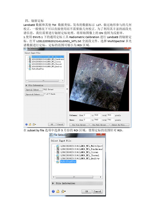
四，辐射定标Landsat8数据和其他TM 数据类似，发布的数据标示L1T，做过地形参与的几何校正，一般情况下可以直接使用而不需要做几何校正。

为了利用其丰富的波段光谱信息，我们需要进行辐射定标处理，将原始图像上的DN值转为反射率。

1.使用ENVI5.1下的通用定标工具Radiometric Calibration进行Landsat8的辐射定标。

打开LC81220382013141LGN01_MTL.txt全波段文件，选择MultiSpectral多光谱数据进行定标，定标的范围可缩小为ROI区域。

在subset by file选项中选择5月份的ROI区域，使得定标的范围针对ROI。

2.定标参数设置。

为后续的FLAASH大气校正做数据准备，单击Apply FLAASH Settings得到相应的参数。

辐射定标后的结果：通过定标之后的影像DN值可靠。

五．Flassh大气校正大气校正的意义在于去除一些大气的干扰，利用ENVI5.1工具箱中的FLAASH Atmospheric Correction进行大气校正。

大气校正参数设置：1) Input Radiance Image：打开辐射定标结果数据,要求为BIL存储格式；2) Output Reflectance File：设置输出FLAASH大气校正结果的路径；3) Output Directory for FLAASH Files：设置输出FLAASH校正文件的路径；4) Scene Center Location：自动获取；5) Sensor Type：Landsat-8 OLI；Sensor Altitude:自动读取；Pixel Size:自动读取；6) Ground Elevation: 0.132KM。

注：利用ENVI自带的全球900米分辨率DEM数据计算，Open World Data ->Elevation（GMTED2010）;在Toolbox下选择Statistics->Compute Statistics，打开Compute Statistics输入文件对话框，选择GMTED2010.jp2数据。

ASTM材料与实验标准.E94

Designation:E94–04Standard Guide forRadiographic Examination1This standard is issued under theﬁxed designation E94;the number immediately following the designation indicates the year of original adoption or,in the case of revision,the year of last revision.A number in parentheses indicates the year of last reapproval.A superscript epsilon(e)indicates an editorial change since the last revision or reapproval.1.Scope1.1This guide2covers satisfactory X-ray and gamma-ray radiographic examination as applied to industrial radiographic ﬁlm recording.It includes statements about preferred practice without discussing the technical background which justiﬁes the preference.A bibliography of several textbooks and standard documents of other societies is included for additional infor-mation on the subject.1.2This guide covers types of materials to be examined; radiographic examination techniques and production methods; radiographicﬁlm selection,processing,viewing,and storage; maintenance of inspection records;and a list of available reference radiograph documents.N OTE1—Further information is contained in Guide E999,Practice E1025,Test Methods E1030and E1032.1.3Interpretation and Acceptance Standards—Interpretation and acceptance standards are not covered by this guide,beyond listing the available reference radiograph docu-ments for castings and welds.Designation of accept-reject standards is recognized to be within the cognizance of product speciﬁcations and generally a matter of contractual agreement between producer and purchaser.1.4Safety Practices—Problems of personnel protection against X rays and gamma rays are not covered by this document.For information on this important aspect of radiog-raphy,reference should be made to the current document of the National Committee on Radiation Protection and Measure-ment,Federal Register,U.S.Energy Research and Develop-ment Administration,National Bureau of Standards,and to state and local regulations,if such exist.For speciﬁc radiation safety information refer to NIST Handbook ANSI43.3,21 CFR1020.40,and29CFR1910.1096or state regulations for agreement states.1.5This standard does not purport to address all of the safety problems,if any,associated with its use.It is the responsibility of the user of this standard to establish appro-priate safety and health practices and determine the applica-bility of regulatory limitations prior to use.(See1.4.)1.6If an NDT agency is used,the agency shall be qualiﬁed in accordance with Practice E543.2.Referenced Documents2.1ASTM Standards:3E543Practice for Evaluating Agencies that Perform Non-destructive TestingE746Test Method for Determining Relative Image Quality Response of Industrial Radiographic Film SystemsE747Practice for Design,Manufacture,and Material Grouping Classiﬁcation of Wire Image Quality Indicators (IQI)Used for RadiologyE801Practice for Controlling Quality of Radiological Ex-amination of Electronic DevicesE999Guide for Controlling the Quality of Industrial Ra-diographic Film ProcessingE1025Practice for Design,Manufacture,and Material Grouping Classiﬁcation of Hole-Type Image Quality Indi-cators(IQI)Used for RadiologyE1030Test Method for Radiographic Examination of Me-tallic CastingsE1032Test Method for Radiographic Examination of WeldmentsE1079Practice for Calibration of Transmission Densitom-etersE1254Guide for Storage of Radiographs and Unexposed Industrial Radiographic FilmsE1316Terminology for Nondestructive ExaminationsE1390Guide for Illuminators Used for Viewing Industrial RadiographsE1735Test Method for Determining Relative Image Qual-ity of Industrial Radiographic Film Exposed to X-Radiation from4to25MVE1742Practice for Radiographic ExaminationE1815Test Method for Classiﬁcation of Film Systems for Industrial Radiography2.2ANSI Standards:1This guide is under the jurisdiction of ASTM Committee E07on Nondestruc-tive Testing and is the direct responsibility of Subcommittee E07.01on Radiology (X and Gamma)Method.Current edition approved January1,2004.Published February2004.Originally approved st previous edition approved in2000as E94-00.2For ASME Boiler and Pressure Vessel Code applications see related Guide SE-94in Section V of that Code.3For referenced ASTM standards,visit the ASTM website,,or contact ASTM Customer Service at service@.For Annual Book of ASTM Standards volume information,refer to the standard’s Document Summary page on the ASTM website.Copyright©ASTM International,100Barr Harbor Drive,PO Box C700,West Conshohocken,PA19428-2959,United States.PH1.41Speciﬁcations for Photographic Film for Archival Records,Silver-Gelatin Type,on Polyester Base 4PH2.22Methods for Determining Safety Times of Photo-graphic Darkroom Illumination 4PH4.8Methylene Blue Method for Measuring Thiosulfate and Silver Densitometric Method for Measuring Residual Chemicals in Films,Plates,and Papers 4T9.1Imaging Media (Film)—Silver-Gelatin Type Speciﬁ-cations for Stability 4T9.2Imaging Media—Photographic Process Film Plate and Paper Filing Enclosures and Storage Containers 42.3Federal Standards:Title 21,Code of Federal Regulations (CFR)1020.40,Safety Requirements of Cabinet X-Ray Systems 5Title 29,Code of Federal Regulations (CFR)1910.96,Ionizing Radiation (X-Rays,RF,etc.)52.4Other Document:NBS Handbook ANSI N43.3General Radiation Safety Installations Using NonMedical X-Ray and Sealed Gamma Sources up to 10MeV 63.Terminology3.1Deﬁnitions —For deﬁnitions of terms used in this guide,refer to Terminology E 1316.4.Signiﬁcance and Use4.1Within the present state of the radiographic art,this guide is generally applicable to available materials,processes,and techniques where industrial radiographic ﬁlms are used as the recording media.4.2Limitations —This guide does not take into consider-ation special beneﬁts and limitations resulting from the use of nonﬁlm recording media or readouts such as paper,tapes,xeroradiography,ﬂuoroscopy,and electronic image intensiﬁ-cation devices.Although reference is made to documents that may be used in the identiﬁcation and grading,where appli-cable,of representative discontinuities in common metal cast-ings and welds,no attempt has been made to set standards of acceptance for any material or production process.Radiogra-phy will be consistent in sensitivity and resolution only if the effect of all details of techniques,such as geometry,ﬁlm,ﬁltration,viewing,etc.,is obtained and maintained.5.Quality of Radiographs5.1To obtain quality radiographs,it is necessary to consider as a minimum the following list of items.Detailed information on each item is further described in this guide.5.1.1Radiation source (X-ray or gamma),5.1.2V oltage selection (X-ray),5.1.3Source size (X-ray or gamma),5.1.4Ways and means to eliminate scattered radiation,5.1.5Film system class,5.1.6Source to ﬁlm distance,5.1.7Image quality indicators (IQI’s),5.1.8Screens and ﬁlters,5.1.9Geometry of part or component conﬁguration,5.1.10Identiﬁcation and location markers,and 5.1.11Radiographic quality level.6.Radiographic Quality Level6.1Information on the design and manufacture of image quality indicators (IQI’s)can be found in Practices E 747,E 801,E 1025,and E 1742.6.2The quality level usually required for radiography is 2%(2-2T when using hole type IQI)unless a higher or lower quality is agreed upon between the purchaser and the supplier.At the 2%subject contrast level,three quality levels of inspection,2-1T,2-2T,and 2-4T,are available through the design and application of the IQI (Practice E 1025,Table 1).Other levels of inspection are available in Practice E 1025Table 1.The level of inspection speciﬁed should be based on the service requirements of the product.Great care should be taken in specifying quality levels 2-1T,1-1T,and 1-2T by ﬁrst determining that these quality levels can be maintained in production radiography.N OTE 2—The ﬁrst number of the quality level designation refers to IQI thickness expressed as a percentage of specimen thickness;the second number refers to the diameter of the IQI hole that must be visible on the radiograph,expressed as a multiple of penetrameter thickness,T .6.3If IQI’s of material radiographically similar to that being examined are not available,IQI’s of the required dimensions but of a lower-absorption material may be used.6.4The quality level required using wire IQI’s shall be equivalent to the 2-2T level of Practice E 1025unless a higher or lower quality level is agreed upon between purchaser and supplier.Table 4of Practice E 747gives a list of various hole-type IQI’s and the diameter of the wires of corresponding EPS with the applicable 1T,2T,and 4T holes in the plaque IQI.Appendix X1of Practice E 747gives the equation for calcu-lating other equivalencies,if needed.7.Energy Selection7.1X-ray energy affects image quality.In general,the lower the energy of the source utilized the higher the achievable radiographic contrast,however,other variables such as geom-etry and scatter conditions may override the potential advan-tage of higher contrast.For a particular energy,a range of thicknesses which are a multiple of the half value layer,may be radiographed to an acceptable quality level utilizing a particu-lar X-ray machine or gamma ray source.In all cases the speciﬁed IQI (penetrameter)quality level must be shown on the radiograph.In general,satisfactory results can normally be obtained for X-ray energies between 100kV to 500kV in a range between 2.5to 10half value layers (HVL)of material thickness (see Table 1).This range may be extended by as much as a factor of 2in some situations for X-ray energies in the 1to 25MV range primarily because of reduced scatter.4Available from American National Standards Institute (ANSI),25W.43rd St.,4th Floor,New York,NY 10036.5Available from ernment Printing Office Superintendent of Documents,732N.Capitol St.,NW,Mail Stop:SDE,Washington,DC 20401.6Available from National Technical Information Service (NTIS),U.S.Depart-ment of Commerce,5285Port Royal Rd.,Springﬁeld,V A22161.8.Radiographic Equivalence Factors8.1The radiographic equivalence factor of a material is that factor by which the thickness of the material must be multi-plied to give the thickness of a “standard”material (often steel)which has the same absorption.Radiographic equivalence factors of several of the more common metals are given in Table 2,with steel arbitrarily assigned a factor of 1.0.The factors may be used:8.1.1To determine the practical thickness limits for radia-tion sources for materials other than steel,and8.1.2To determine exposure factors for one metal from exposure techniques for other metals.9.Film9.1Various industrial radiographic ﬁlm are available to meet the needs of production radiographic work.However,deﬁnite rules on the selection of ﬁlm are difficult to formulate because the choice depends on individual user requirements.Some user requirements are as follows:radiographic quality levels,exposure times,and various cost factors.Several methods are available for assessing image quality levels (see Test Method E 746,and Practices E 747and E 801).Informa-tion about speciﬁc products can be obtained from the manu-facturers.9.2Various industrial radiographic ﬁlms are manufactured to meet quality level and production needs.Test Method E 1815provides a method for ﬁlm manufacturer classiﬁcation of ﬁlm systems.A ﬁlm system consist of the ﬁlm andassociated ﬁlm processing ers may obtain a classi-ﬁcation table from the ﬁlm manufacturer for the ﬁlm system used in production radiography.A choice of ﬁlm class can be made as provided in Test Method E 1815.Additional speciﬁc details regarding classiﬁcation of ﬁlm systems is provided in Test Method E 1815.ANSI Standards PH1.41,PH4.8,T9.1,and T9.2provide speciﬁc details and requirements for ﬁlm manufacturing.10.Filters10.1Deﬁnition —Filters are uniform layers of material placed between the radiation source and the ﬁlm.10.2Purpose —The purpose of ﬁlters is to absorb the softer components of the primary radiation,thus resulting in one or several of the following practical advantages:10.2.1Decreasing scattered radiation,thus increasing con-trast.10.2.2Decreasing undercutting,thus increasing contrast.10.2.3Decreasing contrast of parts of varying thickness.10.3Location —Usually the ﬁlter will be placed in one of the following two locations:10.3.1As close as possible to the radiation source,which minimizes the size of the ﬁlter and also the contribution of the ﬁlter itself to scattered radiation to the ﬁlm.10.3.2Between the specimen and the ﬁlm in order to absorb preferentially the scattered radiation from the specimen.It should be noted that lead foil and other metallic screens (see 13.1)fulﬁll this function.10.4Thickness and Filter Material —The thickness and material of the ﬁlter will vary depending upon the following:10.4.1The material radiographed.10.4.2Thickness of the material radiographed.10.4.3Variation of thickness of the material radiographed.10.4.4Energy spectrum of the radiation used.10.4.5The improvement desired (increasing or decreasing contrast).Filter thickness and material can be calculated or determined empirically.11.Masking11.1Masking or blocking (surrounding specimens or cov-ering thin sections with an absorptive material)is helpful in reducing scattered radiation.Such a material can also be usedTABLE 1Typical Steel HVL Thickness in Inches [mm]forCommon EnergiesEnergyThickness,Inches [mm]120kV 0.10[2.5]150kV 0.14[3.6]200kV 0.20[5.1]250kV0.25[6.4]400kV (Ir 192)0.35[8.9]1MV0.57[14.5]2MV (Co 60)0.80[20.3]4MV 1.00[25.4]6MV 1.15[29.2]10MV1.25[31.8]16MV and higher1.30[33.0]TABLE 2Approximate Radiographic Equivalence Factors for Several Metals (Relative to Steel)MetalEnergy Level100kV 150kV 220kV 250kV400kV1MV2MV4to 25MV192Ir60CoMagnesium 0.050.050.08Aluminum0.080.120.180.350.35Aluminum alloy 0.100.140.180.350.35Titanium0.540.540.710.90.90.90.90.9Iron/all steels 1.0 1.0 1.0 1.0 1.0 1.0 1.0 1.0 1.0 1.0Copper 1.51.6 1.4 1.41.4 1.1 1.1 1.2 1.1 1.1Zinc 1.4 1.3 1.3 1.2 1.1 1.0Brass 1.4 1.3 1.3 1.2 1.1 1.0 1.1 1.0Inconel X 1.4 1.3 1.3 1.3 1.3 1.3 1.3 1.3Monel 1.7 1.2Zirconium2.4 2.3 2.0 1.7 1.5 1.0 1.0 1.0 1.2 1.0Lead 14.014.012.0 5.0 2.52.7 4.0 2.3Hafnium 14.012.09.03.0Uranium20.016.012.04.03.912.63.4to equalize the absorption of different sections,but the loss of detail may be high in the thinner sections.12.Back-Scatter Protection12.1Effects of back-scattered radiation can be reduced by conﬁning the radiation beam to the smallest practical cross section and by placing lead behind theﬁlm.In some cases either or both the back lead screen and the lead contained in the back of the cassette orﬁlm holder will furnish adequate protection against back-scattered radiation.In other instances, this must be supplemented by additional lead shielding behind the cassette orﬁlm holder.12.2If there is any question about the adequacy of protec-tion from back-scattered radiation,a characteristic symbol (frequently a1⁄8-in.[3.2-mm]thick letter B)should be attached to the back of the cassette orﬁlm holder,and a radiograph made in the normal manner.If the image of this symbol appears on the radiograph as a lighter density than background, it is an indication that protection against back-scattered radia-tion is insufficient and that additional precautions must be taken.13.Screens13.1Metallic Foil Screens:13.1.1Lead foil screens are commonly used in direct contact with theﬁlms,and,depending upon their thickness, and composition of the specimen material,will exhibit an intensifying action at as low as90kV.In addition,any screen used in front of theﬁlm acts as aﬁlter(Section10)to preferentially absorb scattered radiation arising from the speci-men,thus improving radiographic quality.The selection of lead screen thickness,or for that matter,any metallic screen thickness,is subject to the same considerations as outlined in 10.4.Lead screens lessen the scatter reaching theﬁlm regard-less of whether the screens permit a decrease or necessitate an increase in the radiographic exposure.To avoid image unsharp-ness due to screens,there should be intimate contact between the lead screen and theﬁlm during exposure.13.1.2Lead foil screens of appropriate thickness should be used whenever they improve radiographic quality or penetram-eter sensitivity or both.The thickness of the front lead screens should be selected with care to avoid excessiveﬁltration in the radiography of thin or light alloy materials,particularly at the lower kilovoltages.In general,there is no exposure advantage to the use of0.005in.in front and back lead screens below125 kV in the radiography of1⁄4-in.[6.35-mm]or lesser thickness steel.As the kilovoltage is increased to penetrate thicker sections of steel,however,there is a signiﬁcant exposure advantage.In addition to intensifying action,the back lead screens are used as protection against back-scattered radiation (see Section12)and their thickness is only important for this function.As exposure energy is increased to penetrate greater thicknesses of a given subject material,it is customary to increase lead screen thickness.For radiography using radioac-tive sources,the minimum thickness of the front lead screen should be0.005in.[0.13mm]for iridium-192,and0.010in.[0.25mm]for cobalt-60.13.2Other Metallic Screen Materials:13.2.1Lead oxide screens perform in a similar manner to lead foil screens except that their equivalence in lead foil thickness approximates0.0005in.[0.013mm].13.2.2Copper screens have somewhat less absorption and intensiﬁcation than lead screens,but may provide somewhat better radiographic sensitivity with higher energy above1MV.13.2.3Gold,tantalum,or other heavy metal screens may be used in cases where lead cannot be used.13.3Fluorescent Screens—Fluorescent screens may be used as required providing the required image quality is achieved.Proper selection of theﬂuorescent screen is required to minimize image unsharpness.Technical information about speciﬁcﬂuorescent screen products can be obtained from the manufacturers.Goodﬁlm-screen contact and screen cleanli-ness are required for successful use ofﬂuorescent screens. Additional information on the use ofﬂuorescent screens is provided in Appendix X1.13.4Screen Care—All screens should be handled carefully to avoid dents and scratches,dirt,or grease on active surfaces. Grease and lint may be removed from lead screens with a solvent.Fluorescent screens should be cleaned in accordance with the recommendations of the manufacturer.Screens show-ing evidence of physical damage should be discarded.14.Radiographic Image Quality14.1Radiographic image quality is a qualitative term used to describe the capability of a radiograph to showﬂaws in the area under examination.There are three fundamental compo-nents of radiographic image quality as shown in Fig.1.Each component is an important attribute when considering a speciﬁc radiographic technique or application and will be brieﬂy discussed below.14.2Radiographic contrast between two areas of a radio-graph is the difference between theﬁlm densities of those areas.The degree of radiographic contrast is dependent upon both subject contrast andﬁlm contrast as illustrated in Fig.1.14.2.1Subject contrast is the ratio of X-ray or gamma-ray intensities transmitted by two selected portions of a specimen. Subject contrast is dependent upon the nature of the specimen (material type and thickness),the energy(spectral composition, hardness or wavelengths)of the radiation used and the intensity and distribution of scattered radiation.It is independent of time,milliamperage or source strength(curies),source distance and the characteristics of theﬁlm system.14.2.2Film contrast refers to the slope(steepness)of the ﬁlm system characteristic curve.Film contrast is dependent upon the type ofﬁlm,the processing it receives and the amount ofﬁlm density.It also depends upon whether theﬁlm was exposed with lead screens(or without)or withﬂuorescent screens.Film contrast is independent,for most practical purposes,of the wavelength and distribution of the radiation reaching theﬁlm and,hence is independent of subject contrast. For further information,consult Test Method E1815.14.3Film system granularity is the objective measurement of the local density variations that produce the sensation of graininess on the radiographicﬁlm(for example,measured with a densitometer with a small aperture of#0.0039in.[0.1 mm]).Graininess is the subjective perception of a mottled random pattern apparent to a viewer who sees smalllocaldensity variations in an area of overall uniform density (that is,the visual impression of irregularity of silver deposit in a processed radiograph).The degree of granularity will not affect the overall spatial radiographic resolution (expressed in line pairs per mm,etc.)of the resultant image and is usually independent of exposure geometry arrangements.Granularity is affected by the applied screens,screen-ﬁlm contact and ﬁlm processing conditions.For further information on detailed perceptibility,consult Test Method E 1815.14.4Radiographic deﬁnition refers to the sharpness of the image (both the image outline as well as image detail).Radiographic deﬁnition is dependent upon the inherent un-sharpness of the ﬁlm system and the geometry of the radio-graphic exposure arrangement (geometric unsharpness)as illustrated in Fig.1.14.4.1Inherent unsharpness (U i )is the degree of visible detail resulting from geometrical aspects within the ﬁlm-screen system,that is,screen-ﬁlm contact,screen thickness,total thickness of the ﬁlm emulsions,whether single or double-coated emulsions,quality of radiation used (wavelengths,etc.)and the type of screen.Inherent unsharpness is independent of exposure geometry arrangements.14.4.2Geometric unsharpness (U g )determines the degree of visible detail resultant from an “in-focus”exposure arrange-ment consisting of the source-to-ﬁlm-distance,object-to-ﬁlm-distance and focal spot size.Fig.2(a)illustrates these condi-tions.Geometric unsharpness is given by the equation:U g 5Ft /d o(1)where:U g =geometric unsharpness,F =maximum projected dimension of radiation source,t =distance from source side of specimen to ﬁlm,and d o =source-object distance.N OTE 3—d o and t must be in the same units of measure;the units of U g will be in the same units as F .N OTE 4—A nomogram for the determination of U g is given in Fig.3(inch-pound units).Fig.4represents a nomogram in metric units.Example:Given:Source-object distance (d o )=40in.,Source size (F)=500mils,andSource side of specimen to ﬁlm distance (t)=1.5in.Draw a straight line (dashed in Fig.3)between 500mils on the F scale and 1.5in.on the t scale.Note the point on intersection (P)of this line with the pivot line.Draw a straight line (solid in Fig.3)from 40in.on the d o scale through point P and extend to the U g scale.Intersection of this line with the U g scale gives geometrical unsharpness in mils,which in the example is 19mils.Inasmuch as the source size,F ,is usually ﬁxed for a given radiation source,the value of U g is essentially controlled by the simple d o /t ratio.Geometric unsharpness (U g )can have a signiﬁcant effect on the quality of the radiograph;therefore source-to-ﬁlm-distance (SFD)selection is important.The geometric unsharpness (U g )equation,Eq 1,is for information and guidance and provides a means for determining geometric unsharpness values.The amount or degree of unsharpness should be minimized when establishing the radiographic technique.Radiographic Image QualityRadiographic ContrastFilm System Granularity Radiographic DeﬁnitionSubject Contrast Film Contrast •Grain size and distribution within the ﬁlm emulsion •Processing conditions(type and activity of developer,temperature of developer,etc.)•Type ofscreens (that is,ﬂuorescent,lead or none)•Radiation quality (that is,energy level,ﬁltration,etc.•Exposure quanta (that is,intensity,dose,etc.)InherentUnsharpness Geometric Unsharpness Affected by:•Absorption differences in specimen (thickness,composition,density)•Radiation wavelength •Scattered radiationAffected by:•Type of ﬁlm•Degree of development (type of developer,time,temperature and activity of developer,degree of agitation)•Film density •Type ofscreens (that is,ﬂuorescent,lead or none)Affected by:•Degree of screen-ﬁlm contact •Total ﬁlm thickness •Single ordouble emulsion coatings •Radiation quality •Type and thickness of screens (ﬂuorescent,lead or none)Affected by:•Focal spot or source physical size •Source-to-ﬁlm distance •Specimen-to-ﬁlm distance•Abruptness of thickness changes in specimen •Motion of specimen or radiation sourceReduced or enhanced by:•Masks and diaphragms •Filters•Lead screens •Potter-Bucky diaphragmsFIG.1Variables of Radiographic ImageQualityFIG.2Effects of Object-Film Geometry15.Radiographic Distortion15.1The radiographic image of an object or feature within an object may be larger or smaller than the object or feature itself,because the penumbra of the shadow is rarely visible in a radiograph.Therefore,the image will be larger if the object or feature is larger than the source of radiation,and smaller if object or feature is smaller than the source.The degree of reduction or enlargement will depend on the source-to-object and object-to-ﬁlm distances,and on the relative sizes of the source and the object or feature (Fig.2(b )and (c )).15.2The direction of the central beam of radiation should be perpendicular to the surface of the ﬁlm whenever possible.The object image will be distorted if the ﬁlm is not aligned perpendicular to the central beam.Different parts of the object image will be distorted different amount depending on the extent of the ﬁlm to central beam offset (Fig.2(d )).16.Exposure Calculations or Charts16.1Development or procurement of an exposure chart or calculator is the responsibility of the individual laboratory.16.2The essential elements of an exposure chart or calcu-lator must relate the following:16.2.1Source or machine,16.2.2Material type,16.2.3Material thickness,16.2.4Film type (relative speed),16.2.5Film density,(see Note 5),16.2.6Source or source to ﬁlm distance,16.2.7Kilovoltage or isotope type,N OTE 5—For detailed information on ﬁlm density and density measure-ment calibration,see Practice E 1079.16.2.8Screen type andthickness,FIG.3Nomogram for Determining Geometrical Unsharpness (Inch-PoundUnits)16.2.9Curies or milliampere/minutes,16.2.10Time of exposure,16.2.11Filter (in the primary beam),16.2.12Time-temperature development for hand process-ing;access time for automatic processing;time-temperature development for dry processing,and16.2.13Processing chemistry brand name,if applicable.16.3The essential elements listed in 16.2will be accurate for isotopes of the same type,but will vary with X-ray equipment of the same kilovoltage and milliampere rating.16.4Exposure charts should be developed for each X-ray machine and corrected each time a major component is replaced,such as the X-ray tube or high-voltage transformer.16.5The exposure chart should be corrected when the processing chemicals are changed to a different manufacturer’s brand or the time-temperature relationship of the processormay be adjusted to suit the exposure chart.The exposure chart,when using a dry processing method,should be corrected based upon the time-temperature changes of the processor.17.Technique File17.1It is recommended that a radiographic technique log or record containing the essential elements be maintained.17.2The radiographic technique log or record should con-tain the following:17.2.1Description,photo,or sketch of the test object illustrating marker layout,source placement,and ﬁlm location.17.2.2Material type and thickness,17.2.3Source to ﬁlm distance,17.2.4Film type,17.2.5Film density,(see Note 5),17.2.6Screen type andthickness,FIG.4Nomogram for Determining Geometrical Unsharpness (MetricUnits)。

Johnson 准则

Results from a Range of Blackbodies: Difference Between Measured and Predicted Radiance Temperatures
Intl. Workshop on Radiometric & Geometric Calibration Dec 2003
Page 1
C. Johnson
NIST Overview
• The U.S. metrology and standards laboratory • Non-regulatory agency in Dept. of Commerce • Promotes U.S. economic growth by working with industry to develop and apply technology, measurements, & standards • Four main components: – Measurement and Standards Laboratories – Advanced Technology Program – Manufacturing Extension Partnership – National Quality Program
Page 9 C. Johnson
Intl. Workshop on Radiometric & Geometric Calibration Dec 2003
SIRCUS Experimental Layout
Tunable Laser
Intensity Stabilizer Chopper or Shutter Wavemeter
CO

CIE 标准美国照明协会标准大全

CIE 标准美国照明协会标准大全CIE 1-1980 Guide Lines for Minimizing Urban Sky Glow Near Astronomical Observatories (E)CIE 13.3-1995 Method of Measuring and Specifying Colour Rendering Properties of Light Sources (E)CIE 15-2004 Colorimetry - Third Edition;CIE 16-1970 Daylight (1st Edition) (E)CIE 17.4-1987 International Lighting Vocabulary (E) (F) (G) (R)CIE 18.2-1983 Basis of Physical Photometry (E)CIE 19/2.1-1981 An Analytic Model for Describing the Influence of Lighting Parameters Upon Visual Performance: Volume 1: Technical Foundations (E)CIE 19/2.2-1981 An Analytic Model for Describing the Influence of Lighting Parameters Upon Visual Performance: Volume II: Summary and Application Guidelines (E)CIE 23-1973 International Recommendations for Motorway Lighting (CIE 23.1-1996 Revision 1) (E)CIE 31-1976 Glare and Uniformity in Road Lighting Installations (E)CIE 32-1977 Lighting in Situations Requiring Special Treatment (CIE 32.1-1996 Revision 1) (E) (F)CIE 33-1977 Depreciation of Installations and Their Maintenance (CIE 33.1-1996 Revision 1) (E) (F)CIE 34-1977 Road Lighting Lantern and Installation Data - Photometrics, Classification and Performance (E)CIE 38-1977 Radiometric and Photometric Characteristics of Materials and Their Measurement (E) (F) (G)CIE 39.2-1983 Recommendations for Surface Colours for Visual Signalling (CIE 39.3-1996 Revision 1) (E)CIE 40-1978 Calculations for Interior Lighting: Basic Method - CIE 40.1-1996; Revision 1; (E)CIE 41-1978 Light as a True Visual Quantity: Principles of Measurement (1st Edition) (Reprint 1994) (E)CIE 42-1978 Lighting for Tennis (E)CIE 43-1979 Photometry of Floodlights (E)CIE 44-1979 Absolute Methods for Reflection Measurement (1st Edition) (Reprint 1990) (E)CIE 45-1979 Lighting for Ice Sports (E)CIE 46-1979 A Review of Publications on Properties and Reflection Values of Material Reflection Standards (E)CIE 47-1979 Road Lighting for Wet Conditions (E)CIE 48-1980 Light Signals for Road Traffic Control (E)CIE 49-1981 Guide on the Emergency Lighting of Building Interiors (E)CIE 51.2-1999 A METHOD FOR ASSESSING THE QUALITY OF DAYLIGHT SIMULATORS FOR COLORIMETRY - Incorporating supplement 1CIE 52-1982 Calculations for Interior Lighting Applied Method (E)CIE 53-1982 Methods of Characterizing the Performance of Radiometers and Photometers (E)CIE 54.2-2001 RETROREFLECTION: DEFINITION AND MEASUREMENTCIE 55-1983 Discomfort Glare in the Interior Working Environment (E)CIE 57-1983 Lighting for Football (E)CIE 58-1983 Lighting for Sports Halls (E)CIE 59-1984 Polarization: Definitions and Nomenclature, Instrument Polarization (E)CIE 60-1984 Vision and the Visual Display Unit Work Station (E)CIE 61-1984 Tunnel Entrance Lighting: A Survey of Fundamentals for Determining the Luminance in the Threshold Zone (E)CIE 62-1984 Lighting for Swimming Pools (E)CIE 63-1984 The Spectroradiometric Measurement of Light Sources (E)CIE 64-1984 Determination of the Spectral Responsivity of Optical Radiation Detectors (E)CIE 65-1985 Electrically Calibrated Thermal Detectors of Optical Radiation: (Absolute Radiometers) (E)CIE 66-1984 Road Surfaces and Lighting: Joint Technical Report CIE/PIARC (E)CIE 67-1986 Guide for the Photometric Specification and Measurement of Sports Lighting Installations (E)CIE 69-1987 Methods of Characterizing Illuminance Meters and Luminance Meters: Performance, Characteristics and Specifications (E) CIE 70-1987 Measurement of Absolute Luminous Intensity Distributions (E)CIE 72-1987 Guide to the Properties and Uses of Retroreflectors at Night (E)CIE 73-1988 Visual Aspects of Road Markings: Joint Technical Report CIE/PIARC (E)CIE 74-1988 Roadsigns (E)CIE 75-1988 Spectral Luminous Efficiency Functions Based Upon Brightness Matching for Monochromatic Point Sources 2 Degree and 10 Degree Fields (E)CIE 76-1988 Intercomparison on Measurement of (Total) Spectral Radiance Factor of Luminescent Specimens (1st Edition) (Reprint 1990) (E) CIE 77-1988 Electric Light Sources State of the Art - 1987 (E)CIE 78-1988 Brightness Luminance Relations: Classified Bibliography (E)CIE 79-1988 A Guide for the Design of Road Traffic Lights (1st Edition) (Reprint 1992) (E)CIE 80-1989 Special Metamerism Index: Change in Observer (1st Edition) (E)CIE 81-1989 Mesopic Photometry: History, Special Problems and Practical Solutions (1st Edition) (E)CIE 82-1990 History of the CIE: 1913-1918 (E)CIE 83-1989 Guide for the Lighting of Sports Events for Colour Television and Film Systems (2nd Edition) (E)CIE 84-1989 Measurement of Luminous Flux (1st Edition) (E)CIE 85-1989 Solar Spectral Irradiance (1st Edition) (E)CIE 86-1990 CIE 1988 2 Degree Spectral Luminous Efficiency Function for Photopic Vision (1st Edition) (E)CIE 87-1990 Colorimetry of Self-Luminous Displays - A Bibliography (1st Edition) (E)CIE 88-2004 Guide for the Lighting of Road Tunnels and Underpasses - 2nd Edition (D)CIE 89-1991 Technical Collection 1990 (E)CIE 90-1991 Sunscreen Testing (UV.B) (1st Edition) (E)CIE 93-1992 Road Lighting as an Accident Countermeasure (1st Edition) (E)CIE 94-1993 Guide for Floodlighting (1st Edition) (E)CIE 95-1992 Contrast and Visibility (1st Edition) (E)CIE 96-1992 Electric Light Sources State of the Art - 1991 (1st Edition) (E)CIE 97-2005 Guide on the Maintenance of Indoor Electric Lighting Systems - Second EditionCIE 98-1992 Personal Dosimetry of UV Radiation (1st Edition) (E)CIE 99-1992 Lighting Education (1983 - 1989) (1st Edition) (E)CIE 100-1992 Fundamentals of the Visual Task of Night Driving (1st Edition) (E)CIE 101-1993 Parametric Effects in Colour-Difference Evaluation (1st Edition) (E)CIE 102-1993 Recommended File Format for Electronic Transfer of Luminaire Photometric Data (1st Edition) (E)CIE 103-1993 Technical Collection 1993 (1st Edition) (E)CIE 104-1993 Daytime Running Lights (DRL) (1st Edition) (E)CIE 105-1993 Spectroradiometry of Pulsed Optical Radiation Sources (1st Edition) (E)CIE 106-1993 CIE Collection in Photobiology and Photochemistry (1st Edition) (E)CIE 107-1994 Review of the Offical Recommendations of the CIE for the Colours of Signal Lights (E)CIE 108-1994 Guide to Recommended Practice of Daylight Measurement (E)CIE 109-1994 A Method of Predicting Corresponding Colours Under Different Chromatic and Illuminance Adaptations (CIE 109CIE 110-1994 Spatial Distribution of Daylight - Luminance Distributions of Various Reference Skies (CIE 110.1-1995 Revision 1)CIE 111-1994 Variable Message Signs (E)CIE 112-1994 Glare Evaluation System for Use Within Outdoor Sports and Area Lighting (E)CIE 113-1995 Maintained Night-Time Visibility of Retroreflective Road Signs (E)CIE 114-1994 CIE Collection in Photometry and Rodiometry (E)CIE 115-1995 Recommendations for the Lighting of Roads for Motor and Pedestrian Traffic (E)CIE 116-1995 Industrial Colour-Difference Evaluation (E)CIE 117-1995 Technical Report Discomfort Glare in Interior LightingCIE 118-1995 CIE Collection in Colour and VisionCIE 119-1995 23RD Session of the CIE New Delhi November 1-8, 1995 Volume 1 - Table of Contents OnlyCIE 121-SP1-2009 THE PHOTOMETRY AND GONIOPHOTOMETRY OF LUMINAIRES 鈥?SUPPLEMENT 1: LUMINAIRES FOR EMERGENCY LIGHTINGCIE 121-1996 The Photometry and Goniophotometry of LuminairesCIE 122-1996 Technical Report the Relationship Between Digital and Colorimetric Data for Computer-Controlled CRT DisplaysCIE 123-1997 Low Vision Lighting Needs for the Partially SightedCIE 124-1997 CIE Collection in Colour and Vision 1997CIE 125-1997 Standard Erythema Dose a ReviewCIE 126-1997 Guidelines for Minimizing Sky GlowCIE 127-2007 Measurement of LEDs - Second EditionCIE 128-1998 Guide to the Lighting for Open-Cast MinesCIE 129-1998 Guide for Lighting Exterior Work AreasCIE 130-1998 Practical Methods for the Measurement of Reflectance and TransmittanceCIE 132-1999 Design Methods for Lighting of RoadsCIE 133 VOL-1999 24th Session of the CIE Warsaw - June 24-30, 1999CIE 133 VOL-1999 24th Session of the CIE Warsaw - June 24-30, 1999CIE 134-1999 CIE Collection in Photobiology and Photochemistry 1999CIE 135-1999 CIE Collection 1999; Vision and Colour; Physical Measurement of Light and Radiation - Revision 1 - February 2000CIE 136-2000 Technical Report; Guide to the Lighting of Urban AreasCIE 137-2000 Technical Report; Conspicuity of Traffic Signs in Complex BackgroundsCIE 138-2000 CIE Collection in Photobiology and Photochemistry 2000CIE 139-2001 Influence of Daylight and Artificial Light on Diural and Seasonal Variations in Humans. A BibliographyCIE 140-2000 Road Lighting Calculations - Revision 2: December 2006CIE 141-2001 Testing of Supplementary Systems of PhotometryCIE 142-2001 Improvement to Industrial Colour-Difference EvaluationCIE 143-2001 International Recommendations for Colour Vision Requirements for TransportCIE 144-2001 ROAD SURFACE AND ROAD MARKING REFLECTION CHARACTERISTICSCIE 145-2002 THE CORRELATION OF MODELS FOR VISION AND VISUAL PERFORMANCECIE 146/147-2002 CIE COLLECTION on GLARE 2002CIE 148-2002 ACTION SPECTROSCOPY OF SKIN WITH TUNABLE LASERSCIE 149-2002 THE USE OF TUNGSTEN FILAMENT LAMPS AS SECONDARY STANDARD SOURCESCIE 150-2003 GUIDE ON THE LIMITATION OF THE EFFECTS OF OBTRUSIVE LIGHT FROM OUTDOOR LIGHTING INSTALLATIONSCIE 151-2003 SPECTRAL WEIGHTING OF SOLAR ULTRA VIOLET RADIATIONCIE 153-2003 REPORT ON AN INTERCOMPARISON OF MEASUREMENTS OF THE LUMINOUS FLUX OF HIGHPRESSURE SODIUM LAMPS - (A)CIE 154-2003 THE MAINTENANCE OF OUTDOOR LIGHTING SYSTEMS - (C)CIE 155-2003 ULTRA VIOLET AIR DISINFECTION - (G)CIE 156-2004 GUIDELINES FOR THE EV ALUATION OF GAMUT MAPPING ALGORITHMS - (C)CIE 157-2004 CONTROL OF DAMAGE TO MUSEUM OBJECTS BY OPTICAL RADIATION - (D)CIE 158-2004 OCULAR LIGHTING EFFECTS ON HUMAN PHYSIOLOGY AND BEHA VIOUR - (F)CIE 159-2004 A COLOUR APPEARANCE MODEL FOR COLOUR MANAGEMENT SYSTEMS: CIECAM02 - (C)CIE 160-2004 A REVIEW OF CHROMATIC ADAPTATION TRANSFORMS - (D)CIE 161-2004 LIGHTING DESIGN METHODS FOR OBSTRUCTED INTERIORSCIE 162-2004 CHROMATIC ADAPTATION UNDER MIXED ILLUMINATION CONDITION WHEN COMPARING SOFTCOPY AND HARDCOPY IMAGES - (C)CIE 163-2004 THE EFFECTS OF FLUORESCENCE IN THE CHARACTERIZATION OF IMAGING MEDIA - (B)CIE 164-2005 HOLLOW LIGHT GUIDE TECHNOLOGY AND APPLICATIONSCIE 165-2005 CIE 10 DEGREE PHOTOPIC PHOTOMETRIC OBSERVERCIE 167-2005 RECOMMENDED PRACTICE FOR TABULATING SPECTRAL DATA FOR USE IN COLOUR COMPUTATIONSCIE 168-2005 CRITERIA FOR THE EV ALUATION OF EXTENDED-GAMUT COLOUR ENCODINGSCIE 169-2005 PRACTICAL DESIGN GUIDELINES FOR THE LIGHTING OF SPORT EVENTS FOR COLOUR TELEVISION AND FILMING CIE 170-1-2006 FUNDAMENTAL CHROMATICITY DIAGRAM WITH PHYSIOLOGICAL AXES 鈥?PART 1CIE 171-2006 TEST CASES TO ASSESS THE ACCURACY OF LIGHTING COMPUTER PROGRAMSCIE 172-2006 UV PROTECTION AND CLOTHINGCIE 173-2006 TUBULAR DAYLIGHT GUIDANCE SYSTEMSCIE 174-2006 ACTION SPECTRUM FOR THE PRODUCTION OF PREVITAMIN D3 IN HUMAN SKINCIE 175-2006 A FRAMEWORK FOR THE MEASUREMENT OF VISUAL APPEARANCE - BilingualCIE 176-2006 GEOMETRIC TOLERANCES FOR COLOUR MEASUREMENTS - BilingualCIE 177-2007 COLOUR RENDERING OF WHITE LED LIGHT SOURCESCIE 178 VOL 1-1-2007 26TH SESSION OF THE CIE BEIJING - 4 JULY - 11 JULY 2007 PROCEEDINGS Volume 1 Part 1CIE 178 VOL 1-2-2007 26TH SESSION OF THE CIE BEIJING - 4 JULY - 11 JULY 2007 PROCEEDINGS Volume 1 Part 2CIE 178 VOL 2-2007 26TH SESSION OF THE CIE BEIJING - 4 JULY - 11 JULY 2007 PROCEEDINGS Volume 2CIE 179-2007 METHODS FOR CHARACTERISING TRISTIMULUS COLORIMETERS FOR MEASURING THE COLOUR OF LIGHT CIE 180-2007 ROAD TRANSPORT LIGHTING FOR DEVELOPING COUNTRIESCIE 181-2007 HAND PROTECTION BY DISPOSABLE GLOVES AGAINST OCCUPATIONAL UV EXPOSURECIE 182-2007 CALIBRATION METHODS AND PHOTOLUMINESCENT STANDARDS FOR TOTAL RADIANCE FACTOR MEASUREMENTSCIE 183-2008 DEFINITION OF THE CUT-OFF OF VEHICLE HEADLIGHTSCIE 184-2009 INDOOR DAYLIGHT ILLUMINANTSCIE S 004/E-2001 Colours of Light SignalsCIE S 005/E-1998 CIE Standard Illuminants for Colorimetry - ISO 10526: 1999CIE S 006.1/E-1999 Road Traffic Lights - Photometric Properties of 200 mm Roundel Signals - First Edition; ISO 16508CIE S 007/E-1998 Erythema Reference Action Spectrum and Standard Erythema Dose - ISO 17166: 1999CIE S 008/E-2001 Lighting of Indoor Work PlacesCIE S 009/E-2006 Photobiological Safety of Lamps and Lamp SystemsCIE S 010/E-2004 Photometry The CIE system of physical photometry - (E)CIE S 010/E-2004 PHOTOMETRY - THE CIE SYSTEM OF PHYSICAL PHOTOMETRY - (E)CIE S 011/E-2003 Spatial Distribution of Daylight - CIE Standard General SkyCIE S 012/E-2004 Standard method of assessing the spectral quality of daylight simulators for visual appraisal and measurement of colour - (E) CIE S 013/E-2003 International Standard Global Solar UV IndexCIE S 014-1/E-2006 Colorimetry 鈥?Part 1: CIE standard colorimetric observersCIE S 014-2/E-2006 Colorimetry - Part 2: CIE Standard IlluminantsCIE S 014-4/E-2007 Colorimetry 鈥?Part 4: CIE 1976 L*a*b* Colour spaceCIE S 015/E-2005 Lighting of Outdoor Work PlacesCIE S 019/E-2006 Photocarcinogenesis Action Spectrum (Non-Melanoma Skin Cancers) - (E)CIE S 020/E-2007 Emergency LightingCIE X005-1992 Proceedings of the CIE Seminar on Computer Programs for Light and Lighting: 5-9 October 1992 CIE Central Bureau Vienna, Austria (Table of Contents Only) (E)CIE X006-1991 Japan CIE Session at Prakash 91: Papers Presented by Japanese CIE Members in New Delhi,India, from October 7th to 13th, 1991 (Table of Contents Only) (E)CIE X007-1993 Proceedings of the CIE Symposium on Advanced Colorimetry: 8-10 June 1993 CIE Central Bureau Vienna, Austria (Table of Contents Only) (E)CIE X008-1994 Urban Sky Glow, A Worry for Astronomy: Proceedings of a Symposium of CIE TC 4-21: 3 April 1993 Royal Observatory Edinburgh, Scotland (Table of Contents Only) (E)CIE X009-1995 Proceedings of the CIE Symposium on Advances in Photometry: 1-3 December 1994 CIE Central Bureau, Vienna, Austria (Table of Contents Only) (E)CIE X010-1996 Proceedings of the CIE Expert Symposium 麓96 Colour Standards for Image Technology 25 - 27 March 1996 at the CIE Central Bureau Vienna, Austria - Table of Contents OnlyCIE X011-1996 Special Volume 23rd Session of the CIE New Delhi, November 1-8, 1995 Late Papers - Table of Contents OnlyCIE X012-1997 Proceedings of the NPL - CIE-UK Conference Visual Scales; Photometric and Colorimetric Aspects; 24 - 26 March 1997 at the National Physical Laboratory Teddington, UKCIE X013-1997 Proceedings of the CIE LED Symposium 麓97 on Standard Methods for Specifying and Measuring LED Characteristics; 24 - 25 October 1997 at the CIE Central Bureau Vienna, AustriaCIE X014-1998 Proceedings of the CIE Expert Symposium 麓97 on Colour Standards for Imaging Technology 21-22 November 1997 at the Radisson Resort Scottsdale, Arizona USACIE X015-1998 Proceedings of the First CIE Cymposium on Lighting Quality 9 - 10 May 1998 at the National Research Council Canada Ottowa, Ontario CanadaCIE X016-1998 Reference Book Based on Presentation Given by Health and Safety Experts on Optical Radiation Hazards; September 1-3, 1998; Gaithersburg, Maryland, USA (Table of Contents Only) (E)CIE X017-2000 Special Volume; 24th Session of the CIE; Warsaw, June 24 - 30, 1999; Late Papers (Table of Content Only) (E)CIE X018-1999 Proceedings of the CIE Symposium '99; 75 Years of CIE Photometry; 30 September - 02 October 1999 at the Hungarian Academy of Sciences; Budapest, Hungary (Table of Contents Only) (E)CIE X019-2001 Proceedings of Three CIE Workshops on Criteria for Road Lighting - Durban, Sourth Africa, 1997; Bath, United Kindgom, 1998; Warsaw, Poland, 1999CIE X020-2001 Proceedings of the CIE Expert Symposium 2001 on Uncertainty Evaluation Methods for Analysis of Uncertainties in Optical Radiation Measurement - 23 - 24 January 2001 at the CIE Cental Bureau; Vienna, AustriaCIE X021-2001 PROCEEDINGS of the CIE Expert Symposium 2000 on Extended Range Colour SpacesCIE X022-2001 PROCEEDINGS of the 2nd CIE Expert Symposium on LED Measurement Standard methods for specifying and measuring LED and LED cluster characteristicsCIE X023-2002 Proceedings of two CIE Worshops on Photometric Measurement Systems for Road Lighting InstallationsCIE X024-2002 PROCEEDINGS of the CIE/ARUP Symposium on Visual EnvironmentCIE X025-2002 PROCEEDINGS of the CIE Symposium '02 Temporal and Spatial Aspects of Light and Colour Perception and MeasurementCIE X026-2004 PROCEEDINGS of the CIE Symposium '04 LED Light Sources: Physical Measurement and Visual and Photobiological Assessment - Second Edition; CD-ROM INCLUDEDCIE X027-2004 PROCEEDINGS of the CIE Symposium '04 Light and Health: non-visual effects - CD-ROM INCLUDEDCIE X028-2005 PROCEEDINGS of the CIE Symposium '05 Vision and Lighting in Mesopic Conditions - CD-ROM INCLUDEDCIE X029-2006 PROCEEDINGS of the 2nd CIE Expert Symposium on Measurement UncertaintyCIE X030-2006 PROCEEDINGS of the ISCC/CIE Expert Symposium '06 75 Years of the CIE Standard Colorimetric Observer - 16 - 17 May 2006 National Research Council of Canada Ottawa, Ontario, Canada; Includes CD-ROMCIE X031-2006 PROCEEDINGS of the 2nd CIE Expert Symposium on Lighting and Health - CD-ROM INCLUDEDCIE X032-2007 Proceedings of the CIE Expert Symposium VISUAL APPEARANCE 19-20 October 2006, Paris, FranceCIE X033-2008 PROCEEDINGS of the CIE Expert Symposium on Advances in Photometry and Colorimetry 7-8 July 2008 Hotel Concorde Turin, Italy - CD-ROM INCLUDED。

辐射照度和光照度转换公式(一)

辐射照度和光照度转换公式(一)
辐射照度和光照度转换公式
在光学和光电领域中，辐射照度（irradiance）和光照度（illuminance）是描述光能量分布的重要物理量。

辐射照度是指单位
面积上接收到的辐射功率，而光照度是指单位面积上接收到的光通量。

本文将介绍辐射照度和光照度之间的转换公式，并提供相关示例解释。

辐射照度到光照度的转换
辐射照度（E）和光照度（I）之间的转换可以通过以下公式来实现：
光照度（I） = 辐射照度（E）× 反射率（ρ）
其中，反射率等于光源辐射的能量在被照亮表面上的反射比例。

示例解释
假设一个平面上的辐射照度为100 W/m²（瓦特/平方米），而该
平面的反射率为。

要计算在该平面上的光照度，可以使用上述公式进
行计算。

光照度（I）= 100 W/m² × = 80 lm/m²
这意味着单位面积上接收到的光照度为80流明/平方米。

这个例
子显示了辐射照度和光照度之间的转换过程。

结论
辐射照度和光照度之间的转换是光学和光电领域中的重要概念。

通过使用适当的转换公式，可以将辐射照度和光照度在不同单位下进行转换。

这些公式可以帮助我们理解光能量的分布并进行相关计算。

对于光学工程师和光电科学家来说，熟悉这些公式是必不可少的。

以上是辐射照度和光照度转换公式的相关内容，希望对您有所帮助。

(重要)(英)ICI相关论文

Infrared Cloud Imager Measurements of CloudStatistics from the 2003 CloudinessIntercomparison CampaignB. Thurairajah and J. A. ShawDepartment of Electrical and Computer EngineeringMontana State UniversityBozeman, MontanaIntroductionThe Cloudiness Inter-Comparison Intensive Operational Period (CIC IOP) occurred at the Atmospheric Radiation Measurement (ARM), Southern Great Plains (SGP) central facility site in Lamont, Oklahoma from mid-February to mid-April 2003 (Kassianov et al. 2004). Two objectives of this IOP were to study and compare cloudiness measured by different instruments and to evaluate the capabilities of thermal infrared sensors, particularly for providing consistent day-night measurements. One of the thermal imagers deployed was the Infrared Cloud Imager (ICI), which identifies clouds and cloud type directly from the downwelling atmospheric radiance. ICI has been successfully deployed in the Arctic during previous years (Shaw and Thurairajah 2003, 2002; Westwater et al. 2004), and this deployment in the mid-latitude plains has been valuable for evaluating ICI’s performance in a more humid atmosphere. ICI Measurements at the CICThe ICI is a thermal infrared imaging system that measures clouds from the downwelling atmospheric radiance or brightness temperature in the 8-14 µm spectral band. The measurements are radiometrically calibrated images of the band-integrated downwelling emission, from which the sky condition is determined at each pixel. The main components of the ICI system are an infrared camera that employs an uncooled microbolometer detector array, a blackbody source (two blackbody sources in the recently modified ICI system), a gold-coated beam-steering mirror, and control electronics (Shaw et al. 2002). The ICI was deployed in Lamont, Oklahoma as part of the CIC-IOP and collected data fromFebruary 20, 2003 to April 25, 2003. Since the system was originally built to withstand the cold Arctic climate, cooling fans had to be installed for the mid-latitude deployment.The measurements taken by ICI include the downwelling radiance from both clouds, if present, and atmospheric gases. The main atmospheric gases contributing to the total emission in the 8-14 µm band are water vapor, ozone, and carbon dioxide (primarily water vapor). To identify clouds and calculate cloud statistics, the radiance of water vapor emission has to be removed (emission by other gases contribute little to our measured value and do not change significantly), leaving us with only the cloud radiance. In a warm region like the mid-latitude plains, where surface temperatures are widely varying, we found that it is important to include a surface-temperature dependence in estimating the water vapor emission. To remove the water vapor emission, a temperature-dependant water vapor correction wasidentified from radiative transfer calculations using different MODTRAN atmospheric models. To process ICI data from the CIC deployment, we developed four equations relating integrated radiance to precipitable water vapor, at surface temperatures of approximately +27, +15, 0, and -15°C, and interpolated between them to determine the appropriate water vapor radiance correction. Figure 1 is a somewhat humorous ICI image from the CIC deployment, showing thin clouds and a flock of birds over the SGP site, color coded in terms of residual radiance (i.e., radiance after removing emission due to water vapor). Figure 2 shows another example ICI image, (a) before and (b) after water vapor correction. This temperature-dependant water vapor correction allowed us to see cirrus clouds located at 8-10 km AGL, through a precipitable water vapor amount of about 1.0 cm.Figure 1. ICI image of thin clouds and a serendipitous flock of birds, seen at 1630 UTC on April 13, 2003, at Lamont, Oklahoma. The image is color coded in units of residual radiance, after removing emission from 2.4 cm of water vapor, color coded with blue representing clear-sky and red representing low-level clouds.Cloud StatisticsAfter water vapor correction, we pass the residual radiance images through a threshold filter to identify each pixel as cloudy or clear (the magnitude of the residual radiance also can be used to make further classification of general cloud type). The initial threshold was determined from uncertainty estimates for the ICI radiometric calibration. We evaluated the threshold data by comparing the ICI cloud(a)(b)Figure 2. ICI images of clear-sky and clouds before and after water vapor correction, measured at 1943 UTC on April 20, 2003. Note that the average radiance decreases from 23.07 to 10.45 W/(m2 sr) (a) before water vapor correction (color coded in brightness temperature units of K), (b) after water vapor correction (color coded in radiance units of W m-2 sr-1).amount (percentage of image containing clouds) to a corresponding temporal average of cloud amount measured by the vertically viewing micropulse lidar (MPL), and adjusted the threshold value to evaluate the ICI capability of detecting thin cirrus and other challenging conditions (we chose to use the MPL as a comparison basis specifically because of its high sensitivity to thin cirrus). An overall “best-initial-estimate” threshold was determined to be 2.65 W/(m2 sr), which was used for an initial estimate of cloud statistics based on the fraction of an ICI image that is cloudy; i.e., the percentage of pixels with a radiance greater than the threshold. Figure 3 shows the resulting monthly cloud statistics histogram for the entire CIC dataset, with 0-10% representing clear-sky and the other bins representing the frequency of occurrence of clouds in an entire image. The overall statistics show that both March and April were approximately 50% cloudy, and that the skies tended to be predominantly mostly clear or mostly cloudy. The monthly frequency of sky cover derived from the value-added product of the broadband shortwave radiometers used at the SGP site show that over a period of six years from 1996 to 2001, the monthly overcast sky varied from 45 to 25% for both March and April (Gaustad and Long 2002) and the trend of seeing mostly clear and/or cloudy skies is similar to what is seen by the ICI.Figure 3. Monthly cloud statistics for March and April 2003, derived from ICI images processed with a constant threshold of 2.65 W m-2 sr-1, for the entire duration of the CIC deployment.Sometimes using a constant threshold to process data over long periods of time fails to detect thin clouds that have a radiance value lesser than the threshold, and at other times the constant threshold can identify emission due to haze as clouds. Recently, Turner and Long (2004) discussed the possibility that low-level haze, seen especially often during night and early mornings at the SGP site, increases the downwelling longwave flux, which may be related to the hazy pseudo-cloud signature we see in ICI data some of the time at SGP. Thus a constant threshold can either underestimate or overestimate cloudiness.A solution to this problem is to use adaptive thresholds that identify thin clouds and minimize the possibility of classifying haze as clouds. Preliminary results of ICI cloud amount computed with variable thresholds for selective days are promising. Scatter-plot comparisons of ICI cloud amount and MPL cloud amount are shown in Figure 4 for (a) a constant threshold of 2.65 and (b) variable threshold, determined using parameters such as the ICI residual radiance mean and variance, as well as ancillary data such as MPL cirrus detection. The correlation of ICI and MPL cloud amount improves noticeably when variable thresholds are used to identify clouds in ICI images. Further analysis also has shown that that the correlation between ICI and MPL is consistent between day and night, but that the correlation(a)(b)Figure 4. Scatter plot of ICI and MPL cloud amount (47 data points) with (a) constant threshold of 2.65 W/m-1 sr-1 (correlation coefficient = 0.752, RMS difference = 24.50) and (b) variable thresholds used to identify clouds for the cirrus and haze days marked with ‘x’ and ‘+’, respectively (correlation coefficient = 0.937, RMS difference = 12.45).between ICI and the whole sky imager (WSI) is degraded significantly at night when the WSI operates in star-viewing mode (Thurairajah and Shaw 2004). The ICI data, therefore, agrees with MPL data in a reasonable and encouraging fashion, but provides additional information about the horizontal cloud distribution that cannot be captured in zenith MPL data alone.Conclusion and Future WorkDeploying ICI at SGP, together with several deployments in the Arctic, have helped us develop ICI into a more robust system that is capable of surviving both warm and cold climates. The analysis of ICI data from SGP has demonstrated that ICI is capable of determining reliable and consistent day-night measurements. Future data processing methods will incorporate automated algorithms that use adaptive thresholds to identify clouds. Further comparisons of ICI cloud statistics with results obtained from other sensors deployed during the CIC will help illuminate differences in detection capability for a variety of point and imaging cloud sensors.The Infrared Cloud Imager was most recently deployed at the ARM North Slope of Alaska (NSA) site in Barrow, Alaska (Westwater et al. 2004), where it operated without interruption for five weeks during March-April 2004. The present ICI system has two blackbodies, instead of the previous one blackbody, to reduce much of the pixel-to-pixel variation and calibration uncertainty. Future versions of ICI will have wide angle imaging capability to obtain cloud cover within a significant fraction of the full sky. AcknowledgementThis research was supported by the Office of Biological and Environmental Research of theU.S. Department of Energy as part of the Atmospheric Radiation Measurement Program. We gratefully acknowledge the valuable contributions to the successful deployment made by the operations staff at the ARM Southern Great Plains site.Corresponding AuthorB. Thurairajah, brentha_t@, (406) 994-7296ReferencesGaustad, K. L., and C. N. Long, 2002: An evaluation of cloud cover, cloud effect, and surface radiation budgets at the SGP and TWP ARM sites. In Proceedings of the Twelfth Atmospheric Radiation Measurement (ARM) Science Team Meeting, ARM-CONF-2002. U.S. Department of Energy, Washington, D.C. Available URL:/publications/proceedings/conf12/extended_abs/gaustad-kl.pdfKassianov, E., C. Long, and M. Ovtchinnikov, 2004: ARM cloudiness intercomparison IOP 2003 analysis: Sky Cover and Cloud Fraction. This Proceedings.Shaw, J. A, B. Thurairajah, and E. Edqvist, 2002: Infrared Cloud Imager deployment at the North Slope of Alaska during early 2002. In Proceedings of the Twelfth Atmospheric Radiation Measurement (ARM) Science Team Meeting, ARM-CONF-2002. U.S. Department of Energy, Washington, D.C. Available URL: /publications/proceedings/conf12/extended_abs/shaw-ja.pdfShaw, J. A., and B. Thurairajah, 2003: Short-term Arctic cloud statistics at NSA from the Infrared Cloud Image. In Proceedings of the Thirteenth Atmospheric Radiation Measurement (ARM) Science Team Meeting, ARM-CONF-2003. U.S. Department of Energy, Washington, D.C. Available URL: /publications/proceedings/conf13/extended_abs/shaw-ja.pdfThurairajah, B., and J. A. Shaw, 2004: Cloud statistics measured with the Infrared Cloud Imager. IEEE Trans. Geosci. Rem. Sens., submitted.Turner, D. D., and C. N. Long, 2004: Direct aerosol forcing in the infrared at the SGP site? This Proceedings. Available URL:/publications/proceedings/conf14/extended_abs/turner-dd.pdfWestwater, E. R., M. Klein, A. Gasiewski, V. Leuski, J. A. Shaw, V. Mattioli, D. Cimini, J. C. Liljegren, B. M. Lesht, and B. D. Zak, 2004: The 2004 North Slope of Alaska winter radiometric experiment. This Proceedings.Infrared Cloud Imager Deploymentat the North Slope of Alaska During Early 2002J. A. Shaw and B. ThurairajahDepartment of Electrical and Computer EngineeringMontana State UniversityBozeman, MontanaE. EdqvistNational Oceanic and Atmospheric AdministrationEnvironmental Technology LaboratoryBoulder, ColoradoK. MizutaniCommunications Research LaboratoryKoganei, Tokyo, JapanIntroductionStarting in February 2002, we deployed a new cloud-radiation sensor called the infrared cloud imager (ICI) at the North Slope of Alaska (NSA) site near Barrow, Alaska (71.32 N, 156.62 W). ICI records radiometrically calibrated images of the thermal infrared sky radiance in the 8µm to 14 µm wavelength band, from which spatial cloud statistics and spatially resolved cloud radiance can be determined.Infrared Cloud ImagerThe ICI is designed for simultaneously studying the spatial and radiative properties of clouds, especially in the Arctic atmosphere. The initial scientific objective in developing the ICI system was to provide spatial cloud statistics that could be used to complement the single-point-in-space but spectrally resolved sky emission data from a fourier transform infrared spectro-radiometer (FTIR). These two sensors are part of a large instrument suite deployed at Poker Flat Research Range near Fairbanks, Alaska, as part of a Japan and United States collaborative program to study the Arctic atmosphere (http://www2.crl.go.jp/ dk/c216/index_e.html). Whereas visible-wavelength imagers use cloud texture or topology to distinguish cloud types, relying on scattered sunlight to illuminate the cloud (e.g. Buch et al. 1995), the ICI system identifies and classifies clouds directly from their emitted infrared radiance. Because the cloud emission signature is the same in day and night, ICI provides a significant advantage over visible-wavelength imagers in being able to produce a continuous day-night data stream with no change in sensitivity or cloud-detection algorithm.One of the initial applications of the ICI system is to help determine how well cloud statistics from zenith-viewing, single-pixel instruments agree with cloud statistics from spatially resolving instruments.Most currently operational cloud radars and lidars use a single vertically pointing beam and rely on advection of the cloud field over the instrument to build up space-time cloud statistics. This approach assumes ergodicity, or that ensemble, time, and space averages are equivalent. Taylor’s hypothesis states that when the turbulence is small compared with the mean wind, temporal statistics at a single point in space can be used to infer spatial statistics. However, Sun and Thorne (2000) showed that Taylor’s hypothesis usually does not hold for cirrus clouds and broken stratus, both cases of great importance in the Arctic. ICI was deployed during February – May 2002 at the NSA Atmospheric Radiation Measurement (ARM) site near Barrow, Alaska, with nearby cloud radar, cloud lidar, and other sensors to study how Arctic cloud statistics might vary between point-sensors and imaging sensors. Long-term, unattended deployment of an infrared imager previously was impractical because of the need to regularly fill liquid nitrogen dewars or provide an alternate form of cooling the detector array to cryogenic temperatures. However, recently developed micro-bolometer detector arrays (Kruse 2001) provide an excellent solution to this problem because of their relatively high sensitivity without cryogenic cooling. The cost of cameras based on these detector arrays is falling steadily, so a network of these infrared cloud imagers is a practical goal for studying cloud variability throughout the world, at much higher spatial resolution and with improved radiometric contrast between cloud and background than can be achieved with satellites.Infrared Cloud Imager HardwareAt the heart of the ICI system is a commercial infrared camera that uses an uncooled micro-bolometer detector array, technology only available to the military until recently. These detectors offer reasonably high sensitivity without the troubling need for liquid nitrogen cooling. Because these detector arrays are fabricated with technology similar to that used for standard silicon electronic chips, infrared cameras are beginning to be available at much lower cost.The ICI system records radiometrically calibrated images of the sky with 320 × 240 pixels in the thermal infrared window band of 8 to 14 µm. The camera generates 30 frames per second, but the ICI only acquires a frame once every few minutes to avoid excessive redundancy. The original camera has a full-angle field of view of approximately 18° horizontal ×13.5° vertical, which is not as wide as is desirable for cloud measurements, but it allowed us to demonstrate the feasibility of this technique. Future versions of the ICI will use a wide-angle lens to achieve a wide field of view of up to 100°, which is nearly optimal for spatial cloud statistics (Long 2002).As is illustrated in Figure1, the infrared camera looks horizontally at a beam-steering mirror (M) mounted on a stepper motor (SM), which rotates alternately between a blackbody (BB) calibration source and a sky port covered by a hatch that opens for image collection when a precipitation sensor (PS) shows no precipitation. The camera, blackbody, stepper motor, hatch, system diagnostics sensors, control electronics, and precipitation sensor all are mounted in the optics box which sits outside, controlled by a computer that sits in a nearby building or shelter (Figure 2 is a photograph of the optics box interior). The system is controlled via an internet connection, avoiding the need for an on-site operator. Each pixel of the calibrated sky images gives an absolute radiance or brightness temperature, from which clouds are identified and classified in categories such as clear, high, mid, and low.IR camera BBsky portFigure 1. Illustration of the infrared camera looking horizontally at a beam-steering mirror (M) mounted on a stepper motor (SM).Figure 2.Photograph of the optics box interior.As is so often the case in passive remote sensing, making ICI work successfully is largely a problem in radiometric calibration. The calibration requirements for cloud identification and classification are far less demanding than those for most other atmospheric sensing applications [such as clear-sky absolute radiometry with FTIR spectro-radiometers, which require uncertainties < 1% (e.g., Shaw et al. 1999; Feltz et al. 1998). The ICI radiometric calibration has an uncertainty of approximately 2 to 6%, generally being largest at the cold clear-sky measurement range. The calibration relies on a linear fit between band-integrated radiance and voltage on each pixel, measured with the camera viewing a blackbody source at different temperatures. A least-squares fit provides a linear calibration equation of the form L = G*V+C, where L is the radiance measured in the camera’s optical bandwidth, G is the radiometer gain (change in radiance for a given change in voltage), and C is an offset that describes the voltage output from the detector caused by thermal radiation within the instrument. The current ICI prototype uses only one blackbody calibration source, from which the offset, C, is updated for each image; the gain, G, is determined in a laboratory calibration and assumed to remain constant throughout the deployment. This assumption appears to remain sufficiently valid under typical conditions to allow the ICI to achieve the 2 to 6% calibration uncertainty that is good enough for cloud identification and classification. A second blackbody calibration source can be added if lower uncertainty is required in future deployments.Radiometric Images from ICIFigure 3 is a radiometrically calibrated image from the ICI, recorded with thin clouds overhead at the NSA site on March 19, 2002. The image was calibrated in radiance units [W/(m2 sr µm)] and subsequently converted to band-averaged brightness temperature (K) for display. The display is color coded according to brightness temperature, ranging from –90°C at the bottom (dark blue) to +20°C at the top (dark red). The infrared emission signature makes the clouds stand out against the cold, clear background, although these thin clouds were not at all obvious to a visible-wavelength camera. The extremely low water vapor content of the wintertime Arctic atmosphere allows ICI to see an extraordinarily high radiometric contrast between the clear sky and thin clouds. In other locations with higher water vapor content, thin clouds will be more difficult to see with ICI (this will be the topic of future research at the ARM Southern Great Plains [SGP] site).Figure 4 is a radiometrically calibrated image from ICI of scattered medium-level clouds with a mean band-average brightness temperature near –30°C. Especially on the left-hand side of the image, thin spots are visible as bluish areas in the image, indicating that ICI is seeing higher into the atmosphere through the cloud. When we process ICI images to derive spatial cloud statistics, each pixel is classified into a category of clear, high and thin, medium, or low clouds (or similar categorization, depending on the specific application) and cloud fraction is determined as the number of pixels containing clouds relative to the total number of pixelsSummary and Future PlansThe ICI system was deployed from February through May 2002 at the NSA site in Barrow, Alaska, performing satisfactorily in a wide range of conditions in a harsh environment. The prototype instrument achieves a radiometric uncertainty of approximately 2 to 6%, which is sufficient for cloudFigure 3. Radiometrically calibrated image from the ICI, recorded with thin clouds overhead at the NSA site on March 19, 2002.identification and broad classification. The calibration uncertainty can be reduced with simple instrument modifications if it becomes necessary or desirable. The images from NSA demonstrate that the ICI has a high sensitivity to thin clouds in a cold, dry Arctic atmosphere. Future research will be conducted to quantify this capability in both Arctic and more humid atmospheres. The plans for the immediate future are to use the ICI data collected during this 2002 deployment to determine cloud statistics and to study the potential difference between cloud statistics measured with single-pixel and imaging sensors.Corresponding AuthorJoseph A. Shaw, jshaw@, (406) 994-7261Figure 4. Radiometrically calibrated image from ICI of scattered medium-level clouds with a mean band-average brightness temperature near –30°C.ReferencesBuch, K. A., Jr., C.-H. Sun, and L. R. Thorne, 1995: Cloud classification using the whole-sky imager, Proceedings, Fifth Atmospheric Radiation Measurements (ARM) Science Team Meeting, 35-39 (/docs/documents/technical/conf_9503/10_95.pdf).Feltz, W. F, W. L Smith, R. O. Knuteson, H. E. Revercomb, H. M. Woolf, and H. B. Howell, 1998: Meteorological applications of temperature and water vapor retrievals from the ground-based atmospheric emitted radiance interferometer (AERI). J. Appl. Meteorol., 37, 857–875.Kruse, P. W., 2001: Uncooled Thermal Imaging: Arrays, Systems, and Applications, SPIE Press,TT51, p. 90, Bellingham, Washington.Long, C. N., 2002: Personal communication. Pacific Northwest National Laboratory,Richland, Washington.Shaw, J. A., J. J. Bates, H. M. Zorn, and J. H. Churnside, 1999: Observations of downwelling infrared spectral radiance at Mauna Loa, Hawaii during the 1997-1998 ENSO event. Geophys. Res. Let., 26(12), 1727-1730.Sun, C.-H., and L. R. Thorne, 2000: Inferring spatial cloud statistics from limited field-of-view, zenith observations. In Proceedings of the Fifth Atmospheric Radiation Measurements (ARM) Science Team Meeting, CONF-9503, pp. 331-334. U.S. Department of Energy, Washington, D.C. Available URL: (/docs/documents/technical/conf_9503/76_95.pdf).Short-Term Arctic Cloud Statistics at NSAfrom the Infrared Cloud ImagerJ. A. Shaw and B. ThurairajahDepartment of Electrical and Computer EngineeringMontana State UniversityBozeman, MontanaIntroductionThe infrared cloud imager (ICI) is a ground-based infrared thermal imaging system used to identify and classify clouds based on the downwelling atmospheric radiance in the 8-14 um wavelength region. Data obtained during the ICI’s deployment in Barrow, Alaska, in Spring 2002, combined with information provided by radiosondes and microwave radiometers (MWRs), have been used to calculate spatial cloud statistics for the months of March and April 2002. We observe a general trend of increasing cloudiness during this period, and a remarkably short transition time between conditions of clear and cloudy skies. Infrared Cloud ImagerThe ICI comprises an infrared camera using an uncooled micro-bolometer array, a gold-coated beam-steering mirror and a blackbody calibration source, controlled by software that can be accessed remotely (Shaw et al. 2002). The camera records images of the sky at a user-selected interval and relates the downwelling emission in each of 320 X 240 pixels to the state of cloudiness in that portion of the sky. Before each sky image, ICI performs an internal offset correction to minimize voltage variations across the detector array, and then records an image of an extended-area blackbody source for radiometric calibration.Figure 1 shows an ICI image from Alaska of a stratus cloud clearing into clear-sky, with a notable cloud edge. ICI images are saved in radiance units, but sometimes displayed, as shown here, color coded in brightness temperature, where blue indicates clear-sky and bright red indicates overcast skies. Intermediate colors indicate clouds of varying optical thickness. The ICI obtains exactly the same measurement in both day and night, unlike visible systems that usually have different operating modes or detection thresholds.Cloud StatisticsIn the 8-14 um region of the spectrum, the downwelling radiance from a clear atmosphere arises primarily as emission from water vapor (in addition to ozone near 9.6 µm). Thermal emission from clouds causes the radiance in the ICI spectral band to rise above the clear-sky value by a degree that is determined by both the physical cloud temperature and the cloud optical thickness. Generally, thinFigure 1. ICI image of clearing stratus clouds.cirrus contributes a small additional radiance above the clear-sky value, while optically thick liquid clouds (e.g., stratus) generate a much larger radiance value.Determining cloud statistics from ICI images requires removal of atmospheric water vapor emission, which is highly variable in both space and time (this correction is achieved much more easily when ICI is deployed at an Atmospheric Radiation Measurement (ARM) site because of the full complement of sensors deployed there). We determined a correlation between band-average radiance and total precipitable water vapor from the moderate-resolution atmospheric radiance and transmittance model, which tells us the total water vapor emission. However, not all of the atmospheric water vapor column is below the cloud, which is often sufficiently opaque that the water vapor above the cloud does not contribute to our signal. We have explored several ways of determining the actual water vapor emission arising only from the path below the cloud, but radiative transfer modeling showed that ICI data from Barrow are extremely insensitive to this kind of additional correction. Therefore, for the results shown here, we have simply removed the entire water vapor radiance using the column water vapor measured by the MWR. In future deployments at more humid sites, more detailed water vapor correction will need to be examined (although this is somewhat of a self-correcting problem since cold clouds are usually high enough to be above most of the water vapor, while warm clouds embedded deep within the water vapor layer are very easy to detect and classify with ICI).If our water vapor correction was perfect, the corrected images would have zero radiance in all pixels for a clear-sky measurement. However, uncertainty in the calibration of the MWR and ICI, as well as variation of water vapor content in space and time, prevents us from achieving this ideal. Nevertheless, we obtain sufficiently small residual radiance values that easily identify all but very thin clouds. We determine a “cloud/no-cloud” threshold using ICI data and simultaneous lidar returns (using the ceilometer and micropulse lidar), and allocate the values nearest zero to a “thin-cloud or uncertain” classification category. Currently we are in the process of examining the sensitivity of ICI to thin cirrus。

辐射定标

(2012-11-28 13:58:29)转载▼标签：分类：科研杂谈(2012-01-26 01:18:44)标签：分类：工作篇校园环境一号卫星光学数据绝对定标环境一号卫星光学数据的遥感器校订分为绝对定标和相对辐射定标。

对目标作定量的描绘，获取目标的辐射绝对值。

要成立传感器丈量的数字信号与对应的辐射能量之间的数目关系，即定标系数，在卫星发射前后都要进行。

卫星发射前的绝对定标是在地面实验室或实验场，用传感器观察辐射亮度值已知的标准辐射源以获取定标数据。

卫星发射后，定标数据主要采纳敦煌外场测量数据，此值一般在图像头文件信息中能够读取。

以下两表为敦煌场所测定的绝对定标数据。

表HJ 1A/B 星绝对辐射定标系数（DN/W m 2 sr 1m1）定标系数（ DN/W m 2 sr 1m 1）卫星传感器Band1Band2Band3Band4CCD1HJ1ACCD2CCD1HJ1BCCD2利用绝对定标系数将DN值图像变换为辐亮度图像的公式为：L=DN/coe式中 coe 为绝对定标系数，变换后辐亮度单位为W m 2 sr 1m1。

因为以上定标系数为敦煌场采纳单点法对中等反射率目标（沙漠）测定的结果，所以关于太阳反射光谱波段，建议针对中等反射率地物采纳上边供给的绝对辐射定标系数。

关于 HJ1B的红外相机，近红外波段绝对定标系数为，短波红外波段绝对定标系数为。

定标公式同前。

HJ-1B 红外相机热红外通道绝对辐射定标系数为：增益，单位： DN/（W m 2 sr 1 m 1）；截距，单位： DN。

利用绝对定标系数将 DN值图像变换为辐亮度图像的公式为 L=（ DN-b）/coe ，式中 coe 为绝对定标系数的增益， b 为截距，变换后辐亮度单位为W m 2 sr 1m1。

HJ1B红外相机中红外波段则条带较为严重，不利于定量化应用。

遥感数字图像遥感数字图像是以数字形式记录的二维遥感信息，即其内容是经过遥感手段获取的，往常是地物不同波段的电磁波谱信息。

1、下载文档前请自行甄别文档内容的完整性，平台不提供额外的编辑、内容补充、找答案等附加服务。
2、"仅部分预览"的文档,不可在线预览部分如存在完整性等问题,可反馈申请退款(可完整预览的文档不适用该条件!)。
3、如文档侵犯您的权益，请联系客服反馈,我们会尽快为您处理(人工客服工作时间：9:00-18:30)。

Intercomparison of laboratory radiance calibration standardsBetina Pavri, Tom Chrien, Robert Green, and Orlesa WilliamsJet Propulsion Laboratory, California Institute of Technology, Pasadena, California

Abstract: Several standards for radiometriccalibration were measured repeatedly with aspectroradiometer in order to understand howthey compared in accuracy and stability. Thetested radiance standards included a NIST 1000W bulb and Spectralon panel, two calibrated andstabilized integrating spheres, and a cavityblackbody. Results indicate good agreementbetween the blackbody and 1000 Wbulb/Spectralon panel. If these two radiancesources are assumed to be correct, then theintegrating spheres did not conform to theirmanufacturer-reported radiances in severalregions of the spectrum. More measurements areunderway to investigate the discrepancy.

INTRODUCTIONThe radiometric calibration of AVIRIS (AirborneVisible/InfraRed Imaging Spectrometer) is aprocess which is constantly being refined. For thepast several years, an Optronics 1000 W NIST-traceable bulb and 12 in. Labsphere Spectralonpanel (Figure 1) have been used to provide aradiometric standard for laboratory and runwaycalibrations of the instrument (Chrien et al.,1995). As specified by NIST, the lamp ispositioned 50 cm from the panel.

35°1000 W bulb50 cmbaffleshutter

aperture10° fromvertical

Spectralon panel1 m

Figure 1: AVIRIS calibration fixture

There are many possible radiometriccalibration sources that might increase accuracyor stability. Among these are stabilizedintegrating spheres and calibrated blackbodysources. Two new Optronics integrating spheresources were purchased and compared to thecurrent standard in the laboratory. An AnalyticalSpectral Devices full-range (ASD FR)spectroradiometer with a bare fiber bundle inputwere used to collect the comparison data. Sourceswere measured over a period of several hours, andthe results were compared.

ANALYSISRadiance CalculationThe spectroradiometer has an adjustable dynamicrange that is based on an adjustment to theintegration time in the visible/NIR and on changesto gain and offset beyond 1000 nm. However,since all data sets were collected withoutchanging these settings, the DN levels are directlycomparable. They can be used to derive radiancecurves for each source, if one radiance source isconsidered to be the standard. The newintegrating spheres were chosen as the standardsfor the first part of the experiment. Measuring thelamp/panel radiance:

Lpanel/lamp=Lsphere*dnpanel/lamp(λ)dnsphere(λ)

Fifty such spectra were averaged to produce thereported results for the lamp and panel.

This radiance could then be compared to theradiance expected from the lamp/panelcombination based on the manufacturer’scalibration data for lamp irradiance and panelreflectance (Figure 2).

Lpanel,theoretical=Ilamp*Rpanel

π012345678930050070090011001300150017001900210023002500wavelength (nm)

spec predicted panel radiancecalculated radiance using sphere 2020calculated radiance using sphere 2021

Figure 2: panel radiance from sphere standardRESULTSThe fit is poor. There are two explanations forthis. The first is that the panel and lamp werepoorly calibrated by the manufacturers, and thesecond is that the reported sphere radiances areincorrect. Since both spheres give essentially thesame result for panel radiance, this would implythat the spheres share a common calibration error.A blackbody source was selected to resolvethe ambiguity, as it should be free of the kind ofwater absorptions that occasionally affect spheresand panels used as radiance standards. All threesources were measured using the samespectroradiometer. Blackbody radiances werecalculated using both the lamp/panel and a sphereas radiometric standards. The calculatedblackbody radiance at several temperatures couldthen be compared to the theoretical blackbodyradiance calculated from the blackbody equation,assuming an emissivity of 1 (Figure 3).

Lideal(λ)=2πεhc2λ5*1echλkT−1 where:c = speed of lightk = Boltzmann’s constanth = Planck’s constantλ = wavelength of interestε = emissivity

05010015020025030035040030050070090011001300150017001900210023002500wavelength (nm)

1000K calculated radiance (lamp/panel standard)800K calculated radiance (lamp/panel standard)700K calculated radiance (lamp/panel standard)1000K calculated radiance (sphere standard)800K calculated radiance (sphere standard)700K calculated radiance (sphere standard)ideal 1000K bbideal 800K bbideal 700K bb