数学建模课后答案
数学建模竞赛参考答案

数学建模竞赛参考答案数学建模竞赛参考答案数学建模竞赛是一项旨在培养学生综合运用数学知识和解决实际问题能力的竞赛活动。
参赛者需要通过分析问题、建立数学模型、求解问题等环节,最终给出合理的答案和解决方案。
在这篇文章中,我们将为大家提供一些数学建模竞赛的参考答案,希望能够给参赛者们提供一些启示和帮助。
第一题:某公司的销售额预测问题描述:某公司希望通过过去几年的销售数据,预测未来一年的销售额。
请根据给定的销售数据,建立合适的数学模型,并给出未来一年的销售额预测值。
解答思路:根据问题描述,我们可以将销售额看作是时间的函数,即销售额随时间变化。
可以使用回归分析的方法来建立数学模型。
首先,我们将销售额作为因变量,时间作为自变量,通过拟合曲线来预测未来一年的销售额。
我们可以选择多项式回归模型来拟合曲线。
通过将时间作为自变量,销售额作为因变量,进行多项式回归分析,可以得到一个多项式函数,该函数可以描述销售额随时间变化的趋势。
然后,我们可以使用该多项式函数来预测未来一年的销售额。
将未来一年的时间代入多项式函数中,即可得到未来一年的销售额预测值。
第二题:城市交通流量优化问题描述:某城市的交通流量问题日益突出,如何优化交通流量成为了当地政府亟待解决的难题。
请根据给定的交通数据和道路拓扑结构,建立合适的数学模型,并给出交通流量优化的方案。
解答思路:根据问题描述,我们可以将城市的交通流量看作是网络中的流量分配问题。
可以使用网络流模型来建立数学模型。
首先,我们需要将城市的道路网络抽象成一个有向图,节点表示交叉口,边表示道路,边上的权值表示道路的容量。
然后,我们可以使用最小费用最大流算法来求解交通流量优化的方案。
该算法可以通过调整道路上的流量分配,使得整个网络中的流量达到最大,同时满足道路容量的限制。
通过计算最小费用最大流,可以得到交通流量优化的方案。
最后,我们可以根据最小费用最大流算法的结果,对交通流量进行合理调控。
例如,可以调整信号灯的时长,优化交通信号控制系统,减少交通拥堵现象,提高交通效率。
数学建模课后习题答案
实验报告姓名:和家慧 专业:通信工程 学号:20121060248 周一下午78节实验一:方程及方程组的求解一 实验目的:学会初步使用方程模型,掌握非线性方程的求解方法,方程组的求解方法,MA TLAB 函数直接求解法等。
二 问题:路灯照明问题。
在一条20m 宽的道路两侧,分别安装了一只2kw 和一只3kw的路灯,它们离地面的高度分别为5m 和6m 。
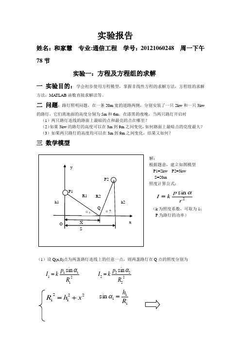
在漆黑的夜晚,当两只路灯开启时 (1)两只路灯连线的路面上最暗的点和最亮的点在哪里? (2)如果3kw 的路灯的高度可以在3m 到9m 之间变化,如何路面上最暗点的亮度最大? (3)如果两只路灯的高度均可以在3m 到9m 之间变化,结果又如何?三 数学模型解:根据题意,建立如图模型P1=2kw P2=3kw S=20m 照度计算公式:2sin r p k I α= (k 为照度系数,可取为1;P 为路灯的功率)(1)设Q(x,0)点为两盏路灯连线上的任意一点,则两盏路灯在Q 点的照度分别为21111sin R p k I α= 22222sin R p k I α=22121x h R += 111sin R h =α22222)(x s h R -+= 222sin R h =αQ 点的照度:3232322222322111))20(36(18)25(10))((()(()(x x x s h h P x h h P x I -+++=-+++=要求最暗点和最亮点,即为求函数I(x)的最大值和最小值,所以应先求出函数的极值点5252522222522111'))20(36()20(54)25(30))(()(3)(3)(x x x x x s h x s h P x h x h P x I -+-++-=-+-++-=算法与编程利用MATLAB 求得0)('=x I 时x 的值代码:s=solve('(-30*x)/((25+x^2)^(5/2))+(54*(20-x))/((36+(20-x)^2)^(5/2))'); s1=vpa(s,8); s1计算结果运行结果: s1 =19.97669581 9.338299136 8.538304309-11.61579012*i .2848997038e-1 8.538304309+11.61579012*i因为x>=0,选取出有效的x 值后,利用MATLAB 求出对应的I(x)的值,如下表:综上,x=9.33m 时,为最暗点;x=19.97m 时,为最亮点。
数学建模课后答案
数学建模课后答案数学建模课后答案【篇一:《数学模型》习题解答】t>1.学校共1000名学生,235人住在a宿舍,333人住在b宿舍,432人住在c宿舍.学生们要组织一个10人的委员会,试用下列办法分配各宿舍的委员数:(1). 按比例分配取整数的名额后,剩下的名额按惯例分给小数部分较大者; (2). 1中的q值方法;(3).d’hondt方法:将a、b、c各宿舍的人数用正整数n=1,2,3,??相除,其商数如下表:将所得商数从大到小取前10个(10为席位数),在数字下标以横线,表中a、b、c行有横线的数分别为2,3,5,这就是3个宿舍分配的席位.你能解释这种方法的道理吗?如果委员会从10个人增至15人,用以上3种方法再分配名额,将3种方法两次分配的结果列表比较.解:先考虑n=10的分配方案,p1?235,p2?333,p3?432,方法一(按比例分配)第二章(1)(2008年9月16日)pi?13i1000.q1?p1npi?132.35,q2?p2nipi?133.33, q3?p3nipi?134.32i分配结果为: n1?3, n2?3, n3?4 方法二(q值方法)9个席位的分配结果(可用按比例分配)为:n1?2,n2?3, n3?4第10个席位:计算q值为235233324322q1??9204.17, q2??9240.75, q3??9331.22?33?44?5q3最大,第10个席位应给c.分配结果为 n1?2,n2?3,n3?5方法三(d’hondt方法)此方法的分配结果为:n1?2,n2?3,n3?5此方法的道理是:记pi和ni为各宿舍的人数和席位(i=1,2,3代表a、b、c宿舍).pi是ni每席位代表的人数,取ni?1,2,?,从而得到的pip中选较大者,可使对所有的i,i尽量接近. nini再考虑n?15的分配方案,类似地可得名额分配结果.现将3种方法两次分配的结果列表如下:2.试用微积分方法,建立录像带记数器读数n与转过时间的数学模型. 解:设录像带记数器读数为n时,录像带转过时间为t.其模型的假设见课本.考虑t到t??t时间内录像带缠绕在右轮盘上的长度,可得vdt?(r?wkn)2?kdn,两边积分,得tvdt?2?k?(r?wkn)dnn2?rk?wk22n22vv《数学模型》作业解答第二章(2)(2008年10月9日)15.速度为v的风吹在迎风面积为s的风车上,空气密度是? ,用量纲分析方法确定风车获得的功率p与v、s、?的关系.解: 设p、v、s、?的关系为f(p,v,s,?)?0,其量纲表达式为: [p]=mlt 23, [v]=lt1,[s]=l,[?]=ml,这里l,m,t是基本量纲.2?3量纲矩阵为:1?2?10a=?3?1(p)(v)齐次线性方程组为:2?3?(l)01??(m) 00??(t)(s)(??2y1?y2?2y3?3y4?0y1?y4?03y?y?012?它的基本解为y?(?1,3,1,1) 由量纲pi定理得p?1v3s1?1,?p??v3s1?1 ,其中?是无量纲常数.16.雨滴的速度v与空气密度?、粘滞系数?和重力加速度g有关,其中粘滞系数的定义是:运动物体在流体中受的摩擦力与速度梯度和接触面积的乘积成正比,比例系数为粘滞系数,用量纲分析方法给出速度v的表达式.解:设v,?,?,g 的关系为f(v,?,?,g)=0.其量纲表达式为[v]=lmt,[?]=lmt,0-1-3[?]=mlt(ltl)l=mlltt=lmt,[g]=lmt,其中l,m,t是基本量纲.-2-1-1-1-2-2-2-1-10-2量纲矩阵为1?3?11?(l)?0?(m)110?a=? ???10?1?2(t)??(v)(?)(?)(g)齐次线性方程组ay=0 ,即y1-3y2-y3?y4?0?0 ?y2?y3-y-y-2y?034?1的基本解为y=(-3 ,-1 ,1 ,1) 由量纲pi定理得*v?3??1?g. ?v??3g,其中?是无量纲常数. ?16.雨滴的速度v与空气密度?、粘滞系数?、特征尺寸?和重力加速度g有关,其中粘滞系数的定义是:运动物体在流体中受的摩擦力与速度梯度和接触面积的乘积成正比,比例系数为粘滞系数,用量纲分析方法给出速度v的表达式.解:设v,?,?,?,g 的关系为f(v,?,?,?,g)?0.其量纲表达式为[v]=lmt,[?]=lmt,[?]=mlt(ltl)l=mlltt=lmt,[?]=lm0t0 ,[g]=lmt0-1-3-2-1-1-1-2-2-2-1-10-2其中l,m,t是基本量纲. 量纲矩阵为1?0a=1(v)齐次线性方程组ay=0 即(l)?(m)?00?1?2?(t)?(?)(?)(?)(g)1?3?10111y1?y2?3y3?y4?y5?0?y3?y4?0 ?y1?y4?2y5?0?的基本解为11?y?(1,?,0,0,?)?12231?y2?(0,?,?1,1,?)22?得到两个相互独立的无量纲量1?v??1/2g?1/23/2?1?1/2g??2??即 v?1) g?1,?3/2?g1/2??1??2?1. 由?(?1,?2)?0 , 得 ?1??(?2g?(?3/2?g1/2??1) , 其中?是未定函数.20.考察阻尼摆的周期,即在单摆运动中考虑阻力,并设阻力与摆的速度成正比.给出周期的表达式,然后讨论物理模拟的比例模型,即怎样由模型摆的周期计算原型摆的周期. 解:设阻尼摆周期t,摆长l, 质量m,重力加速度g,阻力系数k的关系为f(t,l,m,g,k)?0其量纲表达式为:[t]?l0m0t,[l]?lm0t0,[m]?l0mt0,[g]?lm0t?2,[k]?[f][v]?1?mlt?2(lt 1 )1l0mt?1,其中l,m,t是基本量纲.量纲矩阵为0?0a=1(t)?(l)?(m)?00?2?1??(t)(l)(m)(g)(k)10011001齐次线性方程组y2?y4?0??y3?y5?0 ?y?2y?y?045?1的基本解为11?y?(1,?,0,,0)?122 ?11y2?(0,,?1,?,1)22?得到两个相互独立的无量纲量tl?1/2g1/2??11/2?1?1/2lmgk??2∴t?kl1/2l1, ?1??(?2), ?2?gmg1/2∴t?lkl1/2(1/2) ,其中?是未定函数 . gmg考虑物理模拟的比例模型,设g和k不变,记模型和原型摆的周期、摆长、质量分别为t,t;l?kl?1/2l,l;m,m. 又t() 1/2gm?g当无量纲量m?l?t?l?gl?时,就有 ?.mltgll《数学模型》作业解答第三章1(2008年10月14日)1. 在3.1节存贮模型的总费用中增加购买货物本身的费用,重新确定最优订货周期和订货批量.证明在不允许缺货模型中结果与原来的一样,而在允许缺货模型中最优订货周期和订货批量都比原来结果减少.解:设购买单位重量货物的费用为k,其它假设及符号约定同课本.10 对于不允许缺货模型,每天平均费用为:【篇二:数学建模习题答案】t>中国地质大学能源学院华文静1.在稳定的椅子问题中,如设椅子的四脚连线呈长方形,结论如何?解:模型假设(1)椅子四条腿一样长,椅脚与地面接触处视为一点,四脚的连线呈长方形(2)地面高度是连续变化的,沿任何方向都不会出现间断(没有像台阶那样的情况),即从数学角度来看,地面是连续曲面。
数学建模竞赛 参考答案

数学建模竞赛参考答案数学建模竞赛参考答案数学建模竞赛是一项旨在培养学生数学建模能力和创新思维的竞赛活动。
参赛者需要在规定的时间内,针对给定的问题,运用数学知识和方法进行建模、分析和求解。
本文将为大家提供一些数学建模竞赛的参考答案,希望对参赛者有所帮助。
一、问题一:汽车油耗模型该问题要求建立一个汽车油耗模型,预测在不同的驾驶条件下,汽车的油耗情况。
首先,我们需要收集一些相关的数据,如汽车的型号、发动机排量、行驶里程、驾驶时间、驾驶速度等。
然后,我们可以使用多元线性回归模型来建立汽车油耗模型。
模型的建立如下:油耗= β0 + β1 * 发动机排量+ β2 * 行驶里程+ β3 * 驾驶时间+ β4 * 驾驶速度其中,β0、β1、β2、β3、β4为待求系数。
我们可以使用最小二乘法来估计这些系数。
通过对收集到的数据进行拟合,可以得到最优的系数估计值,并进一步预测不同驾驶条件下的汽车油耗情况。
二、问题二:物流配送路径规划该问题要求设计一个物流配送路径规划模型,以最小化配送成本和时间。
首先,我们需要收集一些相关的数据,如物流中心的位置、客户的位置、货物的重量和体积、道路交通情况等。
然后,我们可以使用网络流模型来建立物流配送路径规划模型。
模型的建立如下:目标函数:最小化总配送成本和时间约束条件:1. 每个客户都必须被配送到,并且每个物流中心只能配送给特定的客户。
2. 配送路径必须满足道路交通规则和限制条件。
3. 货物的重量和体积必须满足配送车辆的载重和容量限制。
我们可以使用线性规划或整数规划方法来求解该模型。
通过对收集到的数据进行建模和求解,可以得到最优的物流配送路径规划方案,以实现最小化成本和时间的目标。
三、问题三:疫情传播模型该问题要求建立一个疫情传播模型,预测疫情在不同地区的传播情况。
首先,我们需要收集一些相关的数据,如人口数量、人口流动情况、疫情传染率、潜伏期、治愈率等。
然后,我们可以使用传染病传播模型来建立疫情传播模型。
数学建模姚云飞第二版课后答案

数学建模姚云飞第二版课后答案1、向量与向量共线的充分必要条件是()[单选题] *A、两者方向相同B、两者方向相同C、其中有一个为零向量D、以上三个条件之一成立(正确答案)2、13.设x∈R,则“x3(x的立方)>8”是“|x|>2”的( ) [单选题] *A.充分而不必要条件(正确答案)B.必要而不充分条件C.充要条件D.既不充分也不必要条件3、19、如果点M是第三象限内的整数点,那么点M的坐标是()[单选题] *(-2,-1)(-2,-2)(-3,-1)(正确答案)(-3,-2)4、29、将点A(3,-4)平移到点B(-3,4)的平移方法有()[单选题] *A.仅1种B.2种C.3种D.无数多种(正确答案)5、一个直二面角内的一点到两个面的距离分别是3cm和4 cm ,求这个点到棱的距离为()[单选题] *A、25cmB、26cmC、5cm(正确答案)D、12cm6、若(m-3)+(4-2m)i为实数,那么实数m的值为()[单选题] *A、3B、4(正确答案)C、-2D、-37、23、在直角坐标平面内有点A,B,C,D,那么四边形ABCD的面积等于()[单选题]A. 1B. 2C. 4(正确答案)D. 2.58、9.点(-3,4)到y轴的距离是()[单选题] * A.3(正确答案)B.4C.-3D.-49、计算的结果是( ) [单选题] *A. -p2?(正确答案)B. p2?C. -p1?D. p1?10、下列说法正确的是()[单选题] *A、任何直线都有倾斜角(正确答案)B、任何直线都有倾斜角C、直线倾斜角越大斜率就越大D、直线与X轴平行则斜率不存在11、4、已知直角三角形的直角边边长分别是方程x2-14x+48=0的两个根,则此三角形的第三边是()[单选题] *A、6B、10(正确答案)C、8D、212、椭圆的离心率一定()[单选题] *A、等于1B、等于2(正确答案)C、大于1D、等于013、7.一条东西走向的道路上,小明向西走米,记作“米”,如果他向东走了米,则可记作()[单选题] *A-2米B-7米C-3米D+7米(正确答案)14、? 是第()象限的角[单选题] *A. 一(正确答案)B. 二C. 三D. 四15、9.下列说法中正确的是()[单选题] *A.正分数和负分数统称为分数(正确答案)B.正整数、负整数统称为整数C.零既可以是正整数,也可以是负整数D.一个有理数不是正数就是负数16、8.如果直角三角形的三条边为2,4,a,那么a的取值可以有()[单选题] *A. 0个B. 1个C. 2个D. 3个(正确答案)17、下列表示正确的是()[单选题] *A、0={0}B、0={1}C、{x|x2 =1}={1,-1}(正确答案)D、0∈φ18、9. 如图,在平面直角坐标系中,正方形ABCD的边长为2,点A坐标为(-2,1),沿某一方向平移后点A1的坐标为(4,2),则点C1的坐标为()[单选题]*A、(2,3)B、(2,4)(正确答案)C、(3,4)D、(3,3)19、若m·23=2?,则m等于[单选题] *A. 2B. 4C. 6D. 8(正确答案)20、1.计算-20+19等于()[单选题] *A.39B.-1(正确答案)C.1D.3921、下列各对象可以组成集合的是()[单选题] *A、与1非常接近的全体实数B、与2非常接近的全体实数(正确答案)C、高一年级视力比较好的同学D、与无理数相差很小的全体实数22、若(x+m)(x2-3x+n)展开式中不含x2和x项,则m,n的值分别为( ) [单选题] *A. m=3,n=1B. m=3,n=-9C. m=3,n=9(正确答案)D. m=-3,n=923、38、如图,点C、D分别在BO、AO上,AC、BD相交于点E,若CO=DO,则再添加一个条件,仍不能证明△AOC≌△BOD的是()[单选题] *A.∠A=∠BB.AC=BD(正确答案)C.∠ADE=∠BCED.AD=BC24、下列计算正确的是()[单选题] *A. a2+a2=2a?B. 4x﹣9x+6x=1C. (﹣2x2y)3=﹣8x?y3(正确答案)D. a6÷a3=a225、下列各对象可以组成集合的是()[单选题] *A、与1非常接近的全体实数B、与2非常接近的全体实数(正确答案)C、高一年级视力比较好的同学D、与无理数相差很小的全体实数26、22.如果|x|=2,那么x=()[单选题] * A.2B.﹣2C.2或﹣2(正确答案)D.2或27、下列运算正确的是()[单选题] *A. a2?a3=a?B. (﹣a3)2=﹣a?C. (ab)2=ab2D. 2a3÷a=2a2(正确答案)28、北京、南京、上海三个民航站之间的直达航线,共有多少种不同的飞机票?()[单选题] *A、3B、4C、6(正确答案)D、1229、如果四条不共点的直线两两相交,那么这四条直线()[单选题] *A、必定在同一平面内B、必定在同一平面内C可能在同一平面内,也可能不在同一平面内(正确答案)D、无法判断30、40.若x+y=2,xy=﹣1,则(1﹣2x)(1﹣2y)的值是()[单选题] *A.﹣7(正确答案)B.﹣3C.1D.9。
数学建模课后习题答案
第一章 课后习题6.利用1.5节药物中毒施救模型确定对于孩子及成人服用氨茶碱能引起严重中毒和致命的最小剂量。
解:假设病人服用氨茶碱的总剂量为a ,由书中已建立的模型和假设得出肠胃中的药量为:)()0(mg M x =由于肠胃中药物向血液系统的转移率与药量)(t x 成正比,比例系数0>λ,得到微分方程M x x dtdx=-=)0(,λ (1) 原模型已假设0=t 时血液中药量无药物,则0)0(=y ,)(t y 的增长速度为x λ。
由于治疗而减少的速度与)(t y 本身成正比,比例系数0>μ,所以得到方程:0)0(,=-=y y x dtdyμλ (2) 方程(1)可转换为:tMe t x λ-=)(带入方程(2)可得:)()(t t e e M t y λμμλλ----=将01386=λ和1155.0=μ带入以上两方程,得:t Me t x 1386.0)(-= )(6)(13866.01155.0---=e e M t y t针对孩子求解,得:严重中毒时间及服用最小剂量:h t 876.7=,mg M 87.494=; 致命中毒时间及服用最小剂量:h t 876.7=,mg M 8.4694= 针对成人求解:严重中毒时间及服用最小剂量:h t 876.7=,mg M 83.945= 致命时间及服用最小剂量:h t 876.7=,mg M 74.1987=课后习题7.对于1.5节的模型,如果采用的是体外血液透析的办法,求解药物中毒施救模型的血液用药量的变化并作图。
解:已知血液透析法是自身排除率的6倍,所以639.06==μut e t x λ-=1100)(,x 为胃肠道中的药量,1386.0=λ )(6600)(t t e e t y λμ---=1386.0,639.0,5.236)2(,1100,2,====≥-=-λλλu z e x t uz x dtdzt 解得:()2,274.112275693.01386.0≥+=--t e e t z t t用matlab 画图:图中绿色线条代表采用体外血液透析血液中药物浓度的变化情况。
数学建模 建模答案.docx
programi :(1) function [accum, varargout] = CircularHough_Grd(img, radrange, varargin) %Detect circular shapes in a grayscale image. Resolve their center %positions and radii.%% [accum, circen, cirrad, dbg_LMmask] = CircularHough_Grd(% img, radrange, grdthres, fltr4LM_R, multirad, fltr4accum)% Circular Hough transform based on the gradient field of an image.% NOTE: Operates on grayscale images, NOT B/W bitmaps.% NO loops in the implementation of Circular Hough transform,% which means faster operation but at the same time larger% memory consumption.%%%%%%%%% INPUT: (img, radrange, grdthres, fltr4LM_R, multirad, fltr4accum) % % img: A 2-D grayscale image (NO B/W bitmap)%% radrange: The possible minimum and maximum radii of the circles% to be searched, in the format of% [minimum radius , maximum_radius] (unit: pixels)% **NOTE**: A smaller range saves computational time and% memory.%% grdthres: (Optional, default is 10, must be non-negative)% The algorithm is based on the gradient field of the% input image. A thresholding on the gradient magnitude% is performed before the voting process of the Circular% Hough transform to remove the Uniform intensity'% (sort-of) image background from the voting process.% In other words, pixels with gradient magnitudes smaller% than 'grdthres' are NOT considered in the computation.% **NOTE**: The default parameter value is chosen for% images with a maximum intensity close to 255. For cases% with dramatically different maximum intensities, e.g.% 10-bit bitmaps in stead of the assumed 8-bit, the default% value can NOT be used. A value of 4% to 10% of the maximum% intensity may work for general cases.%% fltr4LM_R: (Optional, default is 8, minimum is 3)% The radius of the filter used in the search of local% maxima in the accumulation array. To detect circles whose% shapes are less perfect, the radius of the filter needs% to be set larger.%% multirad: (Optional, default is 0.5)% In case of concentric circles, multiple radii may be% detected corresponding to a single center position. This% argument sets the tolerance of picking up the likely% radii values. It ranges from 0.1 to 1, where 0.1% corresponds to the largest tolerance, meaning more radii % values will be detected, and 1 corresponds to the smallest % tolerance, in which case only the "principal" radius will% be picked up.%% fltr4accum: (Optional. A default filter will be used if not given)% Filter used to smooth the accumulation array. Depending % on the image and the parameter settings, the accumulation % array built has different noise level and noise pattern% (e.g. noise frequencies). The filter should be set to an% appropriately size such that ifs able to suppress the% dominant noise frequency.%%%%%%%%% OUTPUT: [accum, circen, cirrad, dbg_LMmask]%% accum: The result accumulation array from the Circular Hough% transform. The accumulation array has the same dimension % as the input image.%% circen: (Optional)% Center positions of the circles detected. Is a N-by-2% matrix with each row contains the (x, y) positions% of a circle. For concentric circles (with the same center% position), say k of them, the same center position will% appear k times in the matrix.%% cirrad: (Optional)% Estimated radii of the circles detected. Is a N-by-1% column vector with a one-to-one correspondance to the% output tircen*. A value 0 for the radius indicates a% failed detection of the circle's radius.%% dbg_LMmask: (Optional, for debugging purpose)% Mask from the search of local maxima in the accumulation % array.%%%%%%%%%% EXAMPLE #0:% rawimg = imread('TestImg_CHT_a2.bmp');% tic;% [accum, circen, cirrad] = CircularHough_Grd(rawimg, [15 60]);% toe;% figure(l); imagesc(accum); axis image;% title(,Accumulation Array from Circular Hough Transfbrm,);% figure(2); imagesc(rawimg); colormap(,gray,); axis image;% hold on;% plot(circen(:,l), circen(:,2), *r+');% for k = 1 : size(circen, 1),% DrawCircle(circen(k, 1), circen(k,2), cirrad(k), 32,,b」);% end% hold off;% title([*Raw Image with Circles Detected% '(center positions and radii marked)*]);% figure(3); surf(accum, 'EdgeColoF, hone'); axis ij;% title('3-D View of the Accumulation Array*);%% COMMENTS ON EXAMPLE #0:% Kind of an easy case to handle. To detect circles in the image whose% radii range from 15 to 60. Default values for arguments 'grdthres',% 'fltr4LM_R', 'multirad* and ,fltr4accum, are used.%%%%%%%%%% EXAMPLE #1:% rawimg = imread('TestImg_CHT_a3.bmp');% tic;% [accum, circen, cirrad] = CircularHough_Grd(rawimg, [15 60], 10, 20);% toe;% figure(l); imagesc(accum); axis image;% title(,Accumulation Array from Circular Hough Transfbrm,);% figure(2); imagesc(rawimg); colormap('gray'); axis image;% hold on;% plot(circen(:,l), circen(:,2), T+');% for k = 1 : size(circen, 1),% DrawCircle(circen(k, 1), circen(k,2), cirrad(k), 32, 'b-');% end% hold off;% title([*Raw Image with Circles Detected% '(center positions and radii marked)*]);% figure(3); surf(accum, 'EdgeColoF, hone'); axis ij;% title(*3-D View of the Accumulation Array*);%% COMMENTS ON EXAMPLE #1:% The shapes in the raw image are not very good circles. As a result,% the profile of the peaks in the accumulation array are kind of% 'stumpy', which can be seen clearly from the 3-D view of the% accumulation array, (As a comparison, please see the sharp peaks in % the accumulation array in example #0) To extract the peak positions % nicely, a value of 20 (default is 8) is used for argument 'fltr4LM_R', % which is the radius of the filter used in the search of peaks.%%%%%%%%%% EXAMPLE #2:% rawimg = imread(,TestImg_CHT_b3 .bmp1);% fltr4img = [1 1 1 1 1; 1 2 2 2 1; 1 2 4 2 1; 1 2 2 2 1; 1 1 1 1 1];% fltr4img = fltr4img / sum(fltr4img(:));% imgfltrd = filter2( fltr4img , rawimg );% tic;% [accum, circen, cirrad] = CircularHough_Grd(imgfltrd, [15 80], 8, 10); % toe;% figure(l); imagesc(accum); axis image;% title(,Accumulation Array from Circular Hough Transfbrm,);% figure(2); imagesc(rawimg); colormap('gray'); axis image;% hold on;% plot(circen(:,l), circen(:,2), T+');% for k = 1 : size(circen, 1),% DrawCircle(circen(k, 1), circen(k,2), cirrad(k), 32, 'b-');% end% hold off;% title([*Raw Image with Circles Detected% '(center positions and radii marked)*]);%% COMMENTS ON EXAMPLE #2:% The circles in the raw image have small scale irregularities along % the edges, which could lead to an accumulation array that is bad for % local maxima detection. A 5-by-5 filter is used to smooth out the % small scale irregularities. A blurred image is actually good for the % algorithm implemented here which is based on the image's gradient % field.%%%%%%%%%% EXAMPLE #3:% rawimg = imread('TestImg_CHT_c3.bmp');% fltr4img = [1 1 1 1 1; 1 2 2 2 1; 1 2 4 2 1; 1 2 2 2 1; 1 1 1 1 1];% fltr4img = fltr4img / sum(fltr4img(:));% imgfltrd = filter2( fltr4img , rawimg );% tic;% [accum, circen, cirrad]=...% CircularHough_Grd(imgfltrd, [15 105], 8, 10, 0.7);% toe;% figure(l); imagesc(accum); axis image;% figure(2); imagesc(rawimg); colormap(,gray,); axis image;% hold on;% plot(circen(:,l), circen(:,2), *r+');% for k = 1 : size(circen, 1),% DrawCircle(circen(k, 1), circen(k,2), cirrad(k), 32,,b」);% end% hold off;% title([*Raw Image with Circles Detected% '(center positions and radii marked)*]);%% COMMENTS ON EXAMPLE #3:% Similar to example #2, a filtering before circle detection works for% noisy image too. 'multirad* is set to 0.7 to eliminate the false% detections of the circles* radii.%%%%%%%%%% BUG REPORT:% This is a beta version. Please send your bug reports, comments and% suggestions to pengtao@ . Thanks.%%%%%%%%%%% INTERNAL PARAMETERS:% The INPUT arguments are just part of the parameters that are used by% the circle detection algorithm implemented here. Variables in the code% with a prefix ,prm_, in the name are the parameters that control the% judging criteria and the behavior of the algorithm. Default values for% these parameters can hardly work for all circumstances. Therefore, at% occasions, the values of these INTERNAL PARAMETERS (parameters that% are NOT exposed as input arguments) need to be fine-tuned to make% the circle detection work as expected.% The following example shows how changing an internal parameter could% influence the detection result.% 1. Change the value of the internal parameter 'prm LM LoBndRa* to 0.4% (default is 0.2)% 2. Run the following matlab code:% fltr4accum = [1 2 1; 2 6 2; 1 2 1];% fltr4accum = fltr4accum / sum(fltr4accum(:));% rawimg = imread(,Frame_0_0022jportion.jpg,);% tic;% [accum, circen] = CircularHough_Grd(rawimg,...% [4 14], 10, 4, 0.5, fltr4accum);% toe;% figure(l); imagesc(accum); axis image;% title(*Accumulation Array from Circular Hough Transform*);% figure(2); imagesc(rawimg); colormap(,gray,); axis image;% hold on; plot(circen(:,l), circen(:,2), "); hold off;% title('Raw Image with Circles Detected (center positions marked)*);% 3. See how different values of the parameter 'prm LM LoBndRa* could % influence the result.% Author: Tao Peng% Department of Mechanical Engineering% University of Maryland, College Park, Maryland 20742, USA% pengtao@% Version: Beta Revision: Mar. 07, 2007%%%%%%%% Arguments and parameters %%%%%%%%%%%%%%%%%%%%%%%%%%%%%%%%%%%% Validation of argumentsif ndims(img)〜=2 || 〜isnumeric(img),error(*CircularHough_Grd: "img" has to be 2 dimensionaf);endif 〜all(size(img) >= 32),erro^'CircularHough Grd: "img" has to be larger than 32-by-32');endif numel(radrange)〜=2 || -isnumeric(radrange),error([*CircularHough_Grd: "radrange" has to be \ ...'a two-element vector1]);endprm_r_range = sort(max( [0,0;radrange( 1 ),radrange(2)]));% Parameters (default values)prmgrdthres = 10;prmfltrLMR = 8;prmmultirad = 0.5;funccompucen = true;funccompuradii = true;% Validation of argumentsvapgrdthres = 1;if nargin > (1 + vap_grdthres),if isnumeric(varargin{vap grdthres}) && ...varargin(vap grdthres} (1) >= 0,prm_grdthres = varargin {vapgrdthres} (1);elseerror(['CircularHough_Grd: "grdthres" has to be'a non-negative number1]);endendvap_fltr4LM = 2; % filter for the search of local maximaif nargin > (1 + vap_fltr4LM),if isnumeric(varargin{vap_fltr4LM}) && varargin{vap_fltr4LM}(1) >= 3, prmfltrLMR = varargin{vap_fltr4LM} (1);elseerror([,CircularHough_Grd: n fltr4LM_R n has to belarger than or equal to 3']);endendvap_multirad = 3;if nargin > (1 + vap multirad),if isnumeric(varargin{vap_multirad}) && ...varargin{vap multirad}(1) >= 0.1 && ...varargin {vap multirad} (1) <= 1,prmmultirad = varargin {vap_mul tirad} (1);elseerror(['CircularHough_Grd: "multirad" has to be'within the range [0.1, 1]*]);endendvap_fltr4accum = 4; % filter for smoothing the accumulation arrayif nargin > (1 + vap_fltr4accum),if isnumeric(varargin{vap_fltr4accum}) && ...ndims(varargin{vap_fltr4accum}) == 2 && ...all(size(varargin {vap_fltr4accum}) >= 3),fltr4accum = varargin {vap_fltr4accum};elseerror(['CircularHough_Grd: n fltr4accum n has to be \ ...*a 2-D matrix with a minimum size of 3-by-3']);endelse% Default filter (5-by-5)fltr4accum = ones(5,5);fltr4accum(2:4,2:4) = 2;fltr4accum(3,3) = 6;end func_compu_cen = (nargout > 1 );func_compu_radii = (nargout > 2 );% Reserved parametersdbg on = false; % debug information dbgbfigno = 4;if nargout > 3, dbg on = true; end%%%%%%%% Buildingaccumulation array %%%%%%%%%%%%%%%%%%%%%%%%%%%%%%%%% Convert the image to single if it is not of% class float (single or double) img_is_double = isa(img, double');if ~(img_is_double || isa(img, 'single')),imgf = single(img);end% Compute the gradient and the magnitude of gradientif img_is_double,[grdx, grdy] = gradient(img);else[grdx, grdy] = gradient(imgf);endgrdmag = sqrt(grdx.A2 + grdy.A2);% Get the linear indices, as well as the subscripts, of the pixels% whose gradient magnitudes are larger than the given threshold grdmasklin = find(grdmag > prm_grdthres);[grdmask_ldxl, grdmask_IdxJ] = ind2sub(size(grdmag), grdmasklin);% Compute the linear indices (as well as the subscripts) of% all the votings to the accumulation array.% The Matlab function 'accumarray* accepts only double variable, % so all indices are forced into double at this point.% A row in matrix ,lin2accum_aJ, contains the J indices (into the % accumulation array) of all the votings that are introduced by a % same pixel in the image. Similarly with matrix linZaccum aP. rr_41inaccum = double( prm_r_range );linaccum_dr = [ (-rr_41inaccum(2) + 0.5) : -rr_41inaccum(l),... (rr_41inaccum(l) + 0.5) : rr_41inaccum(2)];lin2accum_aJ = floor(...double(grdx(grdmasklin)./grdmag(grdmasklin)) * linaccum_dr + ...repmat( double(grdmask_IdxJ)+0.5 , [ 1 ,length(linaccum_dr)])...);lin2accum_al = floor(...double(grdy(grdmasklin)./grdmag(grdmasklin)) * linaccum dr + ...repmat( double(grdmask_IdxI)+0.5 , [1 ,length(linaccum_dr)])...);% Clip the votings that are out of the accumulation arraymask_valid_a J al =...lin2accum_aJ > 0 & lin2accum_aJ < (size(grdmag,2) + 1) & ...Iin2accum_al > 0 & lin2accum_al < (size(grdmag,l) + 1);mask_valid_aJaI_reverse =〜mask_valid_aJaI;lin2accum_aJ = lin2accum_aJ .* maskvalida J al + maskvalidaJ alreverse;lin2accum_al = lin2accum_al .* mask_valid_aJaI + mask_valid_aJaI_reverse;clear mask_valid_aJ alre verse;% Linear indices (of the votings) into the accumulation arraylin2accum = sub2ind( size(grdmag), lin2accum_al, lin2accum_aJ );lin2accum_size = size( lin2accum );lin2accum = reshape( lin2accum, [numel(lin2accum),l]);clear lin2accum_al lin2accum_aJ;% Weights of the votings, currently using the gradient maginitudes% but in fact any scheme can be used (application dependent)weight4accum =...repmat( double(grdmag(grdmasklin)) , [lin2accum_size(2), 1 ]) .* ...mask_valid_aJ al(:);clear mask_valid_aJaI;% Build the accumulation array using Matlab function 'accumarray'accum = accumarray( lin2accum , weight4accum );accum = [ accum ; zeros( numel(grdmag) - numel(accum), 1 )];accum = reshape( accum, size(grdmag));%%%%%%%% Locating local maxima in the accumulation array %%%%%%%%%%%%% Stop if no need to locate the center positions of circlesif ~func_compu_cen,return;endclear lin2accum weight4accum;% Parameters to locate the local maxima in the accumulation array% — Segmentation of 'accum' before locating LM prmuseaoi = true;prm_aoithres_s = 2;prm aoiminsize = floor(min([ min(size(accum)) * 0.25,... prm_r_range(2) * 1.5 ]));% — Filter for searching for local maxima prmfltrLMs = 1.35;prm fltrLM r = ceil( prm fltrLM R * 0.6 );prm fltrLM npix = max([ 6, ceil((prm_fltrLM_R/2)A 1.8)]);% — Lower bound of the intensity of local maximaprm LM LoBndRa = 0.2; % minimum ratio of LM to the max of'accum'% Smooth the accumulation arrayfltr4accum = fltr4accum / sum(fltr4accum(:));accum = filter2( fltr4accum, accum );% Select a number of Areas-Of^Interest from the accumulation array if prmuseaoi, % Threshold value for 'accum1prm_llm_thresl = prm_grdthres * prm_aoithres_s;% Thresholding over the accumulation array accummask = ( accum > prm llm thres 1 );% Segmentation over the mask[accumlabel, accum nRgn] = bwlabel( accummask, 8 );% Select AOIs from segmented regionsaccumAOI = ones(0,4);for k = 1 : accum nRgn,accumrgn lin = find( accumlabel = k);[accumrgn_ldxl, accumrgn_IdxJ]=...ind2sub( size(accumlabel), accumrgn lin);rgn top = min( accumrgn ldxl);rgn bottom = max( accumrgn_ldxl);rgn left = min( accumrgn ldxJ );rgn_right = max( accumrgn ldxJ );% The AOIs selected must satisfy a minimum sizeif ((rgn_right - rgn_left + 1) >= prm_aoiminsize && ...(rgn_bottom - rgn top + 1) >= prm aoiminsize ),accumAOI = [ accumAOI;...rgn top, rgn bottom, rgn left, rgn right ];endendelse% Whole accumulation array as the one AOIaccumAOI = [1, size(accum,l), 1, size(accum,2)];end% Thresholding of 'accum' by a lower boundprm LM LoBnd = max(accum(:)) * prm LM LoBndRa;% Build the filter for searching for local maxima fltr4LM = zeros(2 * prm_fltrLM_R + 1);[mesh4fLM_x, mesh4fLM_y] = meshgrid(-prm_fltrLM_R : prm fltrLM R);mesh4fLM_r = sqrt( mesh4fLM_x.A2 + mesh4fLM_y.A2 );fltr4LM_mask =...(mesh4fLM_r > prm_fltrLM_r & mesh4fLM_r <= prm fltrLM R );fltr4LM = fltr4LMfltr4LM_mask * (prm fltrLM s / sum(fltr4LM_mask(:)));if prm_fltrLM_R >= 4,fltr4LM_mask = ( mesh4fLM_r < (prm_fltrLM_r - 1));elsefltr4LM_mask = ( mesh4fLM_r < prm fltrLM r );endfltr4LM = fltr4LM + fltr4LM mask / sum(fltr4LM_mask(:));% **** Debug code (begin)if dbg_on,dbg_LMmask = zeros(size(accum));end% **** Debug code (end)% For each of the AOIs selected, locate the local maximacircen = zeros(0,2);fbrk = 1 : size(accumAOI, 1),aoi = accumAOI(k,:); % just for referencing convenience% Thresholding of 'accum* by a lower boundaccumaoi_LBMask =...(accum(aoi(l):aoi(2), aoi(3):aoi(4)) > prm LM LoBnd );% Apply the local maxima filtercandLM = conv2( accum(aoi( 1):aoi(2), aoi(3):aoi(4)),...fltr4LM, 'same*);candLM mask = ( candLM > 0 );% Clear the margins of 'candLM mask*candLM_mask([l :prm_fltrLM_R, (end-prm_fltrLM_R+l):end], :) = 0;candLM mask(:, [l:prm_fltrLM_R, (end-prm_fltrLM_R+l):end]) = 0;% **** Debug code (begin)if dbg_on,dbg_LMmask(aoi( 1 ):aoi(2), aoi(3):aoi(4))=...dbg_LMmask(aoi( 1 ):aoi(2), aoi(3):aoi(4)) + ...accumaoi LBMask + 2 * candLM mask;end% **** Debug code (end)% Group the local maxima candidates by adjacency, compute the% centroid position for each group and take that as the center% of one circle detected[candLM label, candLM nRgn] = bwlabel( candLM_mask, 8 );fbr ilabel = 1 : candLM nRgn,% Indices (to current AOI) of the pixels in the groupcandgrp masklin = find( candLM label == ilabel);[candgrp_ldxl, candgrp_IdxJ]=...ind2sub( size(candLM label), candgrp masklin );% Indices (to 'accum') of the pixels in the groupcandgrp_ldxl = candgrp_ldxl + ( aoi(l) - 1 );candgrp IdxJ = candgrp IdxJ + ( aoi(3) - 1 );candgrp_idx2acm =...sub2ind( size(accum) , candgrp ldxl, candgrp IdxJ );% Minimum number of qulified pixels in the groupif sum(accumaoi_LBMask(candgrp_masklin)) < prm_fltrLM_npix, continue;end% Compute the centroid positioncandgrp_acmsum = sum( accum(candgrp_idx2acm));cc_x = sum( candgrp IdxJ .* accum(candgrp_idx2acm) ) / ...candgrpacmsum;cc_y = sum( candgrp_ldxl .* accum(candgrp_idx2acm) ) / ...candgrpacmsum;circen = [circen; cc_x, cc_y];endend% **** Debug code (begin)if dbg_on,figure(dbg bfigno); imagesc(dbg LMmask); axis image;title(*Generated map of local maxima1);if size(accumAOI, 1) == 1,figure(dbg_bfigno+1);surf(candLM, 'EdgeColor1, hone'); axis ij;title(,Accumulation array after local maximum filtering*);endend% **** Debug code (end)%%%%%%%% Estimation of the Radii of Circles %%%%%%%%%%%%% Stop if no need to estimate the radii of circlesif ~func_compu_radii,varargout{l} = circen;return;end% Parameters for the estimation of the radii of circlesfltr4SgnCv=[2 1 1];fltr4SgnCv = fltr4SgnCv / sum(fltr4SgnCv);% Find circle's radius using its signature curve cirrad = zeros( size(circen,l), 1 );for k = 1 : size(circen,l),% Neighborhood region of the circle for building the sgn. curve circen_round = round( circen(k,:));SCvR IO = circen_round(2) - prm_r_range(2) - 1;ifSCvR_IO<l,SCvR_I0= 1;endSCvRIl = circen_round(2) + prm_r_range(2) + 1;if SCvR Il > size(grdx,l),SCvRIl = size(grdx,l);endSCvR JO = circen round(l) - prm_r_range(2) - 1;ifSCvR_JO<l,SCvRJO = 1;endSCvRJ 1 = circenround(l) + prm_r_range(2) + 1;if SCvR Jl > size(grdx,2),SCvRJl = size(grdx,2);end% Build the sgn. curveSgnCvMat_dx = repmat( (SCvR J0:SCvR J 1) - circen(k,l),...[SCvRJl - SCvRJO +1,1]);SgnCvMat_dy = repmat( (SCvR_IO:SCvR_Il)' - circen(k,2),...[1 , SCvRJl - SCvRJO + 1]);SgnCvMat_r = sqrt( SgnCvMat dx .A2 + SgnCvMat_dy .A2 );SgnCvMatrpl = round(SgnCvMatr) + 1;f4SgnCv = abs(...double(grdx(SCvR_IO:SCvR_Il, SCvRJO:SCvRJ 1)) .* SgnCvMat_dx + ...double(grdy(SCvR_IO:SCvR Il, SCvR JO:SCvR J 1)) .* SgnCvMat dy...)./ SgnCvMat r;SgnCv = accumarray( SgnCvMat rp 1(:) , f4SgnCv(:));SgnCv_Cnt = accumarray( SgnCvMat rp 1 (:) , ones(numel(f4SgnCv), 1));SgnCv_Cnt = SgnCv_Cnt + (SgnCv_Cnt == 0);SgnCv = SgnCv ./ SgnCv_Cnt;% Suppress the undesired entries in the sgn. curve% ― Radii that correspond to short arcsSgnCv = SgnCv .* ( SgnCv_Cnt >= (pi/4 * [O:(numel(SgnCv_Cnt)-1 )]*));% ― Radii that are out of the given rangeSgnCv( 1 : (round(prm_r_range( 1))+1) ) = 0;SgnCv( (round(prm_r_range(2))+1) : end ) = 0;% Get rid of the zero radius entry in the arraySgnCv = SgnCv(2:end);% Smooth the sgn. curveSgnCv = filtfilt( fltr4SgnCv , [1] , SgnCv );% Get the maximum value in the sgn. curveSgnCv_max = max(SgnCv);if SgnCv_max <= 0,cirrad(k) = 0;continue;end% Find the local maxima in sgn. curve by 1st order derivatives% ― Mark the ascending edges in the sgn. curve as Is and% ― descending edges as OsSgnCv AscEdg = ( SgnCv(2:end) - SgnCv(l:(end-l)) ) > 0;% ― Mark the transition (ascending to descending) regionsSgnCv LMmask = [ 0; 0; SgnCv_AscEdg(l:(end-2)) ] & (〜SgnCv_AscEdg);SgnCv LMmask = SgnCvLMmask & [ SgnCv_LMmask(2:end); 0 ];% Incorporate the minimum value requirementSgnCvLMmask = SgnCvLMmask & ...(SgnCv(l:(end-l)) >= (prm_multirad * SgnCv_max));% Get the positions of the peaksSgnCv LMPos = sort( find(SgnCv_LMmask));% Save the detected radiiif isempty(SgnCvLMPos),cirrad(k) = 0;elsecirrad(k) = SgnCvLMPos(end);for i radii = (length(SgnCv LMPos) - 1) : -1 : 1,circen = [ circen; circen(k,:)];cirrad = [ cirrad; SgnCv_LMPos(i_radii)];endendend% Outputvarargout{l} = circen;varargout{2} = cirrad;if nargout > 3,varargout{3} = dbg_LMmask;endprograms:programs:2 function DrawCircle (x, y, r, nseg, S)% Draw a circle on the current figure using ploylines%% DrawCircle (x, y, r, nseg, S)% A simple function for drawing a circle on graph.%% INPUT: (x, y, r, nseg, S)% x, y: Center of the circle% r: Radius of the circle% nseg: Number of segments for the circle% S: Colors, plot symbols and line types%% OUTPUT: None%% BUG REPORT:% Please send your bug reports, comments and suggestions to% pengtao@glue. umd. edu . Thanks.% Author: Tao Peng% Department of Mechanical Engineering% University of Maryland, College Park, Maryland 20742, USA % pengtao@glue. umd. edu% Version: alpha Revision: Jan. 10, 2006theta = 0 : (2 * pi / nseg) : (2 * pi);pline_x 二r * cos(theta) + x;pline_y 二r * sin(theta) + y;plot (pline_x, pline_y, S);3function testiml二imread (' image 1. jpg');% rawimg = imread(,TestImg_CHT_c3. bmp J);rawimg=rgb2gray(iml);tic;[accum, circen, cirrad] = CircularHough_Grd(rawimg, [20 30], 5,50);circentoe;figure(1) ; imagesc(accum); axis image;title (J Accumulation Array from Circular Hough Transform,); figure (2) ; imagesc (rawimg) ; colormap (J gray,) ; axis image; hold on;plot (circen(:, 1), circen(:, 2), ' r+');for k = 1 : size (circen, 1),DrawCircle (circen (k, 1), circen (k, 2), cirrad (k), 32, ' b-'); end hold off; title(f Raw Image with Circles Detected ...'(center positions and radii marked)']);figure (3); surf(accum, ' EdgeColor,, ' none5); axis ij; title (J 3-D View of the Accumulation Array');附带图像image 1. jpg直接运行test.m即可得到上方的结果!当然方法是活的,只要合理即可行。
数学建模陈东彦版课后答案
数学建模陈东彦版课后答案篇一:数学建模承诺书我们仔细阅读了中国大学生数学建模竞赛的竞赛规则.我们完全明白,在竞赛开始后参赛队员不能以任何方式(包括电话、电子邮件、网上咨询等)与队外的任何人(包括指导教师)研究、讨论与赛题有关的问题。
我们知道,抄袭别人的成果是违反竞赛规则的, 如果引用别人的成果或其他公开的资料(包括网上查到的资料),必须按照规定的参考文献的表述方式在正文引用处和参考文献中明确列出。
我们郑重承诺,严格遵守竞赛规则,以保证竞赛的公正、公平性。
如有违反竞赛规则的行为,我们将受到严肃处理。
我们参赛选择的题号是(从A/B/C/D中选择一项填写):我们的参赛报名号为(如果赛区设置报名号的话):所属(请填写完整的全名):参赛队员 (打印并签名) :1.指导教师或指导教师组负责人 (打印并签名)日期: 2010 年 11 月 22 日赛区评阅编号(由赛区组委会评阅前进行编号):编号专用页赛区评阅编号(由赛区组委会评阅前进行编号):全国统一编号(由赛区组委会送交全国前编号):全国评阅编号(由全国组委会评阅前进行编号):对等高线图转化为三维地形图以及水的流向的探讨摘要:在等高线地形图上,根据等高线不同的弯曲形态,可以判读出地表形态的一般状况。
等高线呈封闭状时,高度是外低内高,则表示为凸地形(如山峰、山地、丘顶等);等高线高度是外高内低,则表示的是凹地形(如盆地、洼地等)。
等高线是曲线状时,等高线向高处弯曲的部分表示为山谷;等高线向低处凸出处为山脊。
数条高程不同的等高线相交一处时,该处的地形部位为陡崖,并在图上绘有陡崖图例。
由一对表示山谷与一对表示山脊的等高线组成的地形部位为鞍部。
等高线密集的地方表示该处坡度较陡;等高线稀疏的地方表示该处坡度较缓。
问题一:由等高线图转换为三维地形图有好多种方法,本文用坡度、坡向、等高线膨胀法以及建立空间直角坐标系的方法建立数学模型,把等高线图转化成三维地形图。
问题二:把地面无限细分为无限个单元格。
科学计算与数学建模智慧树知到课后章节答案2023年下中南大学
科学计算与数学建模智慧树知到课后章节答案2023年下中南大学中南大学第一章测试1.以下哪种误差可以完全避免?答案:过失误差2.关于误差的衡量,哪个是不准确的?答案:估计误差3.进行减法运算时,要尽量做到()?答案:避免相近的近似数相减4.算法的计算复杂性可以通过来衡量?答案:算法的时间复杂度5.在数学建模过程中,要遵循尽量采用 ( ) 的数学工具这一原则,以便更多人能了解和使用?答案:简单第二章测试1.若n+1个插值节点互不相同,则满足插值条件的n次插值多项式()?答案:唯一存在2.三次样条函数的插值条件中,最多可以插值于给定数据点的阶导数?答案:23.当要计算的节点x 靠近给定数据点终点xn时,选择公式比较合适?答案:Newton向后插值4.n+1 个点的插值多项式,其插值余项对f(x)一直求到()阶导数?答案:n+15.三次样条插值只需要插值节点位置即可。
答案:错第三章测试1.有4个不同节点的高斯求积公式的代数精度是答案:72.复合Simpson求积公式具几阶收敛性答案:33.答案:24.以下哪项不属于数值求积的必要性?答案:f(x)的不能用初等函数表示。
5.辛普森公式又名()?答案:抛物线公式第四章测试1.下面关于二分法的说法哪个错误的()?答案:只要步长足够小,用二分法可以求出方程的所有根。
2.二分法中求解非线性方程时,分割次数越多得出的根越精确?答案:错3.将化成的结果是唯一的?答案:错4.答案:(1)和(2)5.答案:第五章测试1.式Ax=b中,n阶矩阵A =(a ij)n×n为方程组的矩阵?答案:系数2.如果 L是单位下三角矩阵,U 为上三角矩阵,此时是三角分解称为克劳特(Crout)分解;若 L 是下三角矩阵,而 U 是单位上三角矩阵,则称三角分解为杜利特(Doolittle)分解?答案:错3.LU分解实质上是Gauss消去法的矩阵形式。
答案:对4.若n阶非奇异矩阵A的前n-1阶顺序主子式有的为0,则可以在A的左边或右边乘以初等矩阵,就将A的行或列的次序重新排列,使A的前n-1阶顺序主子式非0,从而可以进行三角分解?答案:对5.采用高斯消去法解方程组时, 小主元可能产生麻烦,故应避免采用绝对值小的主元素?答案:对第六章测试1.运用迭代法求解线性方程组时,原始系数矩阵在计算过程中始终不变?答案:对2.迭代法不适用于求解大型稀疏系数矩阵方程组?答案:错3.迭代法可以求解出线性方程组的解析解?答案:错4.答案:5.答案:第七章测试1.答案:p2.答案:1.00003.答案:对4.当 k=0 时,Adams内插法就是Euler法。
部分数学建模习题解答
第一章第5题一个男孩和一个女孩分别在离家2km和1km且方向相反的两所学校里上学,每天同时放学后分别以2km/h和1km/h的速度步行回家。
一只小狗以6km/h的速度由男孩奔向女孩,又从女孩处跑向跑回男孩处,如此往返的奔跑,直至回到家中。
问小狗总共奔波了多少路程?解:由于男孩、女孩与小狗跑的时间一样,所以把时间设为t,则有2t+1t=3,得到t=1h。
所以小狗跑了6km/h*1h=6km。
第一章10题一位探险家必须穿过一片宽度为800 km的沙漠,他仅有的交通工具是一辆每升汽油可行驶10km的吉普车.吉普车的油箱可装10升汽油。
另外吉普车上可携带8个可装5升汽油的油桶,也就是说,吉普车最多可带50升汽油(最多能在沙漠中连续行驶500 km)。
现假定在探险家出发地的汽油是无限充足的.问这位保险家应怎样设计他的旅行才能通过此沙漠?他要通过沙漠所需的汽油最少是多少升?为了穿越这片800km宽的沙漠,他总共需要行驶多少公里路程。
总共要花费多少升的汽油?思路:1、若沙漠只有500公里或者更短,这时很简单,一次搞定。
2、若沙漠有550km,怎么办?需要保证的是:车到了离沙漠终点还有500km的地方,能恰恰加满油且不会有多余。
方案可为:600-550=50,从起点处加5*3(升)=15升油,开出50km,设一加油站,存下5升,剩下5升刚好使得汽车返回起点。
再在起点处加满50升油,到加油站时,只乘45升了,把存放在那儿的5升油加上。
则可跑出沙漠。
(这样共加油15+50=65,总路程为150+500=650km)3、再看2的情况,符合这种情况的沙漠的最大距离是多少呢:答案是500*(1+1/3)公里。
即在起点准备100升油,第一次装50升,跑了500/3公里后存放50*1/3升油,然后返回起点,这时车里的油也正好用完,然后再在起点处装50升,跑了550/3公里后,车内剩下(50*2/3)升油,再加上存放的50*1/3升油,恰好为50升油,则可跑出沙漠。
- 1、下载文档前请自行甄别文档内容的完整性,平台不提供额外的编辑、内容补充、找答案等附加服务。
- 2、"仅部分预览"的文档,不可在线预览部分如存在完整性等问题,可反馈申请退款(可完整预览的文档不适用该条件!)。
- 3、如文档侵犯您的权益,请联系客服反馈,我们会尽快为您处理(人工客服工作时间:9:00-18:30)。
第一章
4.在1.3节“椅子能在不平的地面上放稳吗”的假设条件中,将四脚的连线呈正方形改为长方形,其余不变。
试构造模型并求解。
答:相邻两椅脚与地面距离之和分别定义为)()(a g a f 和。
f 和g 都是连续函数。
椅子在任何位置至少有三只脚着地,所以对于任意的a ,)()(a g a f 和中至少有一个不为零。
不妨设0)0(,0)0(g >=f 。
当椅子旋转90°后,对角线互换,
0π/2)(,0)π/2(>=g f 。
这样,改变椅子的位置使四只脚同时着地。
就归结为证
明如下的数学命题:
已知a a g a f 是和)()(的连续函数,对任意0)π/2()0(,0)()(,===⋅f g a g a f a 且,
0)π/2(,0)0(>>g f 。
证明存在0a ,使0)()(00==a g a f
证:令0)π/2(0)0(),()()(<>-=h h a g a f a h 和则, 由g f 和的连续性知h 也是连续函数。
根据连续函数的基本性质,
必存在0a (0<0a <π/2)使0)(0=a h ,即0)()(00==a g a f 因为0)()(00=•a g a f ,所以0)()(00==a g a f
8
第二章
7.
10.用已知尺寸的矩形板材加工半径一定的圆盘,给出几种简便有效的排列方法,使加工出尽可能多的圆盘。
第三章
5.根据最优定价模型 考虑成本随着销售量的增加而减少,则设
kx q x q -=0)( (1)k 是产量增加一个单位时成本的降低 ,
销售量x 与价格p 呈线性关系0,,>-=b a bp a x (2) 收入等于销售量乘以价格p :px x f =)( (3) 利润)()()(x q x f x r -= (4) 将(1)(2)(3)代入(4)求出
ka q kbp pa bp x r --++-=02)(
当k q b a ,,,0给定后容易求出使利润达到最大的定价*p 为
b
a
kb ka q p 2220*+--=
6.根据最优定价模型 px x f =)( x 是销售量 p 是价格,成本q 随着时间增长,ββ,0t q q +=为增长率,0q 为边际成本(单位成本)。
销售量与价格二者呈线性关系0,,>-=b a bp a x .
利润)()()(x q x f x u -=.假设前一半销售量的销售价格为1p ,后一半销售量的销售价格为2p 。
前期利润 dt bp a t q p p u T ))](([)(12
/011--=⎰ 后期利润 dt bp a t q p p u T T ))](([)(22/22--=⎰ 总利润 )()(21p u p u U += 由
0,02
1=∂∂=∂∂p U
p U 可得到最优价格: )]4([2101T q b a b p β++=
)]4
3([2102T
q b a b P β++=
前期销售量 dt bp a T )2
01⎰
-、( 后期销售量
dt p a T
T )(2
/2⎰
-
总销售量 0Q =)(2
21p p bT
aT +-
在销售量约束条件下U 的最大值点为
8~01T bT Q b a p β--= ,8
~02T bT Q b a P β+-= 7.
(1)雨水淋遍全身,22.2)2.0*5.12.0*5.05.0*5.1(*2)(2m ac bc ab s =++=++= 以最大速度跑步,所需时间s v d t m 2005/1000/min ===
(2)顶部淋雨量v bcdw Q /cos 1θ=
雨速水平分量 θsin u ,水平方向合速度 v u +θsin 迎面淋雨量 uv v u abdw Q /)sin (2+=θ 总淋雨量 21Q Q Q +=
当m v v =时,Q 最小,15.10≈=Q ,θL;L 55.1Q 30≈=,。
θ
(3)合速度为
|
sin |v u -α总淋雨量
⎪⎪⎩⎪⎪⎨⎧>+-=-+≤-+=-+=ααααααααααsin ,)sin cos ()sin (cos sin ,)sin cos ()sin (cos u v v av a c u u bdw v u v a cu u
bdw u v v
av
a c u u bdw v v u u cu u bdw Q 若0sin cos <-ααa c ,即a c /tan >α,则αsin u v =时Q 最小,
否则m v v =时Q 最小,当。
30=α,L Q s m v 24.0,/2,15/2tan ≈=>α最小
(4)雨从背面吹来,满足)。
6.7,2.0,5.1(/tan >==>ααm c m a a c ,αsin u v =,Q
最小,人体背面不淋雨,顶部淋雨。
(5)侧面淋雨,本质没有变化
第四章
1.(1)设证券A B C D E 的金额分别为 54321,,,,x x x x x
,,,0
32104,52341590364466,4.152210
4..04
5.0022.0025.0027.0043.0543,2154321543215
432154321543215
43215432143254321≥≤---+≤++++++++≤+--+≤++++++++≤++++≥++++++x x x x x x x x x x x x x x x x x x x x x x x x x x x x x x x x x x x x x x x x x x x t s x x x x x Max 即即
(2)由(1)可知,若资金增加100万元,收益增加0.0298百万元,大于以2.75%的利润借到100万元资金的利息,所以应该借贷。
投资方案需要将上面模型第二个约束右端改为11,求解得:证券A ,C ,E 分别投资2.40百万元,8.10百万元,0.50百万元,最大税后收益为0.3007百万元。
(3)由(1)可知,证券A 的税前收益可增加0.35%,若证券A 的税前收益增加为4.5%,投资不应改变。
证券C 的税前收益可减少0.112%,故若证券C 的税前收益减少为4.8%,投资应该改变。
6.设1,1z y 分别是产品A 是来自混合池和原料丙的吨数,22,z y 分别是产品B 中是来自混合池和原料丙的吨数;混合池中原料甲乙丁所占的比例分别为421,,x x x ,
优化目标是总利润最大,
7.记b=(290,315,350,455)为4种产品的长度,n=(15,28,21,30)为4种产品的产品的需求量,设第i 种切割模式下每根原料钢管生产4种产品的数量分别为
,,,,4321r r r r 该模式使用i x 次,即使用该模式切割i x 根原料钢管(i=1,2,3,4)且切
割模式次序是按照使用频率从高到低排列的。
第五章
1、(1)SIR 模型⎪⎪⎩⎪⎪⎨⎧=-==-=00)0(,)0(,s
s si dt ds i i i si dt
di
λμλ,s(t)曲线单调递减。
若σ
1
0>
s ,当
01
s s <<σ
时,0>dt
di
,i(t)增加; 当σ1
=s 时,
0=dt di
,i(t)达到最大值;
当σ1<s 时,0<dt di
,i(t)减少,且0=∞i
(2)若)(,0,10t i dt
di
s <<σ单调递减至0
9.(1)提倡一对夫妻只生一个孩子:总和生育率1)=t (β;(2)提倡晚婚晚育:
生育模式11
1,)
()()(1
r r e
r r r h r r >Γ-=
--
-αθαθ
α取2
,2n
==αθ,
得21-+=n r r c ,1r 意味着晚婚,n 增加意味着晚育,这里的c r r ,1增大(3)生育第二胎的规定:1)(>t β,生育模式)(r h 曲线更加扁平。